Inter-Comparison of Gauge-Based Gridded Data, Reanalysis and Satellite Precipitation Product with an Emphasis on Hydrological Modeling

Abstract

Precipitation is essential for modeling the hydrologic behavior of watersheds. There exist multiple precipitation products of different sources and precision. We evaluate the influence of different precipitation product on model parameters and streamflow predictive uncertainty using a soil water assessment tool (SWAT) model for a forest dominated catchment in India. We used IMD (gridded rainfall dataset), TRMM (satellite product), bias-corrected TRMM (corrected satellite product) and NCEP-CFSR (reanalysis dataset) over a period from 1998–2012 for simulating streamflow. The precipitation analysis using statistical measures revealed that the TRMM and CFSR data slightly overestimate rainfall compared to the ground-based IMD data. However, the TRMM estimates improved, applying a bias correction. The Nash–Sutcliffe (and $R^2$) values for TRMM, TRMMbias and CFSR, are 0.58 (0.62), 0.62 (0.63) and 0.52 (0.54), respectively at model calibrated with IMD data (Scenario A). The models of each precipitation product (Scenario B) yielded Nash–Sutcliffe (and $R^2$) values 0.71 (0.76), 0.74 (0.78) and 0.76 (0.77) for TRMM, TRMMbias and CFSR datasets, respectively. Thus, the hydrological model-based evaluation revealed that the model calibration with individual rainfall data as input showed increased accuracy in the streamflow simulation. IMD and TRMM forced models to perform better in capturing the streamflow simulations than the CFSR reanalysis-driven model. Overall, our results showed that TRMM data after proper correction could be a good alternative for ground observations for driving hydrological models.

1. Introduction

Precipitation data are crucial to many applications related to human life and water management. Examples include estimating the hydrological water balance [1], improving management practices, hydropower planning, development projects and flood controls. Conventionally, rain gauges provide the direct measurement of precipitation. However, rain gauges are often not enough to correctly resolve precipitation and precipitation-related processes. Moreover, the spatial coverage of the rain gauge over a large area is low, and they require huge investments [2].

With the advancements in remote sensing and high computation facilities, several precipitation products from various sources are available. For instance, the National Center for Environmental Prediction Climate Forecast System Reanalysis (NCEP-CFSR) [3], Modern-Era Retrospective analysis for Research and Applications (MERRA) [4] and Global Land Data Assimilation System (GLDAS) [5] are different reanalysis data. Similarly, the Tropical Rainfall Measuring Mission (TRMM) [6], Precipitation Estimation from Remotely Sensed Information using Artificial Neural Networks (PERSIANN) [7], Climate Prediction Center MORPHing (CMORPH) [8], Climate Hazards Group Infrared Precipitation with Station data (CHIRPS) [9], Global Precipitation Measurement (GPM), Integrated Multi-Satellite Retrievals GPM (IMERG) [10,11] are satellite dataset commonly available. A few gauge-gridded datasets are the Asian Precipitation Highly Resolved Observational Data Integration towards Evaluation (APHRODITE) [12,13], Indian Meteorological Department (IMD) gridded datasets [14]. All these different precipitation products have been shown to be accurate and comparable with the ground observations in various circumstances. Moreover, remote sensing-based products [15] and reanalysis data [16] could be a viable alternative for ground-based observation [17] in complex terrain where observed gauge data are of low quality, sparse or non-existent for flood forecasting, drought monitoring [15,18,19,20] and water balance studies [21].

Among different reanalysis products, NCEP-CFSR is one of the commonly used for precipitation application [3,22], and various studies investigated the evaluation and intercomparison of the reanalysis data sets. Wang et al. [23] reported that CFSR has better precipitation distribution in comparison with the NCEP- NCAR data and ERA data sets. Similarly, Rienecker et al. [4] reported that the performance of CFSR and MERRA was similar in capturing the quantity of precipitation. Dile and Srinivasan [3] tested the applicability of CFSR data for hydrological modeling of the Nile River Basin and concluded that the CFSR could be a valuable alternative for data-scarce regions. Roth and Lehmann [24] compared the conventional weather data and CFSR data for simulating discharge and sediment volume for three catchments in Ethiopia and found that the CFSR simulation is not satisfactory. On similar lines, Tolera et al. [25] showed that the CFSR data set could be reliably used for the streamflow simulation with a caution that CFSR estimates are higher than the observed rainfall.

Moreover, high-resolution satellite remote-sensing products are vital in driving hydrological models, especially in flood-prone complex terrain [26,27,28]. Satellite data were heavily used for driving different hydrological models, including the SWAT model [15,21,29,30,31,32] and variable infiltration capacity (VIC) [33,34,35]. Furthermore, satellite data are useful in understanding the anthropogenic impacts on hydrology, evaluating the utility of watershed management practices, and predicting the future status of water quality and quantity. A multitude number of studies showed that the ability and reliability of the satellite-based precipitation products in driving the hydrological model fluctuate mainly due to variability in the catchment area, seasonality, topography, climatic characteristics, geographical location, satellite product type [15,36,37,38,39,40,41,42]. Studies mentioned above reported satisfactory model performance by using different TRMM precipitation products. Specifically, Zhu et al. [32] reported that performances were achieved on daily and monthly scales, respectively, for TRMM (3B42) data. Similarly, Li et al. [15] investigated the adequacy of TRMM satellite rainfall data in driving a hydrological model for Tiaoxi catchment, Taihu lake basin, China. Yuan et al. [43] used two TRMM products for statistical and hydrological assessment of these products at a sub-daily time scale in Myanmar using the SWAT model; they found all satellite data products showed acceptable results during the simulation of streamflow at the sub-daily scale. Apart from these studies, various other researchers also reported that the direct input of satellite-based precipitation products in hydrological models underperform in comparison with the observed ground-based measurements [29,44]. However, it is to be noted that, by applying a suitable correction, the performance of these datasets is drastically improved. Zhang et al. [41] found that the corrected TRMM multi-satellite precipitation analysis (TMPA 3B42V7) showed a better understanding than the original 3b42v7 data. Similar inferences were reported by Bitew et al. [29] and Tuo et al. [2] in their respective analysis.

All the studies mentioned above strengthened the need for thorough validation of these precipitation products and bias correction before using them as an input for the hydrological model. In addition, errors and uncertainties associated with inputs (precipitation products) have a high probability of inducing it in hydrologic simulations [45]. A multitude of studies showed that the model recalibration using the precipitation product considerably increases the model performance [2,17,41,46,47,48,49,50,51,52]. However, the model parameter ranges obtained through the recalibration with the precipitation data may be improbable, thereby questioning the model’s applicability for real-world applications. Further, in such recalibration of the models, it is essential to estimate the parameter uncertainty due to the precipitation input. Thus, validations and evaluations of these precipitation products are critical for any hydrologic modeling study [53,54]. Further, the calibration and output of the hydrological model is a function of the input precipitation characteristics. Therefore, it is imperative to evaluate the effect of the different precipitation products on the parameter estimation (calibration) and the streamflow simulations. It can also be stated that there is enough scope for advancement in understanding the effect of the different precipitation products on the hydrologic model- based streamflow simulations, parameter estimation (Calibration), predictive uncertainty and its applicability in Indian subcontinents.

Even though there has been a plethora of work done in terms of comparison of the reanalysis and satellite dataset individually, there has been a limited number of studies on intercomparison of different classes of precipitation data sets. Therefore, in this study, we compared three different types of precipitation products that are commonly used, (i) gauge-based rainfall product (IMD), (ii) reanalysis data (NCEP-CFSR) and (iii) satellite precipitation (TRMM and TRMM corrected). This study aimed to (1) compare the statistical characteristics of four different precipitation data sets, (2) investigate the adequacy of these precipitation products in driving the semi-distributed SWAT hydrological model and (3) evaluate the parameter uncertainty involved. These precipitation inputs are used to develop a semi-distributed SWAT model for a semi-arid, forest dominated coastal basin, “Nagavali River Basin in India”.

2. Material and Methods

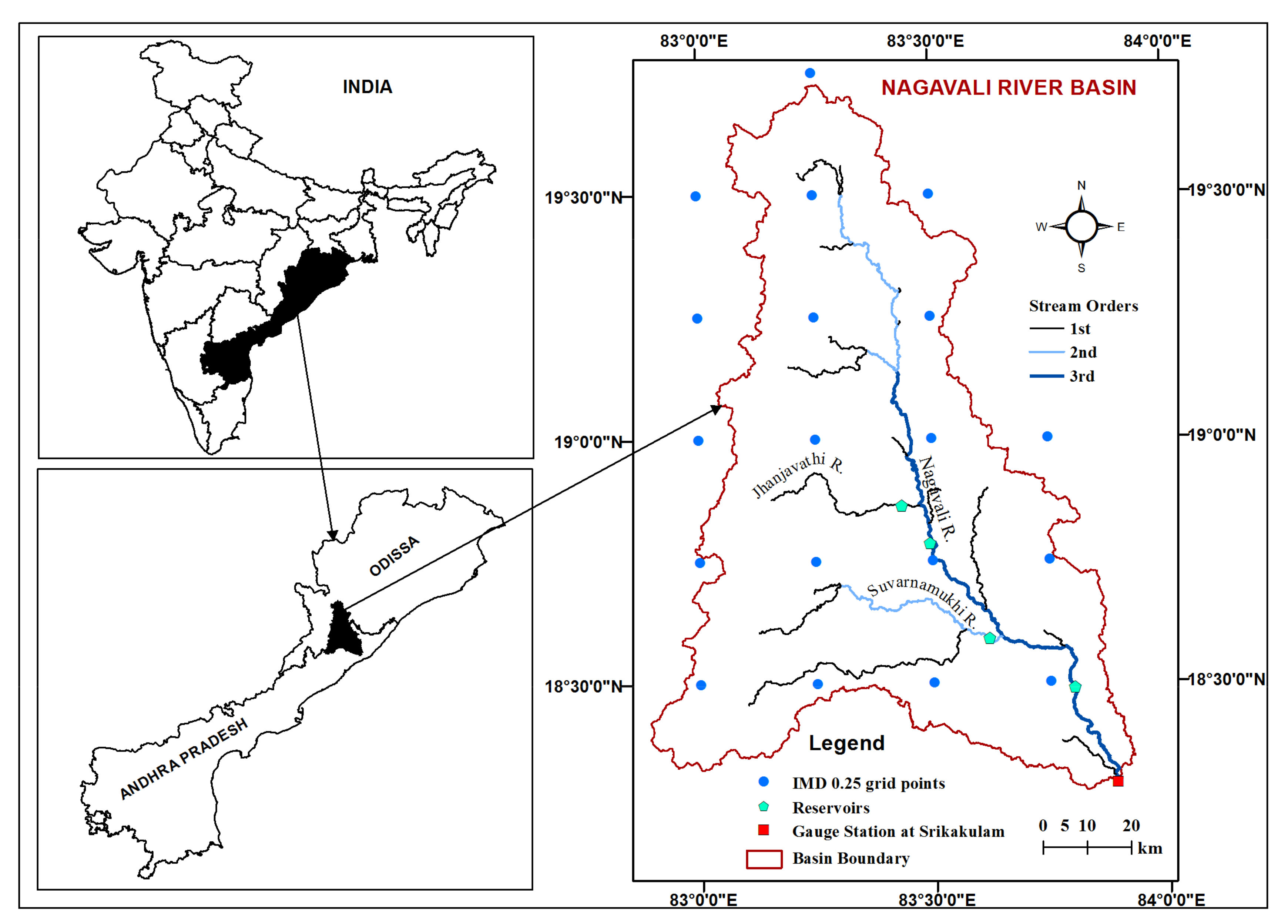
2.1. Study Area

We selected the Nagavali River Basin (NRB) since the literature on semi-arid and semi-humid climatic regions is limited. NRB lies between the Godavari and Mahanadi river basins in the eastern part of India, with a catchment area of about 9510 km² (Figure 1). The river begins from the Eastern Ghats at an elevation of 1600 m. It traverses about 160 km through Odisha and enters Andhra Pradesh near Kuneru village of Vizianagaram district at an elevation of about 152 m [55]. The extent of the basin is 18°17′ to 19°44′ north latitudes and 82°53′ to 83°54′ east longitudes. The stream length ranges around 255 km, out of which the main 62% lies in Odisha and the rest in Andhra Pradesh.

In this study, we considered the catchment area of 9056 km² up to the gauging and discharge measurement station at Srikakulam. NRB gets typical yearly precipitation of around 1140 mm, and the annual average temperature of the river basin is 28.2 °C in post-monsoon and 34.2 °C in pre-monsoon.

2.2. Datasets

Four precipitation products from different sources and of different resolutions that are the most frequently used in the hydrological application are used. This include gridded IMD (0.25° × 0.25°), TRMM 3B42 (0.25° × 0.25°), bias-corrected TRMM (0.25° × 0.25°) and reanalysis NCEP-CFSR (0.31° × 0.31°). All the datasets are selected for the common observation period from 1998–2012.

Table 1. Detailed information and sources of different rainfall datasets used in this study. IMD—Indian Meteorological Department; TRMM—Tropical Rainfall Measurement Mission; NCEP-CFSR National Center for Environmental Prediction Climate Forecast System Reanalysis.

Name and Type	Spatial Resolution/Coverage	Temporal Resolution/Period	Remarks, References and Data Sources
IMD (gridded rainfall dataset)	0.25°/Pan India	Daily/1901–2013	The gridded data were generated from the observed data of 6995 gauging stations across India using spatial interpolation for the period 1901–2013 [14] Details about these data can be obtained from http://imd.gov.in (homepage/rainfall information).
TRMM 3B42V7 (satellite product)	0.25°/Global (50 N-S)	Daily/1998–2014	Joint mission between the National Aeronautics and Space Administration (NASA) and the Japan Aerospace Exploration Agency (JAXA) to monitor tropical precipitation [6] one type of the TRMM multi-satellite precipitation analysis (TMPA) products) https://giovanni.gsfc.nasa.gov
Bias-corrected TRMM (satellite product)	0.25°/Global (50 N-S)	Daily/1998–2014)	The bias of TRMM rainfall was corrected by applying monthly multiplicative correction coefficients (MCC) of IMD rainfall [56] $MC{C}_{daily}=IM{D}_{total}/TRM{M}_{total}$ https://giovanni.gsfc.nasa.gov
CFSR (reanalysis dataset)	0.31°/Global (50 N-S)	Daily/1979–2014	Global, high resolution, coupled atmosphere–ocean–land surface-sea ice system started in 1979 by the National Centers for Environmental Prediction [22] https://globalweather.tamu.edu/

and Supplementary Information Section S1 present detailed information about the precipitation data.

2.3. Verification Strategy

Various statistical metrics used to evaluate the satellite precipitation products with reference to gauge-based IMD gridded data both qualitatively and quantitatively. IMD dataset is a popular validated dataset used in several other works [57,58,59,60,61]. Pai et al. [14] and Yeggina et al. [62] evaluated the performance of the IMD gridded dataset against the gauge rainfall estimates and showed that the IMD gridded dataset could be used as a reliable alternative for gauge rainfall. Various qualitative methods were used to measure the correspondence between estimates by precipitation product and IMD data. Here, we use the false alarm ratio (FAR), probability of detection (POD) and critical success index (CSI)—to evaluate the TRMM, bias-corrected TRMM and CFSR data with the reference rainfall data (IMD). Detailed information on these statistical metrics is presented in

Table 2. Definition of statistical metrics used to evaluate the TRMM, bias-corrected TRMM and CFSR data with the reference rainfall data (IMD). These statistical measures were computed by comparing rainfall and non-rainfall events for satellite (TRMM and CFSR) and reference (IMD) rainfall data. In general, when the values of probability of detection (POD) < 0.65, FAR > 0.35 and CSI < 0.45, it is assumed that the product performance is low in terms of detecting rainfall. The calculation of these three metrics is explained in [64].

S. No	Statistical Metrics	Equation	Description
1	Probability of detection (POD)	POD = H/(H + M)	It represents the detected rainfall events correctly by satellite out of rainfall events by reference data. Its ranges from 0 to 1 (1 is the best value)
2	False alarm ratio (FAR)	FAR = F/(F + H)	It represents the false, detected as rainfall event by satellite when reference data showed no rainfall. Its ranges from 0 to 1 (0 is the best value)
3	Critical success index (CSI)	CSI = H/(H + M + F)	It is more accurate when correct negative values are not considered. Its ranges from 0 to 1 (1 is the perfect value)

and Supplementary Information Section S2. Instead of point-to-point analysis, we analyzed the spatial average rainfall over the entire catchment considering the size and homogeneity of the catchment [63]. Based on the average rainfall for a given day, these statistical measures were computed by comparing rainfall and non-rainfall events for satellite (TRMM and CFSR) and reference (IMD) rainfall data.

For the verification of the discharge simulation from the hydrological model, we adopted the popular performance evaluation measures such as Nash–Sutcliffe coefficient (NS) [65], percentage of bias (PBIAS) and the coefficient of determination (R2) in this study.

$$NS=1-\left\{\frac{{{\displaystyle \sum }}_{i=1}^n{\left(Y_i^{obs}-Y_i^{sim}\right)}^2}{{{\displaystyle \sum }}_{i=1}^n{\left(Y_i^{obs}-\overline{Y}\right)}^2}\right\}$$

(1)

$$PBIAS=\left\{\frac{{{\displaystyle \sum }}_{i=1}^n\left(Y_i^{obs}-Y_i^{sim}\right)\times 100}{{{\displaystyle \sum }}_{i=1}^n\left(Y_i^{obs}\right)}\right\}$$

(2)

$$\mathrm{Correlation}\mathrm{coefficient}=\frac{{{\displaystyle \sum }}_{i-1}^n(Y_i^{obs}-{\overline{Y}}^{obs})\left(Y_i^{sim}-{\overline{Y}}^{sim}\right),}{\sqrt{{{\displaystyle \sum }}_{i-1}^n(Y_i^{obs}-{\overline{Y}}^{obs}}{)}^2\sqrt{\sqrt{{{\displaystyle \sum }}_{i-1}^n(Y_i^{sim}-{\overline{Y}}^{sim}}{)}^2}}$$

(3)

where $Y_i^{sim}$ and $Y_i^{obs}$ are the ith time step simulated and observed values, respectively. $\overline{Y}$ is the mean of ‘n’ observed values.

The values of NS ranges from −∞ to 1, with NS = 1 indicating the best model. PBIAS (Equation (2)) measures the average tendency of the simulated data (Gupta et al. [66], and the optimal value of PBIAS is zero. If PBIAS is a positive value, the model is underestimating the streamflow, and if PBIAS is negative, the model overestimates the streamflow. The model is unsatisfactory if NSE ≤ 0.5, satisfactory performance (0.5 < NS ≤ 0.65), good performance (0.65 < NS ≤ 0.75), very good performance (0.75 < NS ≤ 1.00) and PBIAS >± 25% for the streamflow [67]. The R2 pattern similarity between observed and simulated data and its value ranges between 0 and 1. Higher the value of R2, the higher the similarity.

2.4. Hydrological Model

The precipitation products mentioned above were used to drive a semi-distributed Soil and Water Assessment Tool (SWAT) model. Here, we briefly describe the SWAT model and its governing equations, procedures to set up the model, and finally, the way to calibrate and evaluate the model.

SWAT is a comprehensive, physically based, continuous in time, semi-distributed hydrological model [68,69]. It was developed by the Agriculture Research Service of the United States Department of Agriculture and used widely to study large scale hydrological conditions in different regions [70,71,72,73]. It mimics various hydrological components of watersheds by solving process-based equations. The various processes in the SWAT model are simulated at daily time steps based on the water balance equation (Equation (1), [74])

$${SW}_t={SW}_O+ {\displaystyle \sum }_{i=1}^t(R_{day}-Q_{surf}-E_a-W_{seep}-Q_{gw})$$

(4)

where $S{W}_o$ and $S{W}_t$ represent initial and water content at any time ‘t’ days (in mm), respectively. $E_a,R_{day} and Q_{surf}$ represent the amount of evapotranspiration, precipitation and surface runoff (in mm) on any day. The amount of percolation and return flow on a day $i$ (in mm) is denoted by $W_{seep}\&Q_{gw},$ respectively. The Soil Conservation Service (SCS)-curve number (CN) method (Equations (5) and (6)) is used for estimating the surface runoff.

$$Q_{surf}=\frac{{\left(R_{day}-{\mathrm{I}}_{\mathrm{a}}\right)}^2}{\left(R_{day}-{\mathrm{I}}_{\mathrm{a}}+S\right)}$$

(5)

$$S=254\left(\frac{CN}{100}\right)-1$$

(6)

Q_surf and R_day represent the accumulated runoff or rainfall excess (in mm) and rainfall received on that particular day (in mm), respectively [74]. I_a denotes an initial loss that includes detention, interception and percolation before the runoff. The retention factor is denoted by $S$ marks retention parameter. The retention factor is subjected to spatial variation owing to land-use change, soil type, various management options, slope and temporal variation because of the changes in soil water.

The storage routing technique is used for calculating the percolation (Arnold et al. [75], assuming that the percolation occurs whenever water content exceeds the field capacity, and the layer below is unsaturated (Mosbahi et al. 2020 [76], Sridhar, 2013 [53]). In this study, the Penman–Monteith method is adopted for estimating potential evapotranspiration. Using DEM, SWAT divides the entire basin into different subbasins and subsequently into hydrological response units (HRUs) based on the unique land use, soil classification, slope and various management combinations.

Primary meteorological variables such as temperature, precipitation, solar radiation, relative humidity and wind speed are required in addition to land use, soil characteristics and land cover to set up a hydrological model using SWAT. A brief description of the input data and data sources are presented in

Table 3. Detailed information on primary meteorological variables required to set up a hydrological model using the soil water assessment tool (SWAT).

Data Type	Scale	Source
Digital elevation model (DEM)	30 m × 30 m	Shuttle radar topography mission (SRTM) of USGS (https://earthexplorer.usgs.gov/)
Land use/land cover (LULC)	500 m	GIAM-IWMI (http://www.iwmi.cgiar.org)
Soil	1:1,500,000	http://www.fao.org/soils-portal/soil-survey/soil-maps-and-databases/faounesco-soil-map-of-the-world/en/ Food and Agriculture Organization (FAO)
Rainfall, temperature	0.25° (~32 km)	http://imdpune.gov.in/Clim_Pred_LRF_New/Grided_Data_Download.html Indian Metrological Department (IMD), PUNE
Solar radiation, relative humidity, wind speed	0.31° (~38 km)	https://rda.ucar.edu/datasets/ds093.1/ Climate Forecast System Reanalysis (CFSR)
Hydrological data	Daily	https://indiawris.gov.in/wris, (Central Water Commission (CWC)_

. Moreover, the land use land cover and soil map of the study area are shown in Figure 2. The daily river discharge data were obtained from the water resources information system of India (Central Water Commission, [77] for the period from 1985–2012 at Srikakulam station, as shown in Table 3. The reservoir details, inflow and outflow data were obtained from the Andhra Pradesh Water Resources Department and were incorporated in the model for implementing regulations.

QSWAT interfaced with a quantum geographical information system (QGIS) was used for developing the model. Preliminary analysis was done to re-project all the information to a common projection and was resampled to 30 m spatial resolution. TauDEM tool in QSWAT was used for stream network generation and watershed delineation. The entire basin was divided into 43 sub-basins using a threshold of 150 km². A total of 200 HRUs were formed by fixing a threshold of 200 HRUs with distinct land use, soil and slope. Here, the analysis was carried out at the hydrologic response unit (HRU) level on a monthly time step. Further, SWAT calibration and uncertainty procedures (CUP) 2012 with sequential uncertainty fitting (SUFI-2) was used for auto-calibration, sensitivity analysis and validation purposes (for more detail, please refer to Setti et al. [55].

3. Model Development and Evaluation

For simulating streamflow from different precipitation inputs, two different scenarios were considered, which are as follows:

Scenario A: calibrating the model with IMD gridded data and rerunning the model with other considered precipitation products; and

Scenario B: calibrating the model with each of the rainfall products.

Scenario A would allow investigating the impact of differences in rainfall products on streamflow simulation accuracy, whereas Scenario B (with each of rainfall products) will help in investigating the impact of input rainfall data on calibrated parameters, sensitivity analysis and streamflow simulation accuracy and in verifying whether these rainfall products can be used as an alternative source of input rainfall data for model calibration.

For both the scenarios, the sensitive parameters selection, automatic calibration and validation were performed by SUFI-2 optimization algorithms in the SWAT-CUP tool package. Sensitive parameters were identified using Latin-Hypercube One-factor-At-a-Time method with 2000 simulations. This procedure tests the model sensitivity by modifying only one parameter at a time and keeping the rest unchanged. In total, 18 parameters were identified from past literature (Setti et al. [63], and sensitivity analysis was performed.

In this study, we considered the first two years, i.e., 1998–2000, as the warm-up period to reduce the effect of initial conditions. The monthly simulated streamflow of the Nagavali River Basin was calibrated over a time period of 2001–2008 and then validated in the period of 2009–2012 with observation streamflow at Srikakulam station (as shown in Figure 1) using SWAT. For each iteration, 2000 simulations were run for the calibration period. Following each iteration, parameter ranges were modified (nearest to fitted value) with reference to the values suggested by the program and also by their reasonable physical limitations. Interested readers refer [78,79] for more details about the protocol to calibrate the SWAT model.

4. Results and Discussion

We present the results in three categories, first comparing satellite data and reanalysis data with ground-based IMD data, second, evaluating hydrological model based on the precipitation products for two different scenarios, and finally, comparison of the annual water balance components.

4.1. Comparison of Satellite Data and Reanalysis Data with Ground-Based IMD Data

First, we computed statistical parameters such as minimum rainfall, maximum rainfall, standard deviation, average and skewness coefficient of all precipitation products (

Table 4. Statistical measures of four considered rainfall data sets estimated using only rainy days (rainfall magnitude ≥2.5 mm/day) for the period from 1998–2013. TRMM—Tropical Rainfall Measurement Mission; IMD—Indian Meteorological Department; NCEP-CFSR National Center for Environmental Prediction Climate Forecast System Reanalysis.

Statistical Measures	IMD	TRMM	Bias Corrected TRMM	CFSR
Minimum rainfall (mm)	2.5	2.5	2.5	2.5
Maximum rainfall (mm)	140.2	157.7	119.4	176.4
Mean rainfall (mm)	11.9	13.3	11.9	12.6
Standard deviation(mm)	12.7	13.7	11.9	13.1
Skewness	3.8	3.4	3.2	4.3

) only for rainy days (rainfall magnitude ≥2.5 mm/day).

We observed that the maximum precipitation values were slightly overestimated by TRMM and CFSR datasets in comparison with the IMD product. Similarly, the CFSR is more positively skewed than the IMD, showing the general tendency for overestimation. The empirical cumulative density function (CDF) of the daily precipitation distribution during 1998–2012 was computed for the four datasets (Figure 3). There is a slight difference in the CDF obtained for IMD, TRMM and CFSR data at low values of rainfall. However, the deviation is significant in the precipitation range from 30 to 60 mm/day for TRMM and CFSR data. The CDF of the bias-corrected TRMM is closely matching with that of IMD.

IMD dataset for the time period from 1998–2013 revealed a total of 1591 rainy days and 4252 non-rainy days. On the other hand, the total rainy days estimated by the TRMM, bias-corrected TRMM and CFSR are 978, 932 and 1161, respectively (

Table 5. Contingency table for category estimation of rainy days and non-rainy days between observed rainfall and satellite rainfall (TRMM and CFSR) with 2.5 mm/day threshold value during the period of 1998–2013.

Event	IMD	Observed Event	TRMM	Bias Corrected TRMM	CFSR
Rainy days	1591	Hit (H)	978	932	1161
		Miss (M)	613	659	430
Non-rainy days	4253	False alarm (F)	718	658	712
		Correct negative	3535	3595	3541

).

Using the threshold of 2.5 mm/day, the values of POD, FAR and CSI were estimated. The value of POD was found to be around 0.61, 0.69 and 0.73 (

Table 6. Statistical metrics are calculated for daily data of Nagavali River Basin based on an average of 19 rainfall grids for the time series of 1998–2013.

Statistical Metrics		TRMM	Bias Corrected TRMM	CFSR
Probability of detection	POD	0.61	0.69	0.73
False alarm ratio	FAR	0.42	0.39	0.38
Critical success index	CSI	0.42	0.45	0.50

) for TRMM, bias-corrected TRMM and CFSR, respectively, indicating the CFSR product is close to the IMD dataset in terms of hits. Similarly, in terms of FAR and CSI, the CFSR data seems to perform better than the TRMM-based datasets. For example, the CFSR data have the lowest value of FAR (0.38) and the highest value of CSI (0.50). These analyses showed that the CFSR product has better performance than the other products like TRMM and bias-corrected TRMM. However, it to be noted that this analysis does not consider the quantity of the rainfall; instead, it only finds hits and misses into consideration.

In order to compare the data products based on the rainfall amount, we choose the rainfall intensity classification of the World Meteorological Organization (WMO) standard Geneva, Switzerland, 2012 [80] (1) rain < 2.5 mm (no/tiny rain), (2) 2.5 mm ≤ rain < 5 mm (low moderate rain), (3) 5 mm ≤ rain < 10 mm (high moderate rain), (4) 10 mm ≤ rain < 20 mm (low heavy rain),(5) 20 mm ≤ rain < 50 mm (high heavy rain),and (6) rain ≥ 50 mm (violent rain). The four considered precipitation datasets display a similar probability of occurrence of dry days (rain < 2.5 mm/d), which are 49%, 44%, 44% and 37% for IMD, TRMM, bias-corrected TRMM and CFSR, respectively. However, within the wet days, the probability of occurrence of high, moderate rain (low heavy rain) was found to be 30% (22%), 26% (25%), 28% (24%) and 31% (27%) for IMD, TRMM, bias-corrected TRMM and CFSR, respectively. It is observed that the CFSR data have more probability of occurrence in the low heavy rain range than what is observed in IMD data.

To evaluate the overall pattern and rainfall quantity, rainfall datasets on three different time scales—daily, monthly and annual—were considered. On a daily scale, the linear Pearson correlation between the IMD and other data sets such as TRMM, bias-corrected TRMM and CFSR datasets was found to be 0.44, 0.83 and 0.82, respectively. The daily and average monthly time series of the rainfall events of four datasets are shown in Figure 4a,b. It is evident that there is a significant difference between precipitation products. The monthly variation of the precipitation values shows there is no systematic over or under prediction by CFSR or TRMM data. For example, during the 2003 monsoon, CFSR and TRMM overestimated the rainfall, whereas during the years 2004 and 2005, the rainfall was underestimated. On the annual time scale (Figure 4c), different products show that there is a strong similarity in terms of rainfall totals for the most part of the study period. However, in the latter part of the study period (2009–2013), TRMM and CFSR data overestimate the rainfall compared to the IMD-based values. The standard deviation of the four precipitation datasets computed at the annual time scale over the 16 years considered is 270 mm, 222 mm, 193 mm and 415 mm for the IMD, TRMM, bias-corrected TRMM and CFSR, respectively and the results of two-sample Kolmogorov–Smirnov (Setti et al. [63] tests at the 5% significance level indicate that the four precipitation datasets have different statistical distributions in the study area.

4.2. Hydrological Model-Based Evaluation of the Precipitation Products

As mentioned, two different scenarios were considered-calibrating the SWAT model with IMD gridded data and rerunning the model with other considered precipitation products.

4.2.1. Scenario A: SWAT Model Calibrated with IMD Data

This scenario attempts to unravel the effects of the precipitation products on streamflow simulation, specifically when the precipitation products driving the model is calibrated with IMD data.

4.2.2. Calibration of the SWAT Model with IMD Data

Initially, model calibration was done using the IMD rainfall data as input to the model after finding the sensitive parameters (using the method mentioned in Section 3). The calibration was done using the SWAT-CUP with the objective function of maximizing the NS between the observed and simulated flows. The performance statistics of the models’ simulation showed that the calibration is good with reference to NS and correlation coefficient on the order of 0.85 and 0.79 and 0.91 and 0.88, respectively, during the calibration and validation periods.

In the second step, the other precipitation products are used for driving the calibrated model. Figure 5 shows the streamflow simulation results from each of the precipitation products, and the corresponding performance statistics are shown in

Table 7. Comparison of the satellite streamflow simulation performance statistics for Scenario A (model calibrated with IMD data).

Statistical Metrics	Performance of Different Datasets under Scenario A
	IMD	TRMM	Bias Corrected TRMM	CFSR
R2	0.87	0.60	0.68	0.54
NS	0.85	0.55	0.62	0.52
PBIAS	−5.5	−15.3	−7.4	−16.2
P-factor	0.83	0.65	0.8	0.65
r-factor	0.67	0.48	0.63	0.91

. It is observed that even though the TRMM dataset-based model is performing satisfactorily in driving the model, according to Moriasi et al. [67]. However, streamflow estimates show systematic overestimation with PBIAS = −15.3%. Interestingly, the systematic difference has significantly reduced in the bias-corrected TRMM-based model with PBIAS = −7.4%. The streamflow simulation using the CFSR data seems to be overestimated with PBIAS = −16.2%. However, it is to be noted that in the case of the CFSR, the streamflow overestimations are not systematic; rather, the pattern streamflow closely follows the precipitation pattern. There is considerable streamflow overestimation in the year 2003, during which the rainfall estimates were higher than the IMD data. On the other hand, the streamflow simulation was underestimated during the years 2000, 2004 and 2005, where the rainfall estimates from CFSR were lower than IMD. Thus, there is no systematic under or overestimation in the streamflow simulation.

These aforementioned results demonstrated that the bias-corrected TRMM data are a potential alternative to IMD data.

4.2.3. Scenario B: SWAT Model Calibrated Individually with Precipitation Products

This scenario evaluates the applicability of the precipitation products for calibrating the model and investigates the differences in model calibration, sensitive parameters and the ability to simulate streamflow accurately.

4.2.4. Sensitive Parameters

To evaluate the difference introduced at the stage of sensitivity analysis by using different precipitation products, we compared the ranking of the sensitive parameters obtained. Out of several parameters, we selected 18 commonly used parameters (

Table 8. Description of parameters and their range values used for sensitivity analysis.

S. No	Parameter	Description	Min	Max
1	CN2.mgt *	SCS runoff curve number for moisture condition II, which controls the surface runoff	−0.1	0.1
2	ALPHA_BF.gw	Baseflow alpha factor for groundwater flow response to changes in recharge	0	1
3	GW_DELAY.gw	Groundwater delay represents the time taken by water move from the bottom soil layer to the upper shallow aquifer (days)	30	450
4	GWQMN.gw	Threshold depth of water in the shallow aquifer required for return flow to occur. If it is decreased, baseflow will be decreased (in mm)	0	5000
5	GW_REVAP.gw	Groundwater “revap” coefficient (Water movement from shallow aquifer to vegetation roots). If it is close to zero, the movement of water is restricted; if it approaches 1, the rate of water approaches the rate of evapotranspiration	0.02	0.2
6	RCHRG_DP.gw	Deep aquifer percolation fraction from the root zone which recharges in a deep aquifer	0	1
7	REVAPMN.gw	Threshold depth of water in the shallow aquifer for “revap” to occur (mm). Controls the water movement from a shallow aquifer to a deep aquifer	0	1000
8	SLSUBBSN.hru	Average slope length	10	150
9	HRU_SLP.hru	Average slope steepness (m/m)	0	1
10	OV_N.hru	Manning’s “n” value for overland flow	0.01	30
11	LAT_TTIME.hru	Lateral flow travel time (days)	0	180
12	ESCO.hru	Soil evaporation compensation factor (represents the process of evapotranspiration from soil moisture to atmosphere, if the ESCO is reduced, the evaporation is increased)	0	1
13	EPCO.hru	Plant uptake compensation factor (The amount of water uptake by a plant for transpiration, If EPCO value is 1, the model allows more of the water uptake demand)	0	1
14	SURLAG.bsn	Surface runoff lags time (days). It controls the fraction of water to allow to the reach on the day	0.05	24
15	SOL_AWC().sol	Available water capacity of the soil layer	0	1
16	SOL_K().sol	Saturated hydraulic conductivity (mm/h). This relates to soil water flow rate to the hydraulic gradient.	0	2000
17	CH_K2.rte	Effective hydraulic conductivity in main channel alluvium (mm/h). If streams have continuous groundwater contribution, the effective conductivity will be zero.	0.1	500
18	ALPHA_BNK.rte	Baseflow alpha factor for bank storage (Contributes flow to the reach within the subbasin)	0	1

* Indicates that the CN2 values are reported as percentages of variation of the original value.

) for streamflow simulation using four precipitation products.

To identify the sensitivity parameters of each precipitation dataset, the model was run with 2000 simulations of eighteen selected parameters. Interestingly, the most sensitive parameters obtained for the four datasets were significantly different (

Table 9. Sensitivity parameter ranking for each dataset with default parameter values using sequential uncertainty fitting (SUFI)-2 algorithm. Interestingly, the most sensitive parameters obtained for the four datasets were significantly different except for the deep percolation factor and curve number (CN2) that comes out to be significant for all products. The second most significant factor was soil evaporation compensation factor (ESCO) using IMD and TRMM, whereas it was baseflow alpha factor (ALPHA_BF) and threshold depth of water in the shallow aquifer (GWQMN) using bias-corrected TRMM and CFSR data.

S. No	Parameter	IMD	TRMM	Bias Corrected TRMM	CFSR
1	r__CN2.mgt	6	1	2	1
2	v__ALPHA_BF.gw	18	18	17	14
3	v__GW_DELAY.gw	12	13	15	10
4	v__GWQMN.gw	3	6	8	3
5	v__GW_REVAP.gw	5	8	14	5
6	v__RCHRG_DP.gw	1	2	3	2
7	v__REVAPMN.gw	13	10	10	15
8	v__SLSUBBSN.hru	7	4	4	6
9	v__HRU_SLP.hru	8	5	6	7
10	v__OV_N.hru	16	11	12	11
11	v__LAT_TTIME.hru	17	7	7	9
12	v__ESCO.hru	2	3	1	4
13	v__EPCO.hru	11	12	11	17
14	v__SURLAG.bsn	15	16	18	18
15	r__SOL_AWC().sol	9	9	5	8
16	r__SOL_K().sol	14	14	9	13
17	v__CH_K2.rte	10	17	16	12
18	v__ALPHA_BNK.rte	4	15	13	16

) except for the deep percolation factor and curve number (CN2) that comes out to be significant for all products. The second most significant factor was ESCO using IMD and TRMM, whereas it was ALPHA_BF and GWQMN using bias-corrected TRMM and CFSR data. The most sensitive parameters from all the data sets include RCHRG_DP, ESCO and GWQMN, which show that the crucial processes governing the hydrology of the system are evapotranspiration and groundwater recharge, which is in line with the general understanding of the dominant processes in forest and agricultural catchment.

4.2.5. Model Calibration

Here, out of the eighteen parameters, the ten most sensitive parameters for each dataset were further considered for calibration of the corresponding models.

The individual models were developed based on four different data sets and were calibrated at a monthly scale using the SUFI-2 algorithm. The results from the model calibration are enumerated for all the models in

Table 10. Comparison of NS and R² values during the calibration (2000–2008) and validation (2009–2012) periods obtained when models were recalibrated with individual precipitation product as input.

Statistical Results during the Calibration and Validation Period
Statistical Metrics	Calibration				Validation
	IMD	TRMM	TRMM-Bias	CFSR	IMD	TRMM	Bias Corrected TRMM	CFSR
R2	0.87	0.76	0.78	0.77	0.82	0.77	0.74	0.74
NS	0.85	0.71	0.74	0.76	0.79	0.72	0.72	0.73
PBIAS	−5.5	−13.4	−7.2	−14.3	−6.2	−15.2	−8.1	−17.2
P-factor	0.83	0.68	0.72	0.64	0.85	0.67	0.69	0.61
r-factor	0.67	0.46	0.59	0.40	0.79	0.44	0.61	0.41

. Following the model performance classification of Moriasi et al. [67], the model based on IMD precipitation data performs well with NS (R²) values on the range 0.85(0.87) and 0.79(0.82) during the calibration and validation period, respectively. On the other hand, the CFSR data-based model performance is satisfactory with the NS values 0.76 and 0.73 during calibration and validation, respectively. The models based on TRMM and bias-corrected TRMM dataset produced better results with NS equal to 0.71 and 0.74, respectively, as shown in Table 10. A similar pattern was observed in the PBIAS values during the calibration and validation period.

Figure 6 shows the streamflow simulation results during calibration and validation. Based on the simulation results obtained during calibration and validation, it can be seen that the IMD data produces the best results in comparison with the other datasets. However, closer simulation was obtained using the TRMM bias-corrected dataset. It is also to be noted that the bias-corrected TRMM datasets are yielding better results when compared to the TRMM data. Further, the results based on CFSR are also satisfactory when compared to its performance in Scenario A. However, there is an overestimation of streamflow for most of the simulations except for the years 2000, 2004 and 2005. This implies that the recalibration of the model with the individual dataset has increased the model performance to a greater extent. A similar observation was also reported by Tuo et al. [2] and Zhang et al. [41].

Besides the evaluation of the results from the best simulation from each precipitation data set, as explained above, we also investigated the ensemble of all available simulations. We calculated the distribution of the NSC values obtained for the total of 2000 simulations. Figure 7 shows the empirical CDF of the NSC values obtained from the four models. All four models reached a satisfactory level of performance. However, interesting results were obtained using the bias-corrected TRMM data set, where most of the simulations (around 80% of the model simulations) were above NSC = 0.5, while IMD, TRMM, CFSR data sets had a lower fraction on the order of 70%, 20% and 65%, respectively. IMD data-based model displays a larger fraction (50%) of model simulations having NSC > 0.65, which represents excellent model performance. On comparing the bias-corrected TRMM dataset and TRMM-based models, there is a significant improvement in the bias-corrected TRMM-based results. This analysis indicates the uncertainty in terms of model performance when using different precipitation data sets.

4.2.6. Parameter Uncertainty

The parameter uncertainty when using different precipitation data sets was estimated by investigating the variations in the best-fit parameters, and the range of parameters obtained during the calibration.

Table 11. Values for best-fit parameters obtained using the four different datasets. Among the important parameters, ESCO, an important parameter related to soil evaporation, have different ranges for the different datasets. The range of the parameters for ESCO obtained using IMD is different from the ones obtained from other precipitation data sets.

S. No	Parameter	IMD	TRMM	Bias Corrected TRMM	CFSR
1	v__ESCO.hru	0.11	0.56	0.06	0.67
2	v__SLSUBBSN.hru	42.59	145.7	36.7	145.6
3	v__HRU_SLP.hru	0.28	0.06	1.0	0.11
4	r__SOL_AWC().sol	−0.03	0.037	0.054	0.03
5	r__CH_K2.rte	367.1	X	X	X
6	r__CN2.mgt	−0.152	−0.09	-0.15	−0.19
7	V__ALPHA_BNK.rte	0.33	X	X	X
8	V__RCHRG_DP.gw	0.073	0.047	0.06	0.011
9	V__GW_REVAP.gw	0.13	0.079	X	0.115
10	V__GWQMN.gw	4577	3196	3234	3942
11	V__OV_N.hru	X	13.47	X	21.1
12	V__LAT_TTIME.hru	X	85	47	28.8
13	V__GW_DELAY.gw	X	X	X	72

and Figure 8 show the values and range of the best-fit parameters of the calibrated parameters of nine global sensitive hydrological parameters, respectively. Among the critical parameters shown in Figure 8, ESCO, an important parameter related to soil evaporation, have different ranges for the different datasets. It is also to be noted that the range of the parameters for ESCO obtained using IMD is different from the ones obtained from other precipitation data sets. TRMM and CFSR dataset-based models have a high ESCO value >0.5 when compared to IMD, and TRMM bias-corrected-based models indicate lower evapotranspiration compared to other datasets, which are also reflected in overestimation of streamflow.

Deep aquifer percolation fraction (RCHRG_DP) (the most dominant parameter in four precipitation datasets) displays variation in both best values and the ranges considering all the precipitation inputs. This indicates that the IMD-based model allows more water for deep percolation when compared to the CFSR-driven model. Similarly, the best parameter ranges for GWQMN (a parameter controlling the depth of water in the shallow aquifer) were higher for the IMD-based model when compared to the other models, which indicates the model-based in TRMM and CFSR data resulted in less shallow aquifer storage.

Interestingly, there is no significant difference in the CN2 parameter, which reflects the surface runoff in terms of both the best parameter and the ranges. However, for other parameters, such as SOL _AWC, HRU_SLP, CH_K2, the ranges and the best fit values are different.

Overall, the analysis shows that different precipitation inputs affect both the best estimate of a parameter as well as its ranges. It is to be noted that the SWAT-CUP adjusts parameters in such a way that the observed streamflow values are matched. Even though the models capture the observed flow, the parameter values, and hence the distribution of water in the catchment, are entirely different. For example, the average water balances of the various components in the study area using different precipitation data set lead to different values of evapotranspiration, base flow, percolation, but more or less similar surface runoff values. It can be observed that the calibrated bias-corrected TRMM forced the model to have low ESCO when compared to the other models resulting in higher values of evapotranspiration.

4.2.7. Uncertainty in Streamflow Simulation

Even though the parameter uncertainties contribute to uncertainty in all outputs, variables were obtained from the model. In this section, we limit our discussion only to the uncertainty in the streamflow, as shown in Figure 9. We evaluated the uncertainty using the p-factor, and R-factor obtained during the calibration. The p-factor represents the fraction of observed streamflow falling within the 95PPU band and varies from 0 to 1, where p = 1 indicates that 100% of the observed flow falls within the 95% confidence band (i.e., a perfect model simulation considering the uncertainty). The R-factor is estimated as the ratio of the average width of the 95% confidence band and the standard deviation of the observed streamflow. A value of R < 1.5, again depending on the situation, would be desirable for this index. According to Abbaspour et al. [81], R-value less than 1.5 would be desirable for satisfactory model simulation.

In this study, the percentage of observed data bracketed by 95PPU uncertainty for IMD, TRMM, bias-corrected TRMM and CFSR is 83%, 68%, 72% and 64%, respectively during the calibration and 85%, 67%, 69% and 61%, respectively during the validation period as shown in Figure 9 and Table 10. However, comparing the r-factors (which measures the width of the 95PPU), it can be observed that the CFSR and bias-corrected TRMM-based models have low values indicating the higher levels of uncertainty. Further, the observed peak values do not fall within the 95PPU obtained from these data sets. Thus, it is clear from these results different precipitation inputs generate discrete prediction uncertainties for estimation of streamflow.

4.3. Comparison of the Annual Water Balance

Figure 10 represents the annual average of the water balance components based on the different rainfall inputs. For comparison, the observed streamflow and evapotraspiration (ET) are provided from the literature. Figure 10a presents the results of the models calibrated with IMD data (Scenario A), and Figure 10b shows the results of the model obtained when calibrated with individual data rainfall type.

4.3.1. Precipitation

The catchment averaged rainfall estimates from the TRMM and CFSR indicate that these data sets have a general tendency for overestimating the rainfall when compared to the IMD datasets. This is consistent with the results reported in [41].

4.3.2. Streamflow

On comparing the observed and the simulated streamflow volume, we noted that the model based on IMD data produced annual streamflow accurately; nevertheless, the performance of other data sets depends on how the model was calibrated.

When the model was calibrated with IMD data (Scenario A), the CFSR-based model overestimated the average annual streamflow. In particular, it can be seen from Figure 5 that the non-monsoon streamflow was higher. However, TRMM and bias-corrected TRMM models result in slight over and underestimation, respectively. The results closely follow the pattern in the rainfall estimates showing that rainfall is the primary driving factor in streamflow simulation. Under Scenario B, all the models show comparatively better ability in capturing the streamflow volume; however, bias-corrected TRMM showed the ability to reproduce the streamflow accurately. Moreover, significant improvement in the CFSR data-based model was reported.

4.3.3. Evapotranspiration

The IMD-based model simulation of ET (641.5 mm) was well within the range of 600–700 mm in the study area [53]. Under Scenario A, TRMM, CFSR, and bias-corrected TRMM resulted in an overestimation of the ET, but the amount of overestimation is different. Even though TRMM and CFSR have similar precipitation amounts, but the distribution of the water balance components is different. This difference may be attributed to the difference in the rainfall pattern and intensity, as discussed in Section 4.1. On calibrating the model with the satellite data sets (the objective function used here is the performance of streamflow volume), TRMM and bias-corrected TRMM significantly overestimated the ET, whereas the CFSR data resulted in lesser value and close to IMD-based model estimation. Overall, we notice a considerable increase in both ET and streamflow estimates for all the data sets due to the overestimation of the rainfall.

It was observed that the precipitation dataset is primary data in driving hydrological model and also the main source of uncertainty as different precipitation dataset leads to different best parameter ranges. Further, uncertainty in the input precipitation propagates to the uncertainty to the model estimates of the water balance components and, therefore, on the water resources management and policy decisions made based on the model results.

5. Conclusions

We compared four different precipitation datasets of different categories, source and resolution, namely IMD, TRMM, bias-corrected TRMM and CFSR using a hydrological model. We investigated the impact of precipitation products on hydrological model calibration, model predictions for a forest-dominated river basin in India. The following are salient features obtained from the study.

All the considered precipitation products showed a good correlation with each other as well as the IMD gridded data on a daily scale. The CC of CFSR and bias-corrected TRMM with the IMD data were approximately 0.8. However, a quantitative comparison of the precipitation showed that CFSR and TRMM data have a slight tendency to overestimate precipitation. We also observed that bias-corrected TRMM data are comparable with the IMD data. The deviation is significant in the precipitation range from 30 mm/day to 60 mm/day.

We created two scenarios were for evaluating the precipitation using the SWAT model. In Scenario A, the model was calibrated using IMD precipitation data as input, and later this model was run with other data sets. In Scenario B, individual models were developed with each of the rainfall products as input. From these scenarios, we observed that the performance of streamflow modeling increased when the model was calibrated individually for each of the rainfall products.

The results from Scenario B showed that the different precipitation datasets resulted in multiple sets of sensitive parameters, parameter ranges and water balance components. The IMD data-based model yielded the best results in terms of streamflow simulation. The model based on the bias-corrected TRMM dataset produced closer results and thus can be used as an alternate for gauge precipitation. In summary, the choice of precipitation products has a vital role in model performance, prediction uncertainties and parameter uncertainties in streamflow simulations. Water balance estimation based on different precipitation datasets can lead to different conclusions, and therefore uncertainty generated by the use of different precipitation inputs must be taken into consideration.

References

1. Tuo, Y.; Marcolini, G.; Disse, M.; Chiogna, G. A multi-objective approach to improve SWAT model calibration in alpine catchments. J. Hydrol. 2018, 559, 347–360. [Google Scholar] [CrossRef]
2. Agarwal, A.; Marwan, N.; Maheswaran, R.; Ozturk, U.; Kurths, J.; Merz, B. Optimal Design of Hydrometric Station Networks Based on Complex Network Analysis. J. Hydrol. Earth Syst. Sci. 2020, 24, 2235–2251. [Google Scholar] [CrossRef]
3. Dile, Y.T.; Srinivasan, R. Evaluation of CFSR climate data for hydrologic prediction in data-scarce watersheds: An application in the Blue Nile River Basin. J. Am. Water Resour. Assoc. (JAWRA) 2014, 50, 1226–1241. [Google Scholar] [CrossRef]
4. Rienecker, M.M.; Suarez, M.J.; Gelaro, R.; Todling, R.; Bacmeister, J.; Liu, E.; Woollen, J. MERRA: NASA’s Modern-Era Retrospective Analysis for Research and Applications. J. Clim. 2011, 24, 3624–3648. [Google Scholar] [CrossRef]
5. Rodell, M.; Houser, P.R.; Jambor, U.E.A.; Gottschalck, J.; Mitchell, K.; Meng, C.J.; Arsenault, K.; Cosgrove, B.; Radakovich, J.; Bosilovich, M.; et al. The global land data assimilation system. Bull. Am. Meteorol. Soc. 2004, 85, 381–394. [Google Scholar] [CrossRef] [Green Version]
6. Huffman, G.J.; Adler, R.F.; Bolvin, D.T.T.; Gu, G.; Nelkin, E.J.; Bowman, K.P.; Hong, Y.; Stocker, E.F.; Wolff, D.B. The TRMM Multisatellite Precipitation Analysis (TMPA): Quasi-global, multiyear, combined-sensor precipitation estimates at fine scales. J. Hydrometeorol. 2007, 8, 38–55. [Google Scholar] [CrossRef]
7. Hong, Y.; Hsu, K.L.; Sorooshian, S.; Gao, X.G. Precipitation estimation from remotely sensed imagery using an artificial neural network cloud classification system. J. Appl. Meteorol. 2004, 43, 1834–1852. [Google Scholar] [CrossRef] [Green Version]
8. Joyce, R.J.; Janowiak, J.E.; Arkin, P.A.; Xie, P. CMORPH: A method that produces global precipitation estimates from passive microwave and infrared data at high spatial and temporal resolution. J. Hydrometeorol. 2004, 5, 487–503. [Google Scholar] [CrossRef]
9. Funk, C.; Peterson, P.; Peterson, S.; Shukla, S.; Davenport, F.; Michaelsen, J.; Knapp, K.R.; Landsfeld, M.; Husak, G.; Harrison, L.; et al. A High-Resolution 1983–2016 T max Climate Data Record Based on Infrared Temperatures and Stations by the Climate Hazard Center. J. Clim. 2019, 32, 5639–5658. [Google Scholar] [CrossRef]
10. Hou, A.; Jackson, G.S.; Kummerow, C.; Shepherd, J.M. Global precipitation measurement. In Precipitation: Advances in Measurement, Estimation, and Prediction; Michaelides, S., Ed.; Springer: Berlin, Germany, 2008; pp. 131–170. [Google Scholar]
11. Hou, A.Y.; Kakar, R.K.; Neeck, S.; Azarbarzin, A.A.; Kummerow, C.D.; Kojima, M.; Oki, R.; Nakamura, K.; Iguchi, T. The global precipitation measurement mission. Bull. Am. Meteorol. Soc. 2014, 95, 701–722. [Google Scholar] [CrossRef]
12. Hamada, A.; Arakawa, O.; Yatagai, A. An automated quality control method for daily rain-gauge data. Glob. Environ. Res. 2011, 15, 165–172. [Google Scholar]
13. Yatagai, A.; Kamiguchi, K.; Arakawa, O.; Hamada, A.; Yasutomi, N.; Kitoh, A. APHRODITE: Constructing a long-term daily gridded precipitation dataset for Asia based on a dense network of rain gauges. Bull. Am. Meteorol. Soc. 2012, 93, 1401–1415. [Google Scholar] [CrossRef]
14. Pai, D.S.; Sridhar, L.; Rajeevan, M.; Sreejith, O.P.; Satbhai, N.S.; Mukhopadhyay, B. (1901–2010) daily gridded rainfall data set over India and its comparison with existing data sets over the region. Mausam 2014, 1, 1–18. [Google Scholar]
15. Li, D.; Christakos, G.; Ding, X.; Wu, J. Adequacy of TRMM satellite rainfall data in driving the SWAT modeling of Tiaoxi catchment (Taihu lake basin, China). J. Hydrol. 2018, 556, 1139–1152. [Google Scholar] [CrossRef]
16. Wang, A.; Zeng, X. Evaluation of multireanalysis products with in situ observations over the Tibetan Plateau. J. Geophys. Res. Atmos. 2012, 117, 1–12. [Google Scholar] [CrossRef]
17. Stisen, S.; Sandholt, I. Evaluation of remote-sensing-based rainfall products through predictive capability in hydrological runoff modelling. Hydrol. Process. 2010, 24, 879–891. [Google Scholar] [CrossRef]
18. Skinner, C.J.; Coulthard, T.J.; Parsons, D.R.; Ramirez, J.A.; Mullen, L.; Manson, S. Simulating tidal and storm surge hydraulics with a simple 2D inertia based model, in the Humber Estuary, U.K. Estuar. Coast. Shelf Sci. 2015, 155, 126–136. [Google Scholar] [CrossRef]
19. Qi, J.; Zhang, X.; McCarty, G.W.; Sadeghi, A.M.; Cosh, M.H.; Zeng, X.; Gao, F.; Daughtry, C.S.; Huang, C.; Lang, M.W.; et al. Assessing the performance of a physically-based soil moisture module integrated within the Soil and Water Assessment Tool. J. Environ. Model. Softw. 2018, 109, 329–341. [Google Scholar] [CrossRef]
20. Yu, Y.; Wang, J.; Cheng, F.; Deng, H.; Chen, S. Drought monitoring in Yunnan Province based on a TRMM precipitation product. J. Nat. Hazards 2020, 104, 2369–2387. [Google Scholar] [CrossRef]
21. Tuo, Y.; Duan, Z.; Disse, M.; Chiogna, G. Evaluation of precipitation input for SWAT modeling in Alpine catchment: A case study in the Adige river basin (Italy). Sci. Total Environ. 2016, 573, 66–82. [Google Scholar] [CrossRef] [Green Version]
22. Fuka, D.R.; Walter, M.T.; MacAlister, C.; Degaetano, A.T.; Steenhuis, T.S.; Easton, Z.M. Using the climate forecast system reanalysis as weather input data for watershed models. Hydrol. Process. 2013, 28, 5613–5623. [Google Scholar] [CrossRef]
23. Wang, J.; Hong, Y.; Li, L.; Gourley, J.J.; Khan, S.I.; Yilmaz, K.K.; Limaye, A.S. The coupled routing and excess storage (CREST) distributed hydrological model. Hydrol. Sci. J. 2011, 56, 84–98. [Google Scholar] [CrossRef]
24. Roth, V.; Lemann, T. Comparing CFSR and conventional weather data for discharge and soil loss modelling with SWAT in small catchments in the Ethiopian highlands. Hydrol. Earth Syst. Sci. 2016, 20, 921–934. [Google Scholar] [CrossRef] [Green Version]
25. Tolera, M.B.; Chung, I.M.; Chang, S.W. Evaluation of the climate forecast system reanalysis weather data for watershed modeling in Upper Awash basin, Ethiopia. Water 2018, 10, 725. [Google Scholar] [CrossRef] [Green Version]
26. Zhu, D.; Ren, Q. Hydrological evaluation of hourly merged satellite—Station precipitation product in the mountainous basin of China using a distributed hydrological model. Meteorol. Appl. 2020, 27, e1909. [Google Scholar] [CrossRef]
27. Ma, M.; Wang, H.; Jia, P.; Tang, G.; Wang, D.; Ma, Z.; Yan, H. Application of the GPM-IMERG Products in Flash Flood Warning: A Case Study in Yunnan, China. Remote Sens. 2020, 12, 1954. [Google Scholar] [CrossRef]
28. Yeditha, P.K.; Venkatesh, K.; Maheswaran, R.; Ankit, A. Forecasting of extreme flood events using different satellite precipitation products and wavelet-based machine learning methods. Chaos Interdiscip. J. Nonlinear Sci. 2020, 30, 063115. [Google Scholar] [CrossRef]
29. Bitew, M.M.; Gebremichael, M. Evaluation of satellite rainfall products through hydrologic simulation in a fully distributed hydrologic model. Water Resour. Res. 2011, 47, 1–11. [Google Scholar] [CrossRef]
30. Vu, M.T.T.; Raghavan, S.V.; Liong, S.Y.Y. SWAT use of gridded observations for simulating runoff—A Vietnam river basin study. Hydrol. Earth Syst. Sci. 2012, 16, 2801–2811. [Google Scholar] [CrossRef] [Green Version]
31. Tang, G.; Zeng, Z.; Long, D.; Guo, X.; Yong, B.; Zhang, W.; Hong, Y. Statistical and hydrological comparisons between TRMM and GPM Level-3 products over a midlatitude Basin: Is day-1 IMERG a good successor for TMPA 3B42V7? J. Hydrometeorol. 2016, 17, 121–137. [Google Scholar] [CrossRef]
32. Zhu, H.; Li, Y.; Huang, Y.; Li, Y.; Hou, C.; Shi, X. Evaluation and hydrological application of satellite-based precipitation datasets in driving hydrological models over the Huifa river basin in Northeast China. J. Atmos. Res. 2018, 207, 28–41. [Google Scholar] [CrossRef]
33. Huang, S.; Chang, J.; Leng, G.; Huang, Q. Integrated index for drought assessment based on variable fuzzy set theory: A case study in the Yellow River basin, China. J. Hydrol. 2015, 527, 608–618. [Google Scholar] [CrossRef]
34. Sun, R.; Yuan, H.; Liu, X.; Jiang, X. Evaluation of the latest satellite-gauge precipitation products and their hydrologic applications over the Huaihe River basin. J. Hydrol. 2016, 536, 302–319. [Google Scholar] [CrossRef]
35. Wang, Z.; Zhong, R.; Lai, C.; Chen, J. Evaluation of the GPM IMERG satellite-based precipitation products and the hydrological utility. Atmos. Res. 2017, 196, 151–163. [Google Scholar] [CrossRef]
36. Yilmaz, K.K.; Hogue, T.S.; Hsu, K.L.; Sorooshian, S.; Gupta, H.V.; Wagener, T. Intercomparison of rain gauge, radar, and satellite-based precipitation estimates with emphasis on hydrologic forecasting. J. Hydrometeorol. 2005, 6, 497–517. [Google Scholar] [CrossRef]
37. Su, F.; Hong, Y.; Lettenmaier, D.P. Evaluation of TRMM multisatellite precipitation analysis (TMPA) and its utility in hydrologic prediction in the La Plata Basin. J. Hydrometeorol. 2008, 9, 622–640. [Google Scholar] [CrossRef] [Green Version]
38. Gao, Z.; Long, D.; Tang, G.; Zeng, C.; Huang, J.; Hong, Y. Assessing the potential of satellite-based precipitation estimates for flood frequency analysis in ungauged or poorly gauged tributaries of China’s Yangtze River basin. J. Hydrol. 2017, 550, 478–496. [Google Scholar] [CrossRef]
39. Maggioni, V.; Massari, C. On the performance of satellite precipitation products in riverine flood modeling: A review. J. Hydrol. 2018, 558, 214–224. [Google Scholar] [CrossRef]
40. Jiang, L.; Bauer-Gottwein, P. How do GPM IMERG precipitation estimates perform as hydrological model forcing? Evaluation for 300 catchments across Mainland China. J. Hydrol. 2019, 572, 486–500. [Google Scholar] [CrossRef]
41. Zhang, Z.; Tian, J.; Huang, Y.; Chen, X.; Chen, S.; Duan, Z. Hydrologic evaluation of TRMM and GPM IMERG satellite-based precipitation in a humid basin of China. Remote Sens. 2019, 11, 431. [Google Scholar] [CrossRef] [Green Version]
42. Jiang, D.; Wang, K. The role of satellite-based remote sensing in improving simulated streamflow: A review. Water 2019, 11, 1615. [Google Scholar] [CrossRef] [Green Version]
43. Yuan, F.; Zhang, L.; Soe, K.M.W.; Ren, L.; Zhao, C.; Zhu, Y.; Jiang, S.; Liu, Y. Applications of TRMM- and GPM-era multiple- satellite precipitation products for flood simulations at sub-daily scales in a sparsely gauged watershed in Myanmar. Remote Sens. 2019, 11, 140. [Google Scholar] [CrossRef] [Green Version]
44. Grassotti, C.; Hoffman, R.N.; Vivoni, E.R.; Entekhabi, D. Multiple-timescale intercomparison of two radar products and rain gauge observations over the Arkansas—Red River basin. J. Weather Forecast. 2003, 18, 1207–1229. [Google Scholar] [CrossRef] [Green Version]
45. Yang, F.; Zhang, G.L.; Yang, J.L.; Li, D.C.; Zhao, Y.G.; Liu, F.; Yang, R.M.; Yang, F. Organic matter controls of soil water retention in an alpine grassland and its significance for hydrological processes. J. Hydrol. 2014, 519, 3010–3027. [Google Scholar] [CrossRef]
46. Le, M.H.; Lakshmi, V.; Bolten, J.; Du Bui, D. Adequacy of Satellite-derived Precipitation Estimate for Hydrological modeling in Vietnam Basins. J. Hydrol. 2020, 586, 124820. [Google Scholar] [CrossRef]
47. Guo, D.; Wang, H.; Zhang, X.; Liu, G. Evaluation and analysis of grid precipitation fusion products in Jinsha river basin based on China meteorological assimilation datasets for the SWAT model. Water 2019, 11, 253. [Google Scholar] [CrossRef] [Green Version]
48. Jiang, L.; Madsen, H.; Bauer-Gottwein, P. Simultaneous calibration of multiple hydrodynamic model parameters using satellite altimetry observations of water surface elevation in the Songhua River. Remote Sens. Environ. 2019, 225, 229–247. [Google Scholar] [CrossRef]
49. Harris, A.; Rahman, S.; Hossain, F.; Yarborough, L.; Bagtzoglou, A.C.; Easson, G. Satellite-based flood modeling using TRMM-based rainfall products. J. Sens. 2007, 7, 3416–3427. [Google Scholar] [CrossRef] [Green Version]
50. Su, J.; Lü, H.; Zhu, Y.; Cui, Y.; Wang, X. Evaluating the hydrological utility of latest IMERG products over the Upper Huaihe River Basin, China. J. Atmos. Res. 2019, 225, 17–29. [Google Scholar] [CrossRef]
51. Jiang, Q.; Li, W.; Wen, J.; Qiu, C.; Sun, W.; Fang, Q.; Xu, M.; Tan, J. Accuracy evaluation of two high-resolution satellite-based rainfall products: TRMM 3B42V7 and CMORPH in Shanghai. Water 2018, 10, 40. [Google Scholar] [CrossRef] [Green Version]
52. Shukla, R.; Agarwal, A.; Gornott, C.; Sachdeva, K.; Joshi, P.K. Farmer typology to understand differentiated climate change adaptation in Himalaya. Sci. Rep. 2019, 9, 20375. [Google Scholar] [CrossRef] [PubMed] [Green Version]
53. Abbaspour, K.C.; Yang, J.; Maximov, I.; Siber, R.; Bogner, K.; Mieleitner, J.; Zobrist, J.; Srinivasan, R. Modelling hydrology and water quality in the pre-alpine/alpine Thur watershed using SWAT. J. Hydrol. 2007, 333, 413–430. [Google Scholar] [CrossRef]
54. Sridhar, V. Tracking the influence of irrigation on land surface fluxes and boundary layer climatology. J. Contemp. Water Res. Educ. 2013, 152, 79–93. [Google Scholar] [CrossRef]
55. Setti, S.; Rathinasamy, M.; Chandramouli, S. Assessment of water balance for a forest dominated coastal river basin in India using a semi distributed hydrological model. Model. Earth Syst. Environ. 2017, 4, 127–140. [Google Scholar] [CrossRef]
56. Haerter, J.O.; Hagemann, S.; Moseley, C.; Piani, C. Climate model bias correction and the role of timescales. Hydrol. Earth Syst. Sci. 2011, 15, 1065–1079. [Google Scholar] [CrossRef] [Green Version]
57. Sridhar, V.; Wedin, D.A. Hydrological behavior of Grasslands of the Sandhills: Water and Energy Balance Assessment from Measurements, Treatments and Modeling. Ecohydrology 2009, 2, 195–212. [Google Scholar] [CrossRef]
58. Guntu, R.K.; Rathinasamy, M.; Agarwal, A.; Sivakumar, B. Spatiotemporal variability of Indian rainfall using multiscale entropy. J. Hydrol. 2020, 587, 124916. [Google Scholar] [CrossRef]
59. Guntu, R.K.; Maheswaran, R.; Agarwal, A.; Singh, V.P. Accounting for temporal variability for improved precipitation regionalization based on self-organizing map coupled with information theory. J. Hydrol. 2020, 590, 125236. [Google Scholar] [CrossRef]
60. Agarwal, A. Unraveling Spatio-Temporal Climatic Patterns via Multi-Scale Complex Networks. PhD Thesis, Universität Potsdam, Potsdam, Germany, 2019. [Google Scholar]
61. Kurths, J.; Agarwal, A.; Marwan, N.; Rathinasamy, M.; Caesar, L.; Krishnan, R.; Merz, B. Unraveling the spatial diversity of Indian precipitation teleconnections via nonlinear multi-scale approach. Nonlinear Process. Geophys. 2019, 26, 251–266. [Google Scholar] [CrossRef] [Green Version]
62. Yeggina, S.; Teegavarapu, R.S.; Muddu, S. Evaluation and bias corrections of gridded precipitation data for hydrologic modelling support in Kabini River basin, India. Theor. Appl. Climatol. 2020, 140, 1495–1513. [Google Scholar] [CrossRef]
63. Setti, S.; Maheswaran, R.; Radha, D.; Sridhar, V.; Asce, M.; Barik, K.K.; Narasimham, M.L. Attribution of Hydrologic Changes in a Tropical River Basin to Rainfall Variability and Land-Use Change: Case Study from India. J. Hydrol. Eng. 2020, 25, 1–15. [Google Scholar] [CrossRef]
64. AghaKouchak, A.; Mehran, A. Extended contingency table: Performance metrics for satellite observations and climate model simulations. Water Resour. Res. 2013, 49, 7144–7149. [Google Scholar] [CrossRef] [Green Version]
65. Nash, J.E.; Sutcliffe, J.V. River flow forecasting through conceptual models part I- A discussion of principles. J. Hydrol. 1970, 10, 282–290. [Google Scholar] [CrossRef]
66. Gupta, H.V.; Sorooshian, S.; Yapo, P.O. Status of automatic Calibration for hydrologic models: Comparison with multilevel expert calibration. J. Hydrol. Eng. 1999, 4, 135–143. [Google Scholar] [CrossRef]
67. Moriasi, D.N.; Arnold, J.G.; Van Liew, M.W.; Bingner, R.L.; Harmel, R.D.; Veith, T.L. Model evaluation guidelines for systematic quantification of accuracy in watershed simulations. J. Trans. ASABE 2007, 50, 885–900. [Google Scholar] [CrossRef]
68. Arnold, J.G.; Moriasi, D.N.; Gassman, P.W.; Abbaspour, K.C.; White, M.J.; Griensven, V.; Liew, V. DigitalCommons@University of Nebraska-Lincoln SWAT: Model use, calibration, and validation. Biol. Syst. Eng. Pap. Publ. 2012. [Google Scholar] [CrossRef]
69. Arnold, J.G.; Srinivasan, R.; Muttiah, R.S.; Williams, J.R. Large area hydrologic modeling and assessment part I: Model development. J. Am. Water Resour. Assoc. 1998, 34, 73–89. [Google Scholar] [CrossRef]
70. Kang, H.; Sridhar, V. Combined statistical and spatially distributed hydrological model for evaluating future drought indices in Virginia. J. Hydrol. Reg. Stud. 2017, 12, 253–272. [Google Scholar] [CrossRef]
71. Kang, H.; Sridhar, V. Improved drought prediction using near real-time climate forecasts and simulated hydrologic conditions. Sustainability 2018, 10, 1799. [Google Scholar] [CrossRef] [Green Version]
72. Sehgal, V.; Sridhar, V.; Juran, L.; Ogejo, J. Integrating Climate Forecasts with the Soil and Water Assessment Tool (SWAT) for High-Resolution Hydrologic Simulation and Forecasts in the Southeastern USS. Sustainability 2018, 10, 3079. [Google Scholar] [CrossRef] [Green Version]
73. Sridhar, V.; Kang, H.; Ali, S.A. Human-induced alterations to land use and climate and their responses on hydrology and water management in the Mekong River basin. Water 2019, 11, 1307. [Google Scholar] [CrossRef] [Green Version]
74. Neitsch, S.L.; Arnold, J.G.; Kiniry, J.R.; Srinivasan, R.; Williams, J.R. Soil & Water Assessment Tool: Input/Output Documentation; Version 2012. TR-439; Texas Water Resources Institute: College Station, TX, USA, 2012. [Google Scholar]
75. Arnold, J.G.; Williams, J.R.; Maidment, D.R. Continuous-time water and sediment-routing model for large basins. J. Hydraul. Eng. 1995, 121, 171–183. [Google Scholar] [CrossRef]
76. Mosbahi, M.; Benabdallah, S. Assessment of land management practices on soil erosion using SWAT model in a Tunisian semi-arid catchment. J. Soils Sediments 2020, 1129–1139. [Google Scholar] [CrossRef]
77. CWC (Central Water Commission). Stream Flow Discharge Data for the Period 1985–2012. 2018. Available online: http://cwc.gov.in/water-resources-information-system-wris (accessed on 22 March 2018).
78. Abbaspour, K.C. SWAT-CUP: SWAT Calibration and Uncertainty Programs—A User Manual. 2015. Available online: http://swat.tamu.edu/software/swatcup/ (accessed on 10 August 2016).
79. Abbaspour, K.C.; Rouholahnejad, E.; Vaghefi, S.; Srinivasan, R.; Yang, H.; Kløve, B. A continental-scale hydrology and water quality model for Europe: Calibration and uncertainty of a high-resolution large-scale SWAT model. J. Hydrol. 2015, 524, 733–752. [Google Scholar] [CrossRef] [Green Version]
80. World Meteorological Organization. Observation of present and past weather state of the ground. In Guide to Meteorological Instruments and Methods of Observation; Chapter 14; WMO: Geneva, Switzerland, 2012; pp. 14–19. [Google Scholar]
81. Abbaspour, K.C.; Johnson, C.A.; van Genuchten, M.T. Estimating uncertain flow and transport parameters using a sequential uncertainty fitting procedure. Vadose Zone J. 2004, 3, 1340–1352. [Google Scholar] [CrossRef]
Figure 1. Index map showing the geographical location of Nagavali River Basin (NRB) along with the stream network, gauge location in red and precipitation grid points in blue. Total 19 grid points of the Indian Meteorological Department (IMD) were located within the NRB river basin.
Atmosphere 11 01252 g001
Figure 2. Land use land cover classification (a) and soil map (b) with subbasins for Nagavali River Basin (NRB). QSWAT interfaced with a quantum geographical information system (QGIS) was used for developing the hydrological model.
Atmosphere 11 01252 g002
Figure 3. Cumulative probability of four daily precipitation datasets (IMD, TRMM, bias-corrected TRMM, CFSR) for NRB. Distribution of all precipitation values (a); distribution of precipitation below 30 mm (b); distribution of precipitation values between 30 mm to 60 mm (c).
Atmosphere 11 01252 g003
Figure 4. Comparison between observed rainfall product (IMD), satellite precipitation products (TRMM, bias-corrected) and reanalysis data (CFSR) at daily (a), monthly (b) and (c) annual scale.
Atmosphere 11 01252 g004
Figure 5. Comparison of streamflow simulation obtained from model calibrated with IMD data when driven using different precipitation datasets during the period (2000–2008).
Atmosphere 11 01252 g005
Figure 6. Simulated and observed hydrograph of the best simulation during the calibration (2000–2008) and validation periods (2009–2012) of four dataset products when the models were individually calibrated with the corresponding precipitation datasets.
Atmosphere 11 01252 g006
Figure 7. Distribution of Nash simulation values during calibration obtained using different precipitation datasets for the Nagavali River Basin.
Atmosphere 11 01252 g007
Figure 8. Calibrated parameter ranges (y-axis) of global sensitive hydrological parameters for the four precipitation datasets within the initial parameter range.
Atmosphere 11 01252 g008
Figure 9. 95PPU plots along with the observed and simulated flows using best parameter values for the four datasets during the calibration period (2000–2008) at the monthly time scale.
Atmosphere 11 01252 g009
Figure 10. The annual average of hydrologic components such as precipitation, streamflow and evapotranspiration obtained using different rainfall inputs for a model calibrated with (a) IMD data and (b) individual rainfall data.
Atmosphere 11 01252 g010