Article

Simulating Water and Salt Migration through Soils with a Clay Layer and Subsurface Pipe Drainage System at Different Depths Using the DRAINMOD-S Model

1
College of Water Conservancy and Civil Engineering, Inner Mongolia Agricultural University, Hohhot 010018, China
2
High Efficiency Water-Saving Technology and Equipment and Soil and Water Environment Effect in Engineering Research Center of Inner Mongolia Autonomous Region, Hohhot 010018, China
3
School of Materials Science and Engineering, Beihang University, Beijing 100191, China
*
Authors to whom correspondence should be addressed.
Agronomy 2024, 14(1), 17; https://doi.org/10.3390/agronomy14010017
Submission received: 31 October 2023 / Revised: 19 December 2023 / Accepted: 19 December 2023 / Published: 20 December 2023

Abstract

:
Soil salinization affects more than 25% of land globally. Subsurface pipe drainage is known for its effectiveness in improving saline–alkali land. The red clay layer (RCL) hinders soil improvement in the Hetao Irrigation District of Inner Mongolia, China. The soil water and salt migration rules at different buried depths and RCL were studied based on the field subsurface pipe drainage test and simulation using the DRAINMOD-S model (Version 6.1). The following implications can be drawn from the results: (1) Although the RCL affected the accuracy of the model, the calibrated statistical results met the application requirements, and the DRAINMOD-S model can be used to analyze subsurface pipe drainage under different distribution conditions of the RCL. (2) The RCL can reduce the drainage efficiency of the subsurface pipe, specifically when the distribution is shallow. (3) The soil desalting rate increased with an increase in the buried depth of the subsurface pipe. The desalination effect of shallow soil was better than that of deep soil. The RCL reduced the drainage and salt removal efficiency of the subsurface pipe. Burying the subsurface pipe as far above the RCL as possible should be considered. Thus, it is feasible to apply the DRAINMOD-S model to relevant studies.

1. Introduction

Soil salinization has been widely researched, particularly as it has contributed to the global food security crisis in the 21st century [1]. The Hetao Irrigation District of Inner Mongolia, China, is a crucial production base for commodity grains and oil. As the largest single-system artesian irrigation basin in Asia, it is under serious threat from soil salinization [2,3,4]; in addition, 63.8% of the soil in the irrigated area is salinized, resulting in soil nutrient loss, crop reduction, farmland wastage, and other issues that seriously restrict the potential for sustainable development in this area [5,6]. Several scholars have attempted to improve saline soils, including the addition of organic and inorganic substances such as fly ash, water-retaining agents, soybean straw, and other single-type amendments, mineralizing soil ions, and laying effective irrigation and drainage facilities [7,8,9,10]. Among these approaches, subsurface pipe drainage engineering is popular owing to its advantages in improving land-use efficiency, strong applicability, and remarkable improvement. The successful global application of subsurface drainage pipes has created a novel approach for saline–alkali land improvement strategies [11,12].
The different layout parameters of subsurface pipes and migration laws of soil water, salt, and nutrients are usually the focus of subsurface pipe drainage engineering research [13,14,15]. Some scholars have found that the salt discharge of subsurface pipes is positively correlated with burial depth, whereas it is negatively and linearly correlated with spacing [16]. Increasing the drainage distance of subsurface pipes or decreasing the drainage depth can reduce NO 3 -N loss [17,18]. The appropriate arrangement of subsurface pipes differs with different research objectives and field soil conditions (such as groundwater depth and soil texture). Canola cultivation occurs in consolidated, subsurface-drained paddy fields under winter rainfed conditions. To reduce the loss of NO 3 -N and water and the impact of drainage on the environment, Hashemi et al. suggested that the subsurface pipe should be buried at a depth of 0.4 m and a spacing of 50 m [19]. However, in studies on saline–alkali land improvement in arid and semi-arid areas, Qian et al. found that the buried depth of subsurface pipes is often greater than 1 m and that subsurface pipes can achieve effective desalting effects [16]. Based on traditional subsurface pipe drainage, scholars have developed a compound improvement method that can prevent excessive drainage and reduce nutrient loss by controlling drainage more effectively [20,21]. Drainage circulation facilities can then be integrated with the control drainage system to alleviate drought, reduce agricultural nonpoint source pollution, and increase crop yield [22,23]. With gradual improvements in drainage engineering, research has advanced. Owing to the large number of research projects and the high cost of the drainage engineering layout, it is difficult to conduct large-scale research involving field experiments. However, the application of a numerical model to simulate subsurface pipe drainage can solve this problem.
DRAINMOD is a hydrological drainage model that is based on subsurface drainage. Compared with other models used in drainage research, DRAINMOD has several advantages, including fewer data requirements, simpler operation, high simulation accuracy, and strong applicability [24]. A study by Pourgholam-Amiji et al. demonstrated the feasibility of the DRAINMOD-S model in predicting and modeling soil salinity trends and revealed that the model is more advantageous when the simulated soil salt content is high [24]. Ghane and Askar used DRAINMOD to investigate and forecast shallow drainage systems in the United States, and Moursi et al. used DRAINMOD to predict the water efficiency of a drainage system [25,26]. The DRAINMOD model can be used to optimize the design of the system, improve the performance of subsurface pipes to improve saline-alkali soil, and reduce construction costs. Awad et al. used an artificial neural network system to improve DRAINMOD [27]. The improved model enhanced the precision of the groundwater table and surface water storage simulations. Lisenbee et al. successfully applied the DRAINMOD model to a bioretention system [28]. The rapid development and application of the DRAINMOD model demonstrate its substantial potential. The feasibility of applying the model in a complex drainage environment is demonstrated, which provides a prerequisite for successful application in this study.
As a common soil stratification in China [29], the red clay layer (RCL) is widely distributed in the Hetao Irrigation District. Its high water retention and low permeability make saline–alkali improvements more challenging. However, there are relatively few studies on whether the existence of the RCL will reduce the efficiency of subsurface pipe in saline-alkali soil improvement, and it is necessary to accurately clarify the relevant laws in the future. Therefore, to solve this problem, this study used the DRAINMOD-S model combined with field experiments to explore the soil water and salt transport rules under different distribution positions of the subsurface pipe and RCL and to clarify the effect of soil improvement on the existence of the RCL. This study provides reliable data to support the improvement of saline-alkali land in the future.

2. Materials and Methods

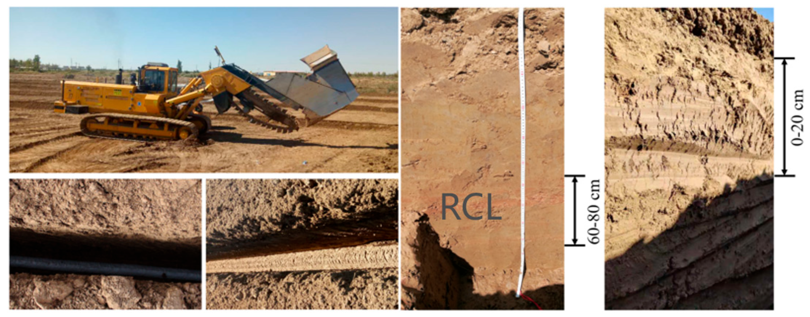
2.1. Study Area and Experimental Design

The Hetao Irrigation District, which is the largest gravity irrigation area in Asia, is the largest production base of commodity grain, oil, agricultural, and livestock products in China. The study area was located in the comprehensive improvement test base of subsurface pipe drainage (40°45′28″ N, 108°38′16″ E) in the Wulat irrigation area in the lower reaches of the district. The area has a temperate, arid, and semi-arid continental monsoon climate. Average temperature, precipitation, evaporation, and duration of sunshine when measured over several years were 6–8 °C, 196–215 mm, 2172.5 mm, and 3230.9 h, respectively. The soil salt content in the test area was very high (15.93 g/kg), with mostly salinized and severely salinized soils.
The subsurface pipe installation began in September 2018. After the soil settled and the underground pipe drainage system stabilized, a subsurface pipe drainage test was conducted from May 2019 to December 2020. A Netherlands INTER-DRAIN pipe-laying machine was used for subsurface pipe laying. The slope of the subsurface pipe was 1‰, the pipe diameter was 8 cm, and the length was 200 m. The distribution of the RCL in the soil profile was recorded and classified during the excavation of the subsurface pipe (Figure 1). In the whole soil profile, the color of the RCL was red. In terms of particle size classification, the particle size of the RCL was relatively small, the soil was finer silty soil, and its saturated hydraulic conductivity was considerably lower than that of other soil layers. In this experiment, four RCL distribution conditions were selected when the spacing of the subsurface pipe was 1000 cm and the burial depths were 80, 100, or 120 cm. Four RCL distribution conditions (no RCL, 0–20 cm or 60–80 cm with RCL, 0–20 cm, and 60–80 cm with RCL) and 12 plots were studied. Limited by the distribution of the RCL, 12 test plots were distributed at different locations on the test site. During the two-year experiment, irrigation was performed seven times (specifically, flood irrigation). The irrigations were 3000 m3/ha on 15 May 2019; 1500 m3/ha on 26 June 2019; 1500 m3/ha on 17 July 2019; 3000 m3/ha on 25 October 2019; 3500 m3/ha on 3 May 2020; 2500 m3/ha on 28 June 2020; and 3500 m3/ha on 19 October 2020.

2.2. Sampling, Measurement, and Calculation

The particle size distribution of the soil was measured using a laser particle size analyzer (HELOS-OASZS, SYMPATEC, Clausthal-Zellerfeld, Germany) [4]. The undisturbed soil collected from the test-site profile was returned to the laboratory for bulk density measurements. After grinding and sifting the dry soil samples, 10 g samples were collected, 50 mL of distilled water was added, and the mixture was oscillated and stirred for 5 min at room temperature (23–28 °C). After standing for 24 h, the conductivity (EC) of the soil-water solution of the extract was measured using a conductivity tylometer (DDS-307 A, REX, Shanghai, China) [5]. Equation (1) was used to calculate the total soluble salt (TDS) content [30]. The soil parameters of each soil layer are listed in Table 1. To obtain accurate data on irrigation water quantity, an inlet gate was installed at the irrigation outlet, and a meter ruler and a current meter (LS300-A, Nanjing Shengrong Instrument, Nanjing, China) were used for measurements.
TDS:
TDS   = 3.7657 EC 1 : 5   0.2405
where TDS is the soil salt content (g/kg) and EC1:5 is the EC of the soil extract solution prepared by mixing the soil with water at a soil:water ratio of 1:5 (mS/cm).
Three subsurface pipes with the same buried depth and spacing were arranged in each test plot, and only the soil near the middle subsurface pipe was selected as the research target to avoid interference from water and salt transport in adjacent plots. During the subsurface pipe drainage stage, the daily subsurface pipe drainage volume and drainage EC values were collected and monitored at the subsurface pipe drainage outlet in the middle of each test plot. Soil sampling points and groundwater level observation wells were arranged on one side of the middle subsurface pipe in each test plot. Soil samples were collected 24 h before irrigation and 24 h after drainage. Samples were collected every 20 cm, and the water content and EC of the soil samples were measured. The soil desalting rate was used to determine the desalting effect of irrigation in each experimental plot. The calculation method for the soil desalting rate is shown in Equation (2).
Soil desalting rate:
N = S 1   S 2 S 1 × 100 %
where N is the soil desalting rate (%), S1 is the initial soil salinity before irrigation (g/kg), and S2 is the soil salinity after irrigation (g/kg).

2.3. DRAINMOD-S Model

2.3.1. Model Description, Input Data, and Application

Compared with the DRAINMOD model [31], the DRAINMOD-S model (Version 6.1) added a salt module, which simulated the salt discharged from the subsurface pipe and the salt distribution in the soil profile. The water balance equation was used as the basis for the water simulation. The water balance calculation of the model was divided into surface and subsurface conditions (Equations (3) and (4)).
Δ W = P + I F RO
Δ V a = D + ET + VLS   F
where ΔW is the change in surface water storage (cm); P is the precipitation (cm); I is the irrigation quantity (cm); F is the infiltration amount (cm); RO is the surface runoff (cm); ΔVa is the change in water content of anhydrous pore space in the soil profile (cm); D is the subsurface displacement (cm); ET is the evapotranspiration (cm); and VLS is the vertical and lateral flow (cm). The Green–Ampt equation [32] was used to estimate the amount of infiltration. There was a 1 m high ridge around the test site. During the test period, all irrigation water was discharged through subsurface drainage, and no surface runoff was generated. The RO item was negligible. When there is water on the local surface, the Kirkham formula [33] is used to calculate the underground drainage. When the water level Is below the surface, the Hooghout steady flow formula [34] is used for calculation. Vertical and lateral seepage is estimated using a simple method based on Darcy’s law and the Dupuit–Forchheimer assumptions, but is negligible when the underlying permeability is poor.
The main input items of the model Ide meteorological, soil and crop data, and drainage system layout parameters. Meteorological data include precipitation, temperature, and sunshine radiation throughout the simulation cycle. Combined with the measured meteorological data, the reference daily evaporation was calculated using the Penman–Monteith formula [35] or Thornthwaite [36]. The irrigation water and irrigation time data are incorporated into the meteorological data module and input into the model. If the soil is layered, the required soil data should include the thickness of the soil layer, the water characteristic curve of each layer of soil, saturated hydraulic conductivity, and the initial salt content of the soil. Crop parameters include information such as the root depth of the crop, the date of planting and harvesting, and drought stress. However, the experimental plot has been abandoned on saline-alkali land for many years, and the degree of salinization is serious. Salt-tolerant plants, including weeds, cannot grow normally. Therefore, crops are not considered in this study, and information about crops and other aspects does not need to be entered. Drainage system parameters include drainage spacing, drainage depth, effective drainage radius, drainage coefficient, impermeable layer, and aquitard depth.
The water characteristic curve of the soil samples at the test site was obtained by laboratory detection, and parameters such as saturated water conductivity and initial soil salt content were input as data related to the model [18]. Meteorological data were obtained from a microweather station (HOBO-U30, Onset, Bourne, MA, USA) set up at the experimental site, and the main data included daily maximum and minimum temperatures, precipitation, wind speed, and radiation amount [18]. After inputting the meteorological data, the model calculates the potential evapotranspiration (PET) using the Penman–Monteith formula and determines the value of PET. When the soil moisture content is lower than the wilting point, the actual evapotranspiration is limited by the upward flux of soil moisture. When the moisture content of the soil at the root zone is above the wilting point, ET is set as the PET. The parameters of the field management system include the buried depth and spacing of the subsurface pipe, the initial depth of groundwater, the maximum storage depth of the surface, the effective drainage radius, the drainage coefficient, and the Kirkham depth flowing to the subsurface pipe. The parameter setting values are shown in Table 2.
Based on 12 field-test arrangements, the calibrated DRAINMOD-S model was used to simulate the buried pipe spacing of 10 m and buried depths of 40, 50, 60, 80, 100, and 120 cm. A total of 24 simulation test plots under four types of RCL distribution conditions (no RCL, 0–20 cm or 60–80 cm with RCL, 0–20 cm, and 60–80 cm with RCL) were used.

2.3.2. Calibration and Validation of the DRAINMOD-S Model

When calibrating the model, combined with previous studies [24], it was found that the transverse saturated hydraulic conductivity parameter is the most sensitive. Other sensitive parameters include impervious layer depth, maximum surface water storage depth, drainage coefficient, and initial groundwater level depth. The values of the parameters after verification are shown in Table 2. The DRAINMOD-S model is often calibrated using drainage volume, groundwater level, or soil salt content. In this study, according to the experimental design, the groundwater level and soil salt content data for the day within 24 h before and after each irrigation in 2019 were used for calibration, and the groundwater level and soil salt content data for the day within 24 h before and after each irrigation in 2020 were used for verification (Table 3 and Table 4). Multiple sets of statistical data were used to evaluate the model’s performance, including the deterministic coefficient (R2), mean absolute error (MAE), root mean square error (RMSE), and normalized root mean square error (NRMSE). Related research has shown that when R2 is greater than 0.5 and NRMSE is less than 30%, the model is reasonable and acceptable. The closer the MAE and RMSE were to 0, the higher the matching degree between the simulated and measured data [37,38]. These indices are calculated by Equations (5)–(8):
R 2 = ( i = 1 n ( O i O ¯ ) ( A i A ¯ ) ) 2 i = 1 n ( O i O ¯ ) 2 i = 1 n ( A i A ¯ ) 2
MAE = i = 1 n | A i O i | n
RMSE = 1 n i = 1 n ( A i O i ) 2
NRMSE = RMSE O ¯ × 100  
where Ai is the simulated value, A ¯ is the averaged simulated value, Oi is the observed value, O ¯ is the averaged observed value, and n is the sample size.

3. Results and Analysis

3.1. Model Evaluation

Table 3 shows the calibration and verification results of the groundwater level simulated by the model in the 12 experimental plots from 2019 to 2020. The R2 value is between 0.73 and 0.92, the MAE value is 5.06–19.12 cm, the RMSE is 5.83–20.15 cm, and the NRMSE is 7.36–27.08%. This shows that the simulation accuracy of the DRAINMOD-S model in hydrology meets the application requirements.
As shown in Table 4, the R2 value of the existing 12 experimental plots is between 0.60 and 0.90 in 2019–2020, the MAE value is 4.31–16.64 g/kg, the RMSE is 5.39–17.88 g/kg, and the NRMSE is 7.36–27.08%. The accuracy of the model simulation satisfied these requirements; therefore, it can be applied to simulate soil water and salt transport in arid regions containing RCL. By comparing the statistical results of each plot, we found that the overall simulation accuracy of the model decreased as the distribution range of the RCL increased in soils. The R2 value of the model under the condition of no RCL was 0.81–0.90, the R2 value of the model under one layer of the RCL was 0.70–0.88, and the R2 value under two layers of the RCL was 0.6–0.82. This phenomenon may be related to the model input parameters such as the soil water characteristic curve, soil saturated hydraulic conductivity, and initial soil salinity. DRAINMOD is a quasi-two-dimensional model, and, as a result, the soil properties of a profile are represented by a point of soil parameters. In the case of more complex soil properties, it is more difficult to use the average value of different soil layers to accurately represent the soil properties of each layer, resulting in a decrease in the accuracy of the simulation. By comparing the evaluation results of the plots with one layer of the RCL, it was found that the simulation accuracy of the plots with a 60–80 cm RCL was higher than that of the plots with a 0–20 cm RCL. The average R2 decreased from 0.86 to 0.79, and the average NRMSE increased from 16.75% to 18.54%, indicating that the distribution position of the RCL in the profile affected the fitting accuracy of the model. The closer the distribution position was to the surface, the lower the simulation accuracy. The average R2 value of each plot decreased from 0.82 (0.8 m) to 0.80 (1.2 m) with an increase in the buried depth of the pipe, and the buried depth of the pipe affected the accuracy of the simulation.
According to previous studies and this experiment, when calibrating the model parameters, the most sensitive parameter was the soil lateral saturated water conductivity [11], which, for each layer, was adjusted to within a reasonable range based on the soil parameters measured in the laboratory. The lateral saturated water conductivity of the RCL was much lower than that of the other soil layers, which showed that the RCL reduced the water in the DRAINMOD-S model based on the hydrological equation. The effects of soil conditions on water migration affected the precision of the model. Compared with the simulation results of other studies, the accuracy of the model used in this study was slightly lower. Pourgholam et al. evaluated DRAINMOD-S, and the R2 value of the model reached 0.93 [24]. Although the accuracy of the model decreased in this study, the application conditions were satisfied.

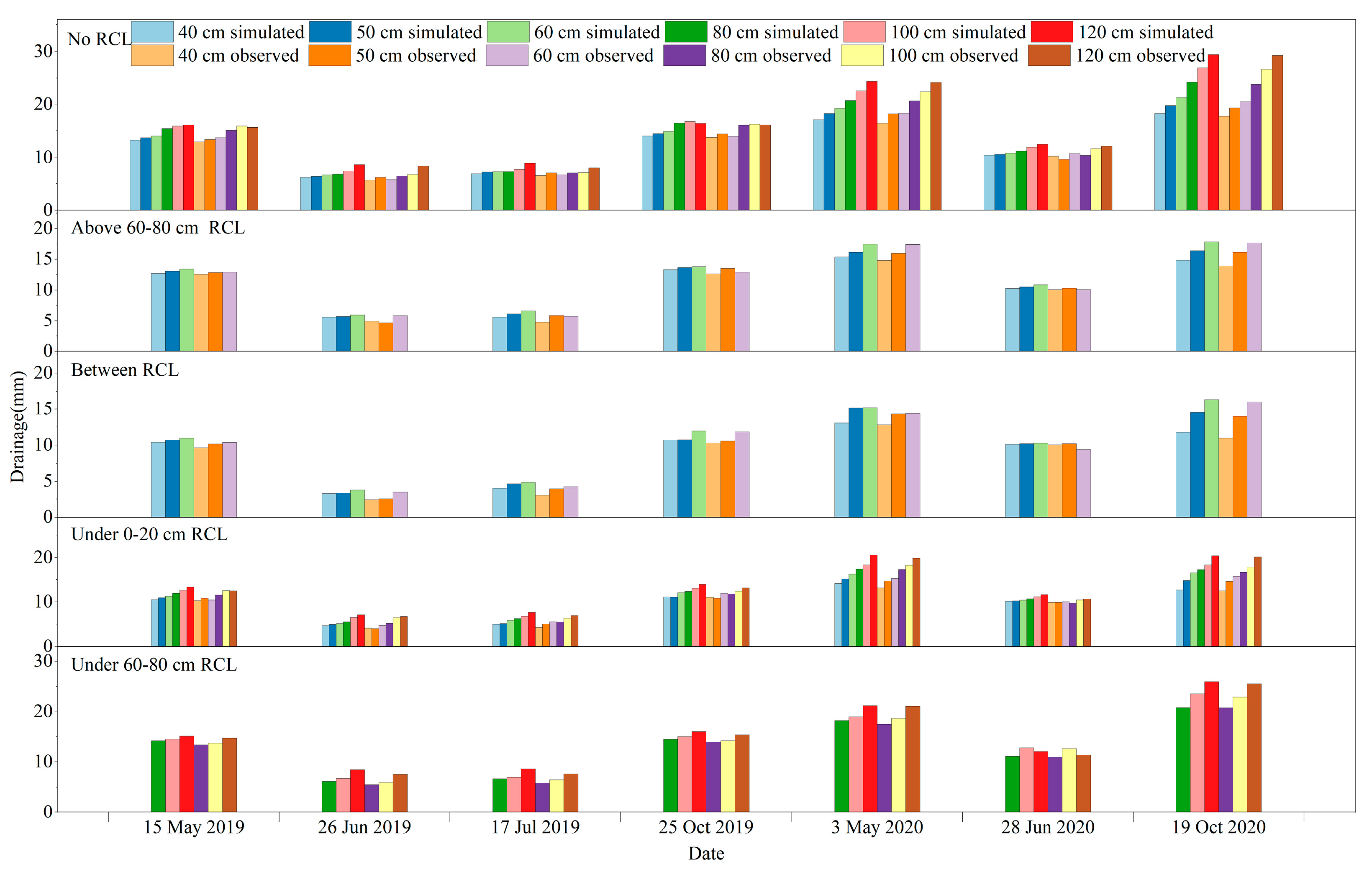
3.2. Effect of the Different RCL Distributions on Subsurface Pipe Drainage

Using the simulation data of the modified DRAINMOD-S model combined with the existing experimental plots, different subsurface pipes were classified according to their distribution positions relative to RCL. The plot had no RCL distribution; the subsurface pipes were located above RCL, the subsurface pipes were located between RCL, and the subsurface pipe was located under the 0–20 cm RCL and under the 60–80 cm RCL in five cases. The subsurface pipe simulation and measured drainage volume after each irrigation in each plot from 2019 to 2020 are shown in Figure 2. Most of the measured subsurface pipe drainage was slightly lower than the simulated drainage. This may be because the model assumes that the process of infiltration from surface water into the subsurface pipe and discharge from farmland is immediate during the simulated subsurface pipe drainage process. In this process, there is no other loss except for water loss that has been included in the model, such as evaporation and transpiration. In the actual irrigation test, other losses will inevitably occur during the process of water infiltration from the farmland into the ground. This may be because the field land is uneven and the channel leaked during the irrigation process. As a result, the actual water entering the test area is lower than the design situation, so the actual measured drainage is slightly lower than the simulated value. This figure shows that under the distribution conditions of various RCL for plots with buried depths of 40, 50, and 60 cm, the water discharge was in the pattern of plots between RCL < under RCL < above RCL < no RCL. For plots with burial depths of 80, 100, and 120 cm, the displacement of plots under the 60–80 cm RCL was significantly higher than that under the 0–20 cm RCL. These results indicate that RCL has an obstructive effect on the drainage of water from the subsurface pipe; the wider the RCL is distributed and the closer it is to the soil surface, the less water is discharged from the subsurface pipe. The water displacement of the plot under the RCL was lower than that above the RCL possibly because the subsurface pipe was located above the RCL, and water accumulated above the RCL. More water was discharged through the subsurface pipe above the RCL, causing water infiltration to decrease. When the subsurface pipe was located under the RCL, some of the water that accumulated above the RCL left the soil via evapotranspiration. The worse the water conductivity of the RCL, the more water evapotranspiration is removed, and the remaining water slowly permeates through the subsurface pipe and discharges.
The unit area water discharge of the subsurface pipe in each plot increased with increasing burial depth, and the unit area drainage increment of each plot differed slightly with increasing burial depth. When the buried depth increases from 40 cm to 60 cm, the unit area water discharge increases by 11.6 mm (no RCL), 13.2 mm (under 0–20 cm RCL), 11.8 mm (above RCL), and 14.2 mm (between RCL). Increasing the burial depth increases the drainage efficiency of the subsurface pipe. The lower the initial water discharge, the greater the increase in water discharge and the more evident the increase in drainage efficiency. This indicates that increasing the burial depth can weaken the ability of the RCL to prevent water infiltration. In the case of the RCL distribution, the drainage efficiency of the subsurface pipe could be improved by increasing the pipe’s buried depth to increase its displacement.

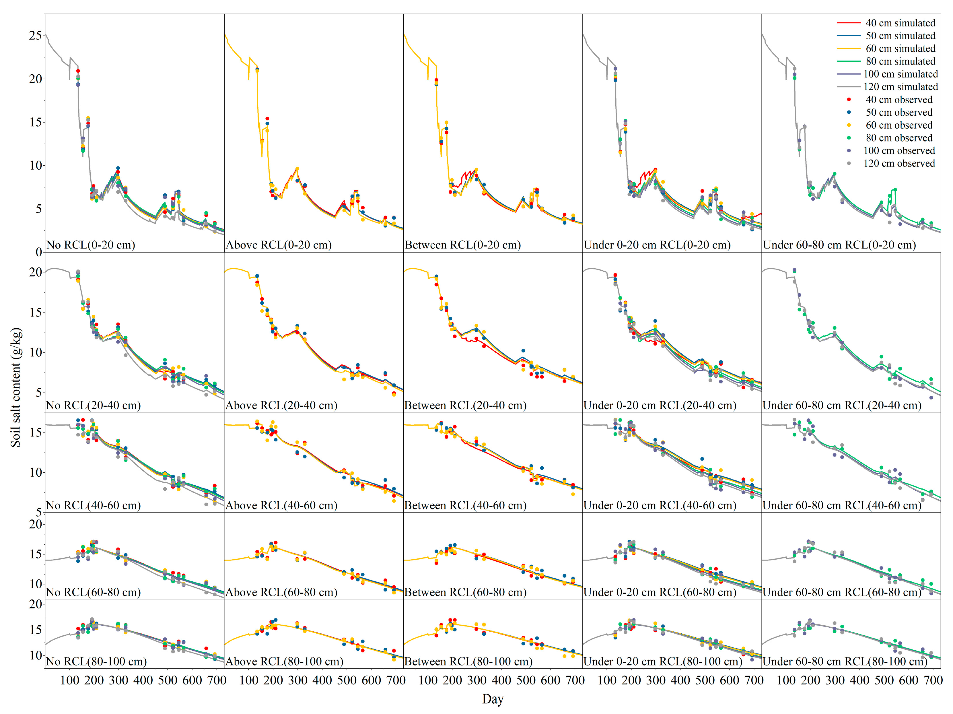
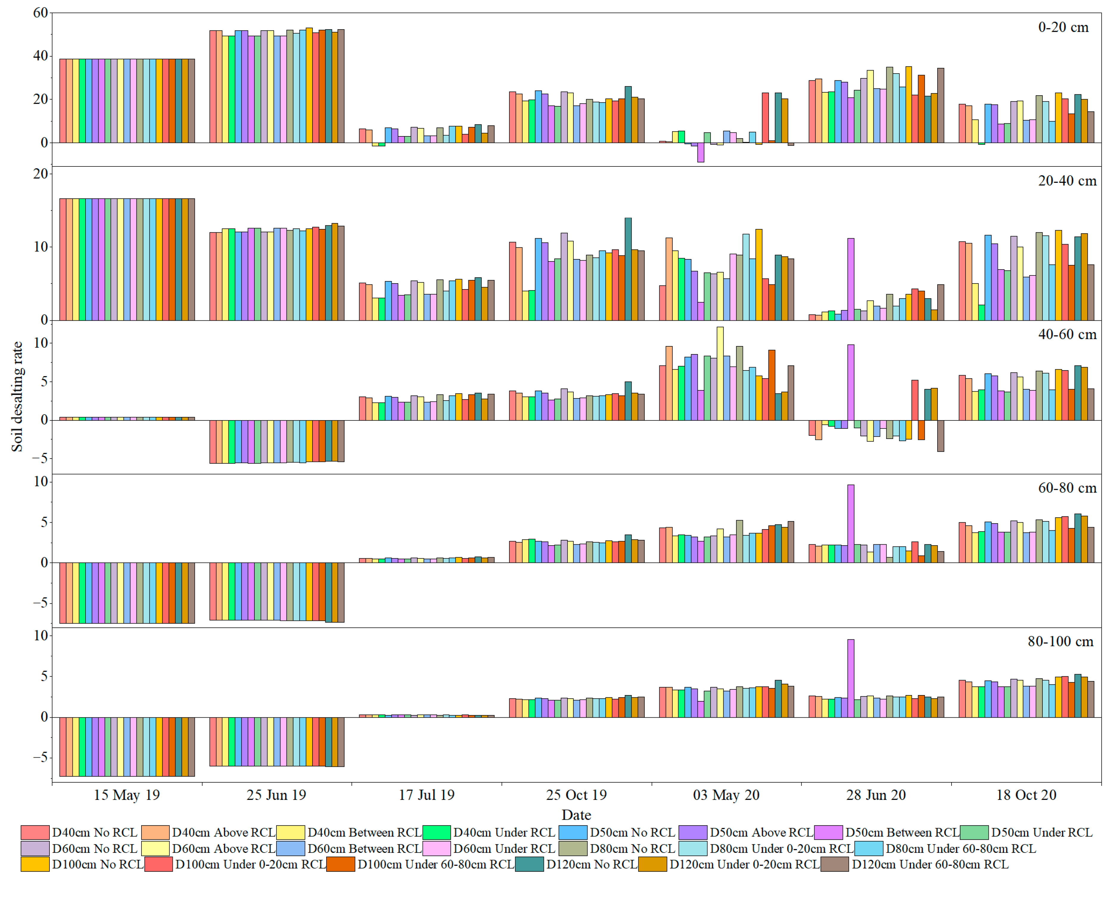
3.3. Effects of the Different RCL Distributions on Soil Salinity and Desalting Rate under Subsurface Pipe Drainage

Figure 3 and Figure 4 show the changes in salt content in different soil layers in each plot and the soil desalting rate after each leaching during 2019–2020. As shown in Figure 3, the simulated and measured values of salt in each soil layer of each plot showed similar trends, and after two years of leaching, soil salinity in all soil layers in the plot with different distributions of RCL decreased considerably. The salt content in the 0–60 cm soil layer in the surface layer showed the most significant change and was accompanied by a slight upward trend at intervals, which was related to evaporation during non-leaching. After a slight increase in salt content, it decreased again under leaching, which was more evident in the 0–20 cm soil layer. In the 60–100 cm soil layer, the salt content increased slightly in the early stage of leaching and gradually decreased in the late stage of leaching in the first year. In the early stages, soil salt infiltrated the deep soil with water, resulting in the accumulation of salt in the deep soil. As the leaching continued, the water content gradually increased. Salt migrated downward from 60 to 100 cm, gradually reducing the salt content in the deep soil. After two years of leaching, the final mean soil salt content of the 0–100 cm soil layer in 40, 50, and 60 cm plots was 6.50 g/kg (no RCL), <6.68 g/kg (above RCL), <7.39 g/kg (under RCL), and <7.45 g/kg (between RCL). After two years of leaching, the final average soil salt content of the 0–100 cm soil layer in 80, 100, and 120 cm plots was 6.32 g/kg (under the 60–80 cm RCL) and <6.77 g/kg (under the 0–20 cm RCL). Water displacement was observed above, as the initial profile of each plot had a very similar salt content. Subsurface pipe drainage, the only drainage method used in this experiment, dissolves salt in water and drains through the subsurface pipe. The more water discharged, the more salt was carried in the water, and the more evident the decrease in the soil salt content.
By comparing the soil desalting rates of each layer in each plot, we found that the desalting rate of each plot increased with increasing burial depth of the subsurface pipe. The average soil desalting rates of the 0–100 cm soil layer in each plot at different burial depths were 6.29% (40 cm) < 6.52% (50 cm) < 6.61% (60 cm) < 6.92% (80 cm) < 7.20% (100 cm) < 7.53% (120 cm). The desalting rates of the different soil layers in each plot were analyzed, and it was found that the rate gradually decreased with increasing depth. The lowest average desalting rate was 18.42% in the soil layer 0–20 cm in all plots, whereas the maximum average desalting rate in the soil layer 80–100 cm was 0.62%. The deeper the soil layer, the worse the leaching effect of the subsurface pipe. Subsurface pipes are more favorable for salt removal from the topsoil. After seven washes over two years, the average soil desalting rate of the 0–100 cm soil layer in the plots with different RCL distribution locations and the same burial depth was as follows: no RCL > above RCL > under RCL > between RCL. At the same burial depth, the soil desalting rate of the subsurface pipe plot at 60–80 cm RCL was higher than that of the subsurface pipe plot at 0–20 cm RCL. Simultaneously, the desalting rate of the soil layers in the plots with RCL was generally lower than that of the corresponding soil layers in the communities without RCL. However, the desalting rates of plots with burial depths of 40, 50, and 60 cm, located above the 60–80 cm RCL, were slightly different. The two-year average soil desalination rate of the 20–60 cm soil layer in the 60–80 cm RCL plot was higher than that of the 20–60 cm soil layer in the non-RCL plot (5.66% > 5.57%). The two-year average soil desalination rate of other soil layers in the 60–80 cm RCL plot was lower than that of the corresponding soil layers in the non-RCL plot (7.93% < 8.01%). This may be because, after most of the irrigation water accumulated above the RCL, a large amount of salt dissolved in the water and drained the soil along the subsurface pipe, resulting in a more evident leaching effect of salt in the upper layer. The 0–20 cm soil layer was located on the surface, and the retention time of water in this layer was short. Moreover, evapotranspiration causes salt accumulation in this layer, which makes it less affected by the RCL. In conclusion, the soil desalting rate of the plot increased with the increasing burial depth of the subsurface pipe. When the subsurface pipe was located above the RCL, the desalting effect was better than when the subsurface pipe was located under the RCL, and the closer it was to the top of the RCL, the better the soil salt leaching effect. When the RCL was distributed above and below, a soil-desalting effect was observed.

4. Discussion

4.1. Effect of the RCL Distribution on Soil Moisture

Many studies on water transport laws in soil, such as subsurface pipe drainage and subsurface water level, have been conducted, but the majority have focused on homogeneous soil. The field soil conditions used in this study differ slightly from those reported in previous studies. The naturally high water retention and low water conductivity of the RCL were similar to those of the addition of a weakly permeable layer to the soil profile. As a result, the infiltration rate of water decreases considerably, resulting in a difference between the change in water in the soil and that without RCL [39,40]. The buried depth of a drainpipe is a crucial factor that affects its drainage capacity. In this study, based on the RCL distribution, the DRAINMOD-S model was used to study the water and salt transport laws under different RCL distributions and subsurface pipe burial depths. According to the design, the RCL was distributed in different positions relative to the subsurface pipe, and increasing the buried depth of the subsurface pipe increased the drainage water of the subsurface pipe. This was the same as the drainage law without RCL distribution [16,41], further explaining that the buried depth of the subsurface pipe has a considerable impact on the drainage efficiency of farmland. The presence of the RCL had a significant influence on the drainage of the subsurface pipe, with the zone containing two layers of the RCL having the lowest drainage. Each additional, weakly permeable layer inevitably further affected the drainage efficiency of the subsurface pipe.
When comparing plots with the same burial depth, the water displacement of the RCL located under the subsurface pipe was 1.29 cm3 lower than that of the RCL located above the pipe over the two years, which was different from the results of Liu et al. [42]. In their study, the drainage rate when the dark pipe was located under RCL was 1.23–1.64 times that when the subsurface pipe was located above RCL. The buried depth of the subsurface pipe in their study was 65 cm, which is similar to the buried depth of the subsurface pipe in this study. This difference in results can be explained by the fact that the test was conducted indoors. Evaporation in the room was much lower than that in the test area (annual evaporation of 2172.5 mm). When water accumulated above the RCL, the water storage depth remained in an area that was greatly affected by evaporation. There was high evaporation in the field, and the rest of the water was either discharged into the subsurface pipe above the RCL, or it penetrated through the RCL into the deep soil. If the pipe was under the RCL, the time taken for water to enter the pipe was prolonged by the influence of the RCL; during the evaporation of water, it greatly increased.

4.2. Effect of the RCL Distribution on Soil Salinity

As salt follows water, the law of soil salt migration is similar to that of water migration under the soil conditions of each plot. When the buried depth of the subsurface pipe increased, the water flux through the subsurface pipe increased, thereby improving the drainage efficiency. Desalting affected the soil profile above the subsurface pipe, which was similar to the results reported by Yang et al. [43], although the desalting rate of the RCL was relatively low [44]. The RCL not only reduced the drainage efficiency, but also reduced the desalting effect of the subsurface pipe, and the salt was hindered by the RCL [45]. The soil desalting rate was in the order of RCL < under RCL < above RCL < no RCL. This rule differs from the results of Liu et al. regarding the salt discharge rate of subsurface pipes under different RCL distributions [42]. When the pipe was located under the RCL, the water carried away by evaporation caused more salt to accumulate at the top of the soil, thus reducing the soil desalination rate. Upon further analysis of the desalting rate of each soil layer, it was found that in the drainage pipes above the 60–80 cm RCL plot, the average of the two-year desalting effect in the 20–60 cm soil layer was considerably better than that of the other layers and was slightly higher than the corresponding depth in the no-RCL plot soil. At the same buried depth as the subsurface pipe, the soil desalting rate at 60–80 cm RCL was higher than that at 0–20 cm RCL. The shallower the distribution of the RCL, the less water enters the soil and evaporates into the atmosphere; therefore, the worse the leaching effect of the soil.
In this study, DRAINMOD-S was successfully used to simulate water and salt transport under complex soil conditions under subsurface drainage conditions. The value of R2 was 0.60–0.90, which proved that DRAINMOD-S was applicable under this condition. Similar to the results of Pourgholam-Amiji et al., DRAINMOD-S has higher simulation accuracy and better performance than AquaCrop, especially under high salt content conditions [24]. Compared with the SWAGMAN Destiny model, DRAINMOD-S is a quasi-two-dimensional model with a wider range of simulation. SWAGMAN Destiny is a point model. Although its accuracy in simulation can also meet the requirements of use, reaching more than 0.5, it has a greater limitation in the spatial simulation analysis of salt, which will bring difficulties to related research [44]. The HYDRUS model is now widely used and has a wide range of applications. It performs well in irrigation experiments with different soil textures [5,43]. However, DRAINMOD-S requires fewer input parameters when simulating subsurface drainage, and the data are easier to obtain [24]. And the simulation results of different soil textures are good, which is similar to the results of this study. This is mainly because DRAINMOD-S is software developed for subsurface drainage. This advantage is that other models cannot be replaced in subsurface simulation. Under comprehensive consideration, the DRAINMOD-S model can be given priority in the simulation of subsurface pipe under complex soil conditions.
In conclusion, for an area with an RCL and high evaporation, the laying depth of the subsurface pipe should be greater than the designated depth with no RCL. When RCL is distributed in the shallow crop root layer, the RCL distributed in the surface layer should be broken by deep ploughing and other methods before improvement or cultivation, which is more conducive to improving the leaching effect of salt [46,47]. When the buried depth of the subsurface pipe is relatively shallow, it should be arranged as far above the RCL as possible according to the local soil conditions, which is conducive to a greater discharge of salt from the soil. Alternatively, other improvement methods should be combined with subsurface pipe drainage to achieve greater drainage effects.

5. Conclusions

In this study, the laws of water and salt migration under different RCL distributions and different buried depths of subsurface pipes were discussed, providing a technical reference for the improvement of subsurface pipes under similar soil conditions around the world. The main conclusions are as follows:
(1)
The area and buried depth of the RCL in the profile affect the accuracy of the model simulation. The calibrated R2, MAE, and RMSE values were 0.60–0.90, 4.31–16.64 cm, and 5.39–17.88 cm, respectively. The NRMSE ranged from 7.36% to 27.08%, and DRAINMOD-S could be used to simulate and predict water and salt transport in the soil.
(2)
In the presence of the RCL, the drainage and salt discharge of the subsurface pipe can be increased by increasing the buried depth of the subsurface pipe to improve the soil desalination rate.
(3)
Under the same buried depth of the subsurface pipe, the amount of drainage and salt discharge when the subsurface pipe is located above the RCL is greater than that when the subsurface pipe is located below the RCL, and the desalination effect is the worst when the RCL is distributed above and below the subsurface pipe simultaneously. The shallower the RCL, the worse the salt drainage effect of the subsurface pipe.

Author Contributions

Writing the initial draft, F.T.; critical review of the work, Q.M.; management and coordination responsibility for the research activity planning and execution, H.S.; writing—review and editing, critical review and revision of the work, R.L.; validation and verification, whether as part of the activity or separately, of the overall replication/reproducibility of results/experiments and other research outputs, J.D.; software, software development, implementation of the computer code and supporting algorithms, testing of existing code components, X.D.; critical revision of the work, W.F. All authors have read and agreed to the published version of the manuscript.

Funding

The 14th Five-Year Key Technologies Research and Development Program (2021YFD1900602-06, H.S.) was financially supported by the Major Science and Technology Projects of Inner Mongolia (zdzx2018059, H.S.), the National Natural Science Foundation of China (52269014, H.S. and 52009056, Q.M.), and the Science and Technology Program of the Inner Mongolia Autonomous Region, China (2022YFHH0044, W.F.).

Data Availability Statement

The data already exist in the manuscript.

Conflicts of Interest

The authors declare that they have no competing financial interests or personal relationships that could have influenced the work reported in this manuscript.

References

  1. Sahab, S.; Suhani, I.; Srivastava, V.; Chauhan, P.S.; Singh, R.P.; Prasad, V. Potential risk assessment of soil salinity to agroecosystem sustainability: Current status and management strategies. Sci. Total Environ. 2021, 764, 144164. [Google Scholar] [CrossRef] [PubMed]
  2. Kerschbaumer, L.; Kobbing, J.F.; Ott, K.; Zerbe, S.; Thevs, N. Development scenarios on Hetao irrigation area (China): A qualitative analysis from social, economic and ecological perspectives. Environ. Earth Sci. 2015, 73, 815–834. [Google Scholar] [CrossRef]
  3. Chang, X.; Gao, Z.; Wang, S.; Chen, H. Modelling long-term soil salinity dynamics using SaltMod in Hetao irrigation district, China. Comp. Electron. Agric. 2019, 156, 447–458. [Google Scholar] [CrossRef]
  4. Feng, Z.Z.; Miao, Q.F.; Shi, H.B.; Feng, W.Y.; Li, X.Y.; Yan, J.W.; Liu, M.H.; Sun, W.; Dai, L.P.; Liu, J. Simulation of water balance and irrigation strategy of typical sand-layered farmland in the Hetao Irrigation District, China. Agric. Water Manag. 2023, 280, 108236. [Google Scholar] [CrossRef]
  5. Dou, X.; Shi, H.B.; Li, R.P.; Miao, Q.F.; Yan, J.W.; Tian, F.; Wang, B. Simulation and evaluation of soil water and salt transport under controlled subsurface drainage using HYDRUS-2D model. Agric. Water Manag. 2022, 273, 107899. [Google Scholar] [CrossRef]
  6. Feng, W.Y.; Wang, T.K.; Zhu, Y.R.; Sun, F.H.; Giesy, J.P.; Wu, F.C. Chemical composition, sources, and ecological effect of organic phosphorus in water ecosystems: A review. Carbon Res. 2023, 2, 12. [Google Scholar] [CrossRef]
  7. Feng, W.Y.; Yang, F.; Cen, R.; Liu, J.; Qu, Z.Y.; Miao, Q.F.; Chen, H.Y. Effects of straw biochar application on soil temperature, available nitrogen and growth of corn. J. Environ. Manag. 2021, 277, 111331. [Google Scholar] [CrossRef]
  8. Zhou, L.X.; Liu, W.; Duan, H.J.; Dong, H.W.; Li, J.C.; Zhang, S.X.; Zhang, J.; Ding, S.G.; Xu, T.Y.; Guo, B.B. Improved effects of combined application of nitrogen-fixing bacteria Azotobacter beijerinckii and microalgae Chlorella pyrenoidosa on wheat growth and saline-alkali soil quality. Chemosphere 2023, 313, 137409. [Google Scholar] [CrossRef]
  9. Sun, Z.W.; Ge, J.M.; Li, C.; Wang, Y.P.; Zhang, F.Z.; Lei, X.D. Enhanced improvement of soda saline-alkali soil by in-situ formation of super-stable mineralization structure based on CaFe layered double hydroxide and its large-scale application. Chemosphere 2022, 300, 134543. [Google Scholar] [CrossRef]
  10. Haj-Amor, Z.; Bouri, S. Subsurface drainage system performance, soil salinization risk, and shallow groundwater dynamic under irrigation practice in an arid land. Arabian J. Sci. Eng. 2018, 44, 467–477. [Google Scholar] [CrossRef]
  11. Askar, M.H.; Youssef, M.A.; Chescheir, G.M.; Negm, L.M.; King, K.W.; Hesterberg, D.L.; Amoozegar, A.; Skaggs, R.W. DRAINMOD Simulation of macropore flow at subsurface drained agricultural fields: Model modification and field testing. Agric. Water Manag. 2020, 242, 106401. [Google Scholar] [CrossRef]
  12. Revuelta-Acosta, J.D.; Flanagan, D.C.; Engel, B.A.; King, K.W. Improvement of the Water Erosion Prediction Project (WEPP) model for quantifying field scale subsurface drainage discharge. Agric. Water Manag. 2021, 244, 106597. [Google Scholar] [CrossRef]
  13. Takeshima, R.; Murakami, S.; Fujiwara, Y.; Nakano, K.; Fuchiyama, R.; Hara, T.; Shima, T.; Koyama, T. Subsurface drainage and raised-bed planting reduce excess water stress and increase yield in common buckwheat (Fagopyrum esculentum Moench). Field Crops Res. 2023, 297, 108935. [Google Scholar] [CrossRef]
  14. Pan, P.; Qi, Z.M.; Zhang, T.Q.; Ma, L.W. Modeling phosphorus losses to subsurface drainage under tillage and compost management. Soil Tillage Res. 2023, 227, 105587. [Google Scholar] [CrossRef]
  15. Tao, Y.; Li, N.; Wang, S.; Chen, H.; Guan, X.; Ji, M. Simulation study on performance of nitrogen loss of an improved subsurface drainage system for onetime drainage using HYDRUS-2D. Agric. Water Manag. 2021, 246, 106698. [Google Scholar] [CrossRef]
  16. Qian, Y.Z.; Zhu, Y.; Ye, M.; Huang, J.S.; Wu, J.W. Experiment and numerical simulation for designing layout parameters of subsurface drainage pipes in arid agricultural areas. Agric. Water Manag. 2021, 243, 106455. [Google Scholar] [CrossRef]
  17. Yoon, K.S.; Choi, J.K.; Son, J.G.; Cho, J.Y. Concentration profile of nitrogen and phosphorus in leachate of a paddy plot during the rice cultivation period in southern Korea. Commun. Soil Sci. Plant Anal. 2006, 37, 1957–1972. [Google Scholar] [CrossRef]
  18. Kale, S. Field-evaluation of DRAINMOD-S for predicting soil and drainage water salinity under semi-arid conditions in Turkey. Span. J. Agric. Res. 2011, 9, 1142–1155. [Google Scholar] [CrossRef]
  19. Hashemi, S.; Darzi-Naftchali, A.; Qi, Z.M. Assessing water and nitrate-N losses from subsurface-drained paddy lands by DRAINMOD-N II. Irrig. Drain. 2020, 69, 776–787. [Google Scholar] [CrossRef]
  20. Bou Lahdou, G.; Bowling, L.; Frankenberger, J.; Kladivko, E. Hydrologic controls of controlled and free draining subsurface drainage systems. Agric. Water Manag. 2019, 213, 605–615. [Google Scholar] [CrossRef]
  21. Kaur, H.; Nelson, K.A.; Singh, G.; Veum, K.S.; Davis, M.P.; Udawatta, R.P.; Kaur, G. Drainage water management impacts soil properties in floodplain soils in the midwestern, USA. Agric. Water Manag. 2023, 279, 108193. [Google Scholar] [CrossRef]
  22. Hay, C.H.; Reinhart, B.D.; Frankenberger, J.R.; Helmers, M.J.; Jia, X.; Nelson, K.A.; Youssef, M.A. Frontier: Drainage water recycling in the humid regions of the US: Challenges and opportunities. Trans. ASABE 2021, 64, 1095–1102. [Google Scholar] [CrossRef]
  23. Singh, G.; Nelson, K.A. Long-term drainage, subirrigation, and tile spacing effects on maize production. Field Crops Res. 2021, 262, 108032. [Google Scholar] [CrossRef]
  24. Pourgholam-Amiji, M.; Liaghat, A.; Ghameshlou, A.N.; Khoshravesh, M. The evaluation of DRAINMOD-S and AquaCrop models for simulating the salt concentration in soil profiles in areas with a saline and shallow water table. J. Hydrol. 2021, 598, 126259. [Google Scholar] [CrossRef]
  25. Ghane, E.; Askar, M.H. Predicting the effect of drain depth on profitability and hydrology of subsurface drainage systems across the eastern USA. Agric. Water Manag. 2021, 258, 107072. [Google Scholar] [CrossRef]
  26. Moursi, H.; Youssef, M.A.; Chescheir, G.M. Development and application of DRAINMOD model for simulating crop yield and water conservation benefits of drainage water recycling. Agric. Water Manag. 2022, 266, 107592. [Google Scholar] [CrossRef]
  27. Awad, A.; Luo, W.; El-Rawy, M. Improvement of the DRAINMOD model’s performance under time-variable surface storage capacities using neural network models. Ain Shams Eng. J. 2022, 13, 101699. [Google Scholar] [CrossRef]
  28. Lisenbee, W.A.; Hathaway, J.M.; Winston, R.J. Modeling bioretention hydrology: Quantifying the performance of DRAINMOD-Urban and the SWMM LID module. J. Hydrol. 2022, 612, 128179. [Google Scholar] [CrossRef]
  29. D’Angelo, B.; Bruand, A.; Qin, J.; Peng, X.; Hartmann, C.; Sun, B.; Hao, H.; Rozenbaum, O.; Muller, F. Origin of the high sensitivity of Chinese red clay soils to drought: Significance of the clay characteristics. Geodermas 2014, 223–225, 46–53. [Google Scholar] [CrossRef]
  30. Tong, W.; Chen, X.; Wen, X.; Chen, F.; Zhang, H.; Chu, Q.; Dikgwatlhe, S. Applying a salinity response function and zoning saline land for three field crops: A case study in the Hetao Irrigation District, Inner Mongolia, China. J. Integr. Agric. 2015, 14, 178–189. [Google Scholar] [CrossRef]
  31. Skaggs, R.W. Combination surface-subsurface drainage systems for humid regions. J. Irrig. Drain. Div. Am. Soc. Civil Eng. 1980, 106, 265–283. [Google Scholar] [CrossRef]
  32. Green, W.H.; Ampt, G.A. Studies on Soil Phyics. J. Agric. Sci. 1911, 4, 1–24. [Google Scholar] [CrossRef]
  33. Kirkham, D. Theory of land drainag. In Drainage of Agricultural Lands, Agronomy Monograph 7; Luthin, J.N., Ed.; American Society of Agronomy: Madison, WI, USA, 1957; pp. 139–181. [Google Scholar]
  34. Skaggs, R.W.; Youssef, M.A.; Chescheir, G.M. DRAINMOD: Model use, calibration, and validation. Trans. ASABE 2012, 55, 1509–1522. [Google Scholar] [CrossRef]
  35. FAO. Crop Evapotranspiration, Guidelines for Computing Crop Water Requirements; Irrig Drain Paper No. 56; FAO: Rome, Italy, 1998. [Google Scholar]
  36. Thornthwaite, C.W. An Approach toward a Rational Classification of Climate. Geogr. Rev. 1948, 38, 55–94. [Google Scholar] [CrossRef]
  37. Bannayan, M.; Hoogenboom, G. Using pattern recognition for estimating cultivar coefficients of a crop simulation model. Field Crops Res. 2009, 111, 290–302. [Google Scholar] [CrossRef]
  38. Masasi, B.; Taghvaeian, S.; Gowda, P.H.; Marek, G.; Boman, R. Validation and application of AquaCrop for irrigated cotton in the Southern Great Plains of US. Irrig. Sci. 2020, 38, 593–607. [Google Scholar] [CrossRef]
  39. Li, Y.; Zhang, H.B.; Fu, C.C.; Tu, C.; Luo, Y.M.; Christie, P. A red clay layer in soils of the Yellow River Delta: Occurrence, properties and implications for elemental budgets and biogeochemical cycles. Catena 2019, 172, 469–479. [Google Scholar] [CrossRef]
  40. Xin, P.; Dan, H.-C.; Zhou, T.; Lu, C.; Kong, J.; Li, L. An analytical solution for predicting the transient seepage from a subsurface drainage system. Adv. Water Resour. 2016, 91, 1–10. [Google Scholar] [CrossRef]
  41. Muhammad, E.; Ibrahim, M.; El-Sayed, A. Effects of drain depth on crop yields and salinity in subsurface drainage in Nile Delta of Egypt. Ain Shams Eng. J. 2021, 12, 1595–1606. [Google Scholar] [CrossRef]
  42. Liu, Y.; Ao, C.; Zeng, W.; Kumar Srivastava, A.; Gaiser, T.; Wu, J.; Huang, J. Simulating water and salt transport in subsurface pipe drainage systems with HYDRUS-2D. J. Hydrol. 2021, 592, 125823. [Google Scholar] [CrossRef]
  43. Yang, T.; Šimůnek, J.; Mo, M.; Mccullough-Sanden, B.; Shahrokhnia, H.; Cherchian, S.; Wu, L. Assessing salinity leaching efficiency in three soils by the HYDRUS-1D and -2D simulations. Soil Tillage Res. 2019, 194, 104342. [Google Scholar] [CrossRef]
  44. Yang, H.; Chen, Y.; Zhang, F.; Xu, T.; Cai, X. Prediction of salt transport in different soil textures under drip irrigation in an arid zone using the SWAGMAN Destiny model. Soil Res. 2016, 54, 869–879. [Google Scholar] [CrossRef]
  45. Chen, L.; Feng, Q.; Wang, Y.; Yu, T. Water and salt movement under saline water irrigation in soil with clay interlayer. Trans. Chin. Soc. Agric. Eng. 2012, 28, 44–51, (In Chinese with English Abstract). [Google Scholar]
  46. Yao, R.; Gao, Q.C.; Liu, Y.X.; Li, H.Q.; Yang, J.S.; Bai, Y.C.; Zhu, H.; Wang, X.P.; Xie, W.P.; Zhang, X. Deep vertical rotary tillage mitigates salinization hazards and shifts microbial community structure in salt-affected anthropogenic-alluvial soil. Soil Tillage Res. 2023, 227, 105627. [Google Scholar] [CrossRef]
  47. Wu, F.; Zhai, L.C.; Xu, P.; Zhang, Z.B.; Elamin, H.B.; Lemessa, N.T.; Roy, N.K.; Jia, X.L.; Guo, H.Q. Effects of deep vertical rotary tillage on the grain yield and resource use efficiency of winter wheat in the Huang-Huai-Hai Plain of China. J. Integr. Agric. 2021, 20, 593–605. [Google Scholar] [CrossRef]
Figure 1. Buffer lines of pipeline laying and distribution of the red clay layer (RCL).
Agronomy 14 00017 g001
Figure 2. Simulated and observed subsurface pipe drainage volume of each plot from 2019 to 2020. (RCL is the red clay layer).
Agronomy 14 00017 g002
Figure 3. Changes in soil salt content in each soil layer of each experimental plot were simulated and observed during 2019–2020. (RCL is the red clay layer).
Agronomy 14 00017 g003
Figure 4. Simulated values of soil desalination rate in each soil layer after each irrigation in each experimental plot from 2019 to 2020. (RCL is the red clay layer; D is the subsurface pipe depth).
Agronomy 14 00017 g004
Table 1. Physical and chemical characteristics of soil at the experimental site.
Depth (cm)Particle Composition/%Soil TextureBulk Density
(g·cm−3)
Soil Salt Content
(g·kg−1)
Field Capacity
(cm3 cm−3)
Saturated Hydraulic Conductivity
(cm·day−1)
SandClaySilt
0–209.469.0481.50Silt1.4623.5133.081.92
20–4021.9812.5165.51Silt loam1.4618.2235.223.12
40–6025.2714.1460.59Silt loam1.4915.5335.533.36
60–803.3610.7085.94Silt1.5011.7936.192.16
80–10025.9113.3760.72Silt loam1.5110.6036.713.59
Table 2. Key input parameters of the DRAINMOD-S model.
Parameter TypeConcrete Parameters (Degree of Sensitivity)Calibration Parameter ValuesUnit
ClimateMaximum and minimum daily temperaturesThe micro weather station (HOBO-U30)°C
Amount of rain dailyThe micro weather station (HOBO-U30)mm
PETPenman–Monteithmm
SoilSaturated hydraulic conductivity
(0–20 cm, RCL, highly sensitive)
0.5mm/h
Saturated hydraulic conductivity
(20–40 cm, highly sensitive)
1.1mm/h
Saturated hydraulic conductivity
(40–60 cm, highly sensitive)
1.3mm/h
Saturated hydraulic conductivity
(60–80 cm, RCL, highly sensitive)
0.7mm/h
Saturated hydraulic conductivity
(80–100 cm, highly sensitive)
1.2mm/h
Depth of impenetrable layer (light-sensitive)200cm
Initial soil salinityField measured values (Table 1)g/kg
Drainage systemDrainage depth (sensitive)Layout of each test plotcm
Drainage spacing (sensitive)1000cm
Effective drainage radius (non-sensitive)1.5cm
Maximum surface water storage depth 18cm
Initial groundwater level depth (sensitive)160cm
Drainage coefficient (non-sensitive)14mm/day
Kirkham’s depth for flow to drains0.3cm
WaterAmount of irrigation waterActual irrigation quotam3/ha
Average of irrigation water salinity0.67g/L
Table 3. Model hydrologic simulation performance statistics in 2019 (calibration) and 2020 (validation).
Depth
(cm)
RCL
(cm)
2019 (Calibration)2020 (Validation)
R2 (-)MAE (cm)RMSE (cm)NRMSER2 (-)MAE (cm)RMSE (cm)NRMSE
80-0.92 7.027.399.35%0.91 6.837.3814.07%
0–200.90 12.8813.6015.76%0.83 10.7311.9722.01%
60–800.90 8.229.5511.97%0.89 6.157.0215.47%
0–20 and 60–800.858.9110.3412.62%0.8014.6016.3527.15%
100-0.91 5.065.837.47%0.88 5.956.6712.68%
0–200.88 10.6012.6714.90%0.82 6.949.4216.35%
60–800.89 7.939.1911.49%0.84 9.4210.6220.46%
0–20 and 60–800.83 14.0615.5717.72%0.7713.2214.2324.25%
120-0.89 5.566.798.39%0.86 6.206.4513.33%
0–200.85 9.3710.4812.32%0.80 15.5916.5524.05%
60–800.88 8.339.0610.98%0.82 7.298.4317.99%
0–20 and 60–800.8414.8416.1017.93%0.73 19.1220.1529.37%
Note: RCL, red clay layer; R2, coefficient of determination; MAE, mean absolute error; RMSE, root mean square error; NRMSE, normalized root mean square error. Four treatments: no RCL, 0–20 cm or 60–80 cm RCL, 0–20 cm RCL, and 60–80 cm RCL. Data on 15 May, 26 June, 17 July, 25 October 2019 were used for calibration. Data on 3 May, 28 June, 19 October 2020 were used for validation.
Table 4. Model salt simulation performance statistics in 2019 (calibration) and 2020 (validation).
Depth
(cm)
RCL
(cm)
2019 (Calibration)2020 (Validation)
R2 (-)MAE (g/kg)RMSE (g/kg)NRMSER2 (-)MAE (g/kg)RMSE (g/kg)NRMSE
80-0.90 5.476.127.90%0.90 7.037.1313.54%
0–200.85 10.5412.3214.68%0.70 10.2612.0322.30%
60–800.88 8.819.5111.82%0.88 7.148.3718.05%
0–20 and 60–800.8213.9615.7918.16%0.6313.8014.5124.42%
100-0.90 4.685.717.36%0.84 4.315.3910.57%
0–200.85 13.8114.9916.97%0.73 12.7714.2422.46%
60–800.87 6.978.5810.85%0.82 11.0711.4521.39%
0–20 and 60–800.82 16.6417.8819.76%0.6712.5815.3126.38%
120-0.90 8.428.9710.70%0.81 8.388.9317.67%
0–200.84 12.7214.2616.14%0.75 10.4211.9118.71%
60–800.87 13.5614.4516.48%0.83 10.5410.9721.89%
0–20 and 60–800.8214.5216.7818.75%0.60 13.2016.9727.08%
Note: RCL, red clay layer; R2, coefficient of determination; MAE, mean absolute error; RMSE, root mean square error; NRMSE, normalized root mean square error. Four treatments: no RCL, 0–20 cm or 60–80 cm RCL, 0–20 cm RCL, and 60–80 cm RCL.
Disclaimer/Publisher’s Note: The statements, opinions and data contained in all publications are solely those of the individual author(s) and contributor(s) and not of MDPI and/or the editor(s). MDPI and/or the editor(s) disclaim responsibility for any injury to people or property resulting from any ideas, methods, instructions or products referred to in the content.

