Article

The Nondestructive Model of Near-Infrared Spectroscopy with Different Pretreatment Transformation for Predicting “Dangshan” Pear Woolliness Disease

1
College of Economics and Management, Anhui Agricultural University, Hefei 230001, China
2
College of Horticulture, Anhui Agricultural University, Hefei 230001, China
3
College of Information and Computer Science, Anhui Agricultural University, Hefei 230001, China
4
Key Laboratory of Agricultural Sensors, Ministry of Agriculture and Rural Affairs, Anhui Agricultural University, Hefei 230001, China
*
Author to whom correspondence should be addressed.
Agronomy 2023, 13(5), 1420; https://doi.org/10.3390/agronomy13051420
Submission received: 23 April 2023 / Revised: 18 May 2023 / Accepted: 19 May 2023 / Published: 20 May 2023
(This article belongs to the Special Issue The Application of Near-Infrared Spectroscopy in Agriculture)

Abstract

:
The “Dangshan” pear woolliness response is a physiological disease that mostly occurs in the pear growth process. The appearance of the disease is not obvious, and it is difficult to detect with the naked eye. Therefore, finding a way to quickly and nondestructively identify “Dangshan” pear woolliness disease is of great significance. In this paper, the near-infrared spectral (NIR) data of “Dangshan” pear samples were collected at 900–1700 nm reflectance spectra using a handheld miniature NIR spectrometer, and the data were modelled and analysed using random forest (RF), support vector machine (SVM) and boosting algorithms under the processing of 24 pretreatment methods. Considering the variations between different pretreatment methods, this work determined the relative optimality index of different pretreatment methods by evaluating their effects on model accuracy and Kappa and selected the best-performing first derivative with standard normal variate and Savitzky–Golay and first derivative with multiplicative scatter correction and Savitzky–Golay as the best pretreatment methods. With the best pretreatment method, all five models in the three categories showed good accuracy and stability after parameter debugging, with accuracy and F1 greater than 0.8 and Kappa floating at approximately 0.7, reflecting the good classification ability of the models and proving that near-infrared spectroscopy (NIRS) in the rapid identification of “Dangshan” pear woolliness response disease was feasible. By comparing the performance differences of the models before and after the pretreatment methods, it was found that the ensemble-learning models such as RF and boosting were more stringent on pretreatment methods in identifying “Dangshan” pear woolliness response disease than support vector machines, and the performance of the ensemble learning models was significantly improved under appropriate pretreatment methods. This experiment provided a relatively stable detection method for “Dangshan” pear woolliness response disease under nonideal detection conditions by analysing the impact of pretreatment methods and models on the prediction result.

1. Introduction

Pear is a cultivated fruit tree belonging to the Rosaceae family and is the second most productive fruit crop, having been farmed worldwide for more than five thousand years [1]. As a widely grown and eaten fruit [2,3], there are many different kinds of pears, and there are significant natural differences between different kinds [4,5], among which the Chinese “Dangshan” pear is liked by consumers for its bright yellow color, crispness, sweetness, and juiciness. Pear trees are susceptible to various diseases during the growing process, not only threatening the growth of the pear tree but also affecting the quality of the pear fruit. Among these diseases, the woolliness response of pear can cause a decrease in the quality and taste of the fruit, leading to a decline in the reputation of “Dangshan” pear and causing certain economic losses for fruit farmers. Hence, to reduce the economic losses caused to fruit farmers by the outbreak of “Dangshan” pear woolliness response disease (DPWD), it is important to detect infected fruits in a timely manner and take corresponding preventive measures.
The “Dangshan” pear woolliness response is a physiological disease and is connected with the deficit of elements such as boron and calcium and water loss during the growth of pear trees [6,7]. The DPWD generally arises in orchards with late picking, higher average single fruit (more than 400 g), dry weather before harvest, excessive tree load, excessive use of nitrogen fertilizer or calcium deficiency. Diseased fruits show a rough appearance on the surface with thickened skin, dark yellow color, and internal dehydration. The hardness decreases, the flesh becomes loose, and serious cases result in sponge-like texture.
In the process of identifying DPWD, the traditional manual method has high costs, low identification accuracy, and a long working period in identification due to the large sample base and inconspicuous appearance of the disease, which does not meet the requirements of modern agriculture. Thus, it is vital to discover a fast, low-cost, and high-accuracy identification approach for the detection of DPWD. In recent years, the application of near-infrared spectroscopy became increasingly mature in the field of agricultural product quality testing because of its nonpolluting simple operation and lack of damage to the sample during the testing process [8,9,10]. In our team’s research, WenJing Ba and Lianglong Wang modelled and analysed the nutritional deficiencies in pear leaves and Fusarium head blight in wheat grains using near-infrared spectroscopy [11,12,13], accumulating experience for other team members in modelling and analysing using near-infrared spectroscopy. Therefore, this paper uses near-infrared spectroscopy to establish an identification model for DPWD and discusses the feasibility of using near-infrared spectroscopy for the diagnosis of DPWD.
Near-infrared spectra belong to the multiplicative and principal frequency absorption spectra of molecular vibrations, which are highly penetrating due to the non-resonant nature of molecular vibrations, mainly generated when the molecular vibrations jump from the ground state to higher energy levels. NIR light is mainly the multiplicative and ensemble frequency absorption of X-H (X = C, N, O) vibrations of hydrogen-containing groups [14], and different groups have different energy levels. Different groups and the same group in different physicochemical environments absorb NIR light at significantly different wavelengths, so NIR spectra can be used as an effective vehicle for obtaining information. Because the water content of diseased fruit is significantly absent compared to normal fruit, the woolliness condition of pears can be judged by measuring the absorption of O-H groups in the spectra.
To make “true” chemical correlations between spectral data and O-H groups, improving the performance and accuracy of the model, various pretreatment methods were used in this experiment to correct the data for scattering, baseline variations, peak shifts, noise, missing values, and other artifacts [15]. Various pretreatment methods affect the data in different ways to different degrees, and pretreatment methods always entail the risk of losing relevant chemical information or changes linked to the attributes of interest [16,17,18]. However, combinations of different pretreatment methods can attenuate or remove the effect of a single pretreatment method on the spectral information. Therefore, seven pretreatment methods and their 16 common pretreatment combinations were selected in this paper to process near-infrared spectra to find pretreatment methods that both attenuate noise and scattering in the data and retain the maximum amount of spectral information [19].
To improve the classification ability of the model on the problem of identifying DPWD and to provide a more reliable reference for practical production, this paper improves the performance of the model through the selection of pretreatment methods and the debugging of model parameters. In the second section of this paper, the samples and tools used in the experiments are introduced, including the pretreatment methods, classification algorithms, and evaluation metrics of the models. Section 3 then shows the specific process of the experiment, including the selection of pretreatment and optimization of the model, and conclusions from the experiment are presented in Section 4.
Team member Yuanfeng Chen achieved excellent results in predicting DPWD by integrating the near-infrared spectroscopy data and features of corresponding sample images of “Dangshan” pear [20], based on the near-infrared spectroscopy data and images of “Dangshan” pear. However, in the process of collecting pear fruit sample photos, stable light sources and professional shooting equipment are needed, which are difficult to obtain in actual agricultural production. The purpose of this experiment is to compare different pretreatment methods and models during the detection process to select a model with good predictive ability when using near-infrared spectroscopy data for prediction. This is necessary to enable fast and stable detection of DPWD under restricted usage scenarios.

2. Materials and Methods
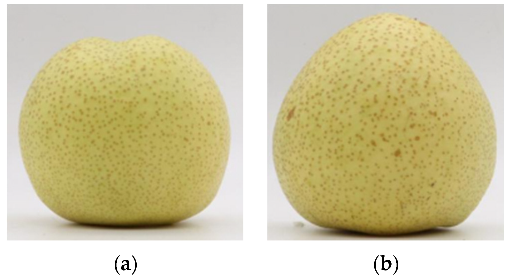
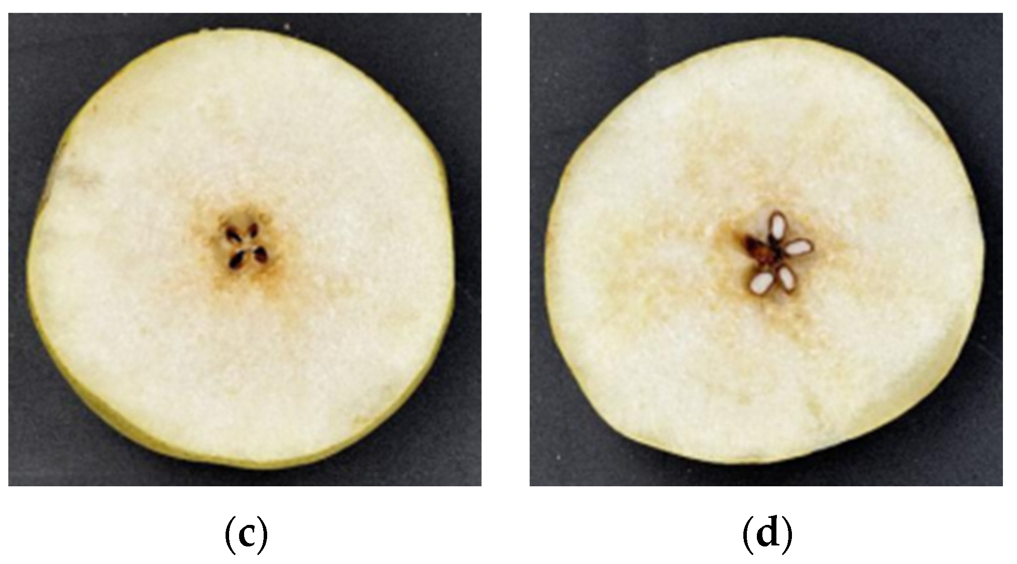
2.1. Sample Sources

The tested pear trees in this experiment were “Dangshan” pear trees in Yeji District, Lu’an City, Anhui Province, with uniform plant growth and robust growth. The city boundary lies between 115°20′~17°14′ E and 31°01′~32°40′ N, which belongs to the transition zone from the north subtropical to warm temperate zone, with a spectacular monsoon, four different seasons, pleasant climate, copious rainfall, and ample light. However, due to the transition zone from north subtropical to warm temperate zone, the warm and cold air currents meet frequently, and the monsoon varies in strength between years, with different advancement and retreat, resulting in variable climate, often threatened by water and drought disasters, and many factors restricting agricultural production. The “Dangshan” pear garden area of Youjia Agricultural Development Co., Ltd. contains good soil (yellow loam; the pH value is approximately 6.8–7.4; clay), which is suitable for the growth of pear trees. In 2022, the DPWD appeared on the “Dangshan” pear trees in the park. Representative samples were selected from both the infected and healthy trees, resulting in a total of 240 pears collected from each group in early September. Before conducting the experiment, we thoroughly cleaned and wiped the surface of each pear, and made numbered backups. Figure 1 shows the comparison of healthy and diseased samples.
As shown in Figure 1, the profiles of diseased samples and healthy samples were obviously different. The profile of the diseased sample showed a yellow pattern, low water content, and poor hardness; therefore, we can judge whether the predicted results of the model are correct by comparing the profile of the sample with the predicted results of the model.

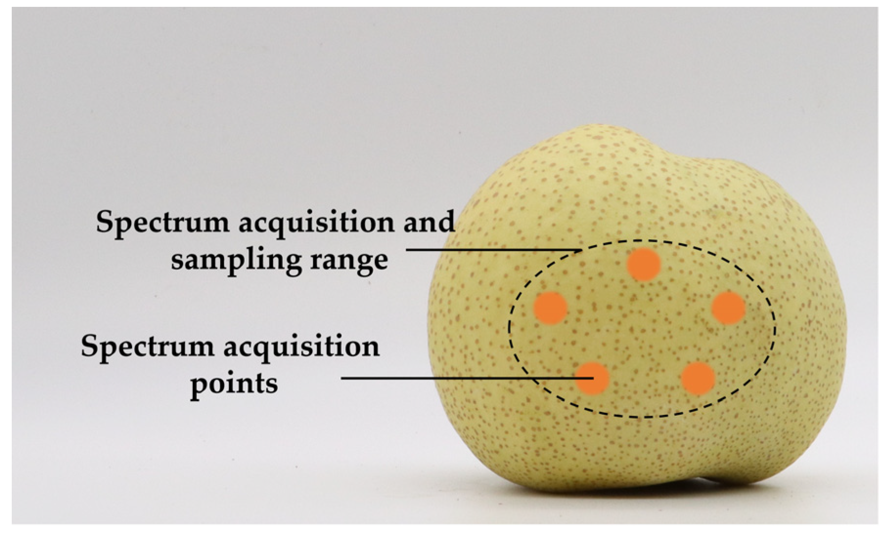
2.2. Experimental Apparatus and Data Acquisition

In this experiment, the instrument used to collect the spectral data was a handheld miniature NIR spectrometer with the model number “NIR-S-G1” produced by Shenzhen Green Union Company. The spectral wavelength detection range was 900 nm~1700 nm, the spectral acquisition points were 228 bands, the spectral resolution was 3.89 nm, and the signal-to-noise ratio (SNR) was 5000:1, as shown in Figure 2.
Before using the handheld miniature NIR spectrometer, the “Instagram” application on the phone was connected to the instrument via Bluetooth, and then, sample spectral data were acquired. Before each measurement, the NIR spectrometer was calibrated using a black and white board. The instrument was pressed against the calibration white board, and the emitted light was reflected by the white board and captured and recorded as the brightness value (W) of the white board. Then, the emitted light source of the instrument was turned off, and the brightness value (B) on the black board was recorded at this time. After calibrating the instrument, the spectral data of the pear fruit surface began to be gathered, the light source window of the instrument was placed close to the “Dangshan” pear sample, and the reflected light acquired was recorded as the brightness value (R) of the pear surface. The spectral reflectance of the sample was estimated according to Formula (1), where the luminance value (I) was the original luminance value of the instrument.
R = ( I B ) ( W B ) × 100 %
Before collecting the spectral data, an ellipse with a short axis of approximately 3 cm and a long axis of approximately 5 cm was delineated with a pencil at 120° intervals near the equator of the normal fruit peel surface, and the area within the ellipse was used as the range for spectral data collection; the two ends and the center part of the central axis of the area were used as the range for spectral collection. The scanning window at the front end of the mini handheld spectrometer was placed close to the delineated area, and each sample area was scanned 5 times. Each data file was named according to the sample number. After the spectral data collection was completed, all files were exported, and the data in each file included wavelength, intensity spectrum, absorbance spectrum, and reflectance. The average of reflectance spectral data from 5 scans in each area was used as the original modelling spectral data, and the five-point distribution is shown in Figure 3.

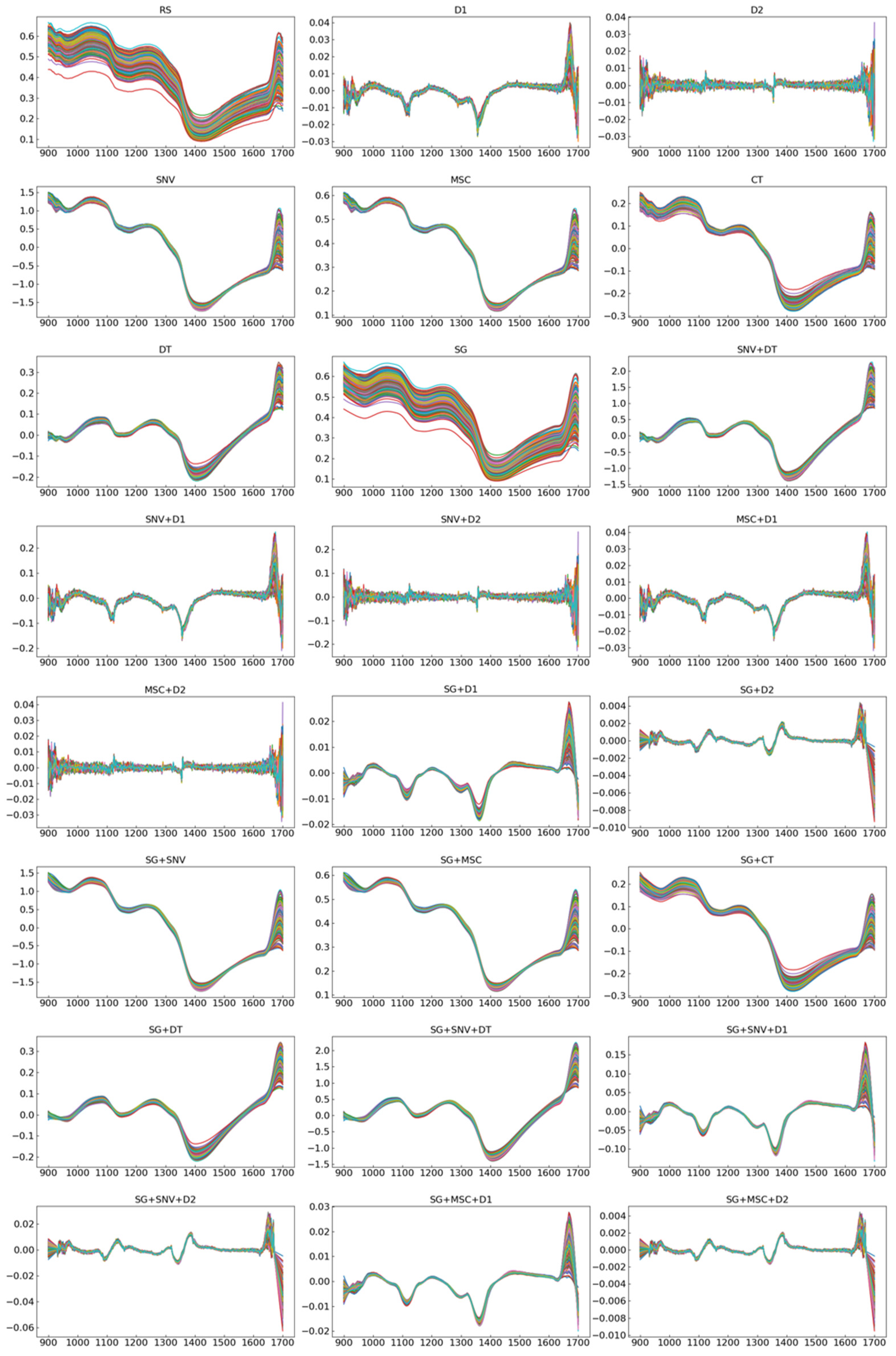
2.3. Pretreatment Transformations

The main pretreatment transformations of near-infrared spectroscopy include Savitzky–Golay (SG), first-order derivative (D1), second-order derivative (D2), standard normal variables (SNV), multiplicative scatter correction (MSC), mean center (CT), and shifted trend (DT) [18,19,21,22].
SG can remove the edge bands containing a considerable amount of noise from the spectrum profile by this procedure, improving the signal-to-noise ratio [23], enhancing the center wavelength point, and maximizing the retention of the peak features of the original spectral signal. D1 and D2 are able to eliminate the effect of linear baselines but enhance the noise to some level during processing. SNV and MSC remove the spectral disparities due to different scattering levels and enhance the spectral and data correlation [24,25]. Both CT and DT diminish the spectral shift. This experiment combined 24 pretreatment algorithms [26], as indicated in Table 1.

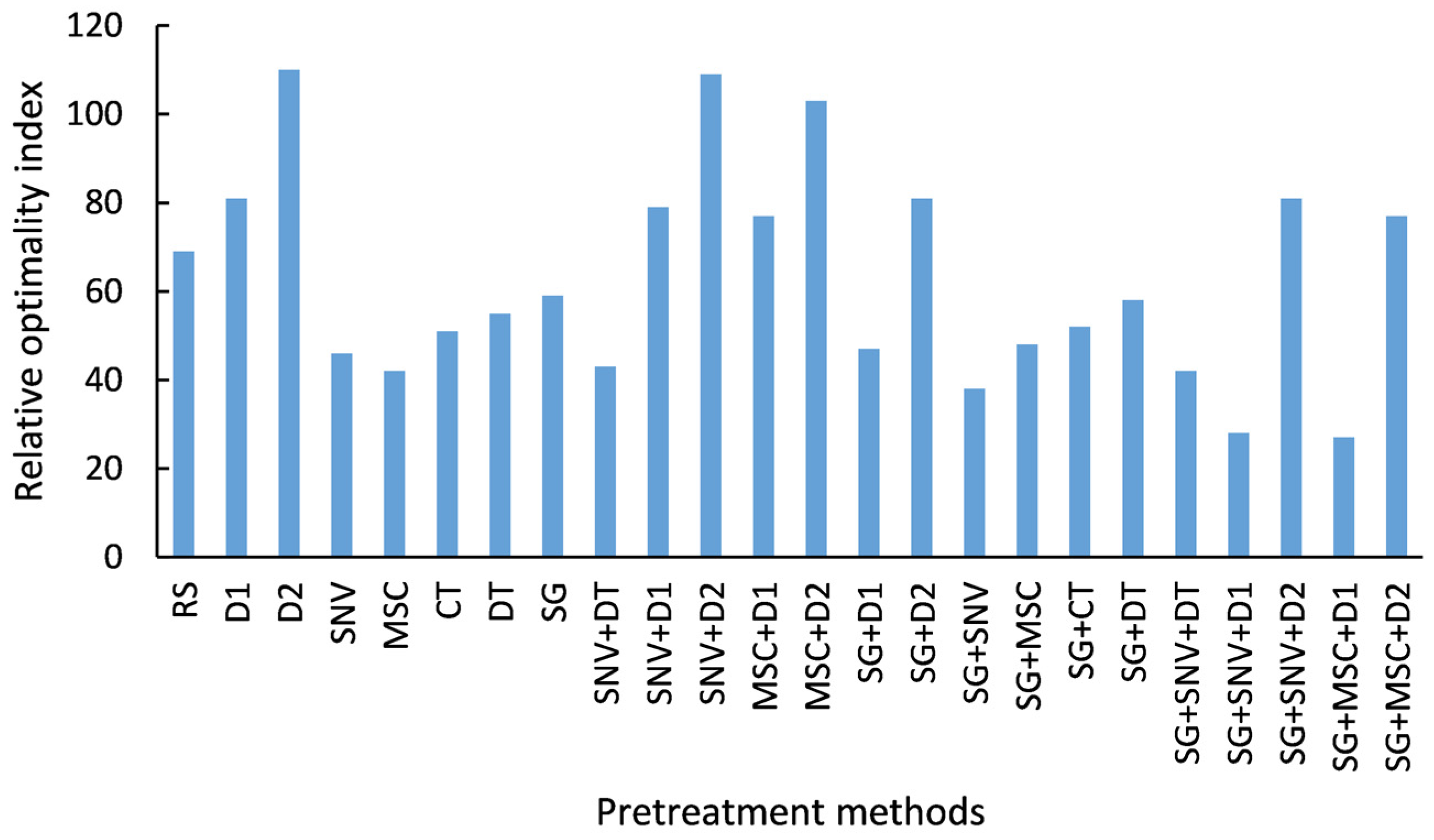
2.4. Ranking Method of Pretreatment Methods

In this paper, the impacts of 24 pretreatment methods on various models, such as random forest (RF), support vector machines (SVM), and boosting, were studied using NIR spectra. To select the optimal pretreatment method from the 24 pretreatment methods for identifying the woolliness response disease model of “Dangshan” pear, the relative optimality indexes of different pretreatment methods were calculated using Equation (2). The formula of the relative optimality index is provided in Equation (2).
R O I n d e x j = i = 1 n ( R A i j + R K i j )
In Equation (2), R O I n d e x j is the relative optimality index of pretreatment, and i and j represent the model type and pretreatment method, respectively. For model i , the accuracy of i under different pretreatment methods is calculated separately and ranked in descending order according to the numerical value, and the degree of influence of different pretreatment methods on the accuracy of i is distinguished by the accuracy list of i . R A i j denotes the accuracy of model i ranked in the accuracy list when the pretreatment method of the model is j . R K i j denotes the classification consistency level represented by the Kappa of model i when the pretreatment method is j . The R O I n d e x j of pretreatment method j is obtained by accumulating R A i j and R K i j under different models. R O I n d e x j takes into account the influence of different pretreatment methods on the model accuracy and classification consistency level and the effect of pretreatment methods on different models, which ensures the universality of pretreatment methods to some extent. Consequently, this experiment determined the optimal pretreatment method by comparing the R O I n d e x j of several pretreatment methods.

2.5. Classification Algorithms

To choose a suitable pretreatment method, three algorithms, RF, SVM, and boosting, which are more effective under traditional conditions, were chosen to model and analyse the data in this experiment to study the performance of near-infrared spectroscopy on DPWD under different pretreatment methods, comparing the ability of different models to handle DPWD under near-infrared spectroscopy.
Random forest is an ensemble-learning algorithm with a decision tree as the base learner, adding a layer of randomness to the bagging method. When making predictions, random forests will vote for the output result of all decision trees, finally selecting the class with the most votes as the output result of the random forest. This voting mechanism can reduce the error rate of individual decision trees and improve the accuracy of the entire model. In random forests, each node is partitioned using the best predictor in a randomly selected subset of predictors at that node. Its randomness allows random forests to demonstrate good power in classification problems and strong resilience to overfitting problems [27].
Support vector machine is a supervised machine learning method based on statistical learning theory and the structural risk minimization concept [28]. By producing a hyperplane, a nonlinear problem is transformed into a linear problem, a separation hyperplane is created between two points of different classes, and it is converted into a simple and manageable format [29]. This transformation of the data is achieved using a mathematical function known as the kernel function and is typically solved by SVM models with different kernel functions such as radial basis function (rbf), linear, sigmoid, polynomial (poly), etc. The sigmoid function is quite close to the rbf function [30]. The linear is a particular instance of rbf and is not necessary in the case of processing with rbf. In terms of accuracy, rbf has a greater interpolation capability than sigmoid, making the results of rbf more reliable. Consequently, rbf was chosen as the kernel function of SVM for modelling and analysis of NIR spectra in this experiment.
The ensemble model divided the collected data into a training set and a test set for training and evaluating weak classifiers and ensemble models. Data were used to train the selected weak classifiers and to construct the ensemble model using different methods. Ensemble learning methods were roughly categorized into boosting, bagging, and stacking. The boosting algorithm was an ensemble-learning method that improved the classification consistency by combining multiple weak classifiers into a single strong classifier [31]. Adaptive boosting (AdaBoost), gradient boosting decision tree (GBDT), and Xgboost are examples of boosting algorithms. AdaBoost is characterized by the fact that the weights of samples incorrectly classified by the previous basic classifier are increased, while the weights of samples well classified are reduced and used again to train the next basic classifier. AdaBoost is relatively sensitive to noise and outliers, as it pays more attention to misclassified samples in each iteration. GBDT produces a weak classifier in each iteration, and each classifier is trained on the residuals of the previous classifier. GBDT has a good ability to handle outliers and anomalies, but it cannot adaptively adjust sample weights. Xgboost performs a second-order Taylor expansion of the loss function in each learning round and adds a penalty term to prevent overfitting problems throughout the optimization process. Xgboost trains faster than GBDT, has higher accuracy, and can handle large-scale datasets.

2.6. Evaluation Metrics

In the evaluation of classification models, confusion matrices are generally used to evaluate binary classification models, which can be classified into four cases according to the difference between predicted and true results for a sample: true positive, false positive, true negative, and false negative, denoted by TP, FP, TN, and FN, respectively. To analyse the performance of different models more comprehensively and accurately, evaluation metrics such as accuracy, F1, and Kappa were used in this study to evaluate the performance of the models on the test set. The methods of calculating the relevant evaluation metrics are shown in the following equations.
A c c u r a c y = T P + T N T P + T N + F N + F P
F 1 = 2 T P 2 T P + F P + F N
K a p p a = P r ( a ) P r ( e ) 1 P r ( e )
P r ( a ) = T P + T N T P + T N + F N + F P
P r ( e ) = ( ( T P + F P ) × ( T P + F N ) n ) + ( ( F N + T N ) × ( T N + F P ) n ) n
Accuracy is the most basic evaluation metric when evaluating a model [32]. It evaluates the predictive ability of the model in terms of overall effectiveness but may give overly optimistic estimates due to the model’s dominance in overall classification while ignoring the prediction level of categories with smaller sample sets [33,34,35,36]. F1 is a metric used in statistics to quantify the accuracy of a dichotomous classification model, which considers both the accuracy and recall of the classification model. This article considered the importance of the model’s prediction abilities for different categories of samples and generated the F1 using the number of samples from different categories as weights. The kappa coefficient is a metric used to analyse the consistency in statistics and can be used to determine whether the anticipated and actual classification results of a classification model are consistent, taking values between (−1, 1). A higher Kappa suggests that the model achieved stronger classification consistency and fewer samples were misclassified. Table 2 demonstrates the level of classification consistency corresponding to Kappa at different intervals [37].

3. Results and Discussion

3.1. Dataset Statistics

A total of 480 samples of “Dangshan” pears were collected in this experiment, including 240 healthy samples and 240 sick samples. The 480 obtained samples were randomly assigned to the training set and the test set at a ratio of 7:3, of which the number of training sets was 336 and the number of test sets was 144. The data statistics of the training and test sets are provided in Table 3 below.
Pretreatment methods are an essential part of modelling analysis employing near-infrared spectroscopy, and the original spectral data can be purposely altered by different pretreatment methods. Figure 4 shows the NIR spectral images under 24 pretreatment methods, with the wavelength (nm) and absorbance (AU) of the spectra selected as the x-axis and y-axis of the images, respectively. Based on the RS images in Figure 4, it can be seen that the spectrum profiles of the 480 samples that underwent data collection by NIR techniques exhibited some resemblance in the overall trend, but they still had considerable variances. By comparing the spectral images under the original spectra and the other pretreatment methods, it can be seen that the D1 and D2-processed spectral images differed more from the original spectra; SG made the spectral curves smoother in general by removing the noise in the spectra; SNV and MSC had an effect on the range of values of the samples on different bands after scattering correction; DT created the original peaks in the spectra, but the original spectra peak became zero; and CT weakened the characteristic points of the spectrum while reducing the spectral offset.
To more intuitively compare the effects of different pretreatment methods on the sample data, the results under different pretreatment methods were processed using principal component analysis (PCA). PCA can reduce the dimensionality of the dataset and maximize the retention of original information while improving data interpretability [38] and is widely used in data downscaling and feature extraction [39]. PCA was able to reduce the number of original sample features to two, and the remaining two features were used as the horizontal and vertical axes to show the distribution of 480 samples on a two-dimensional plane. The distribution of samples under different pretreatments is shown in Figure 5, where H is the healthy sample and K is the diseased sample.
As shown in Figure 5, the sample point distributions of the healthy and diseased samples were concentrated, reflecting that the characteristics of the two samples possessed some similarity, which poses some difficulties for modelling and analysis using NIR analysis techniques. However, after transforming the original spectral data using different pretreatment methods, the point distribution of the 480 samples in the two-dimensional plane significantly changed. From the 24 two-dimensional distribution plots of the samples, we can see that SNV and MSC had a great similarity in their impact on near-infrared spectra, and there was a certain degree of substitutability between them. For example: SNV+D1 and MSC+D1; SG+ SNV and SG+MSC; SG+ SNV+D1 and SG+MSC+D1.

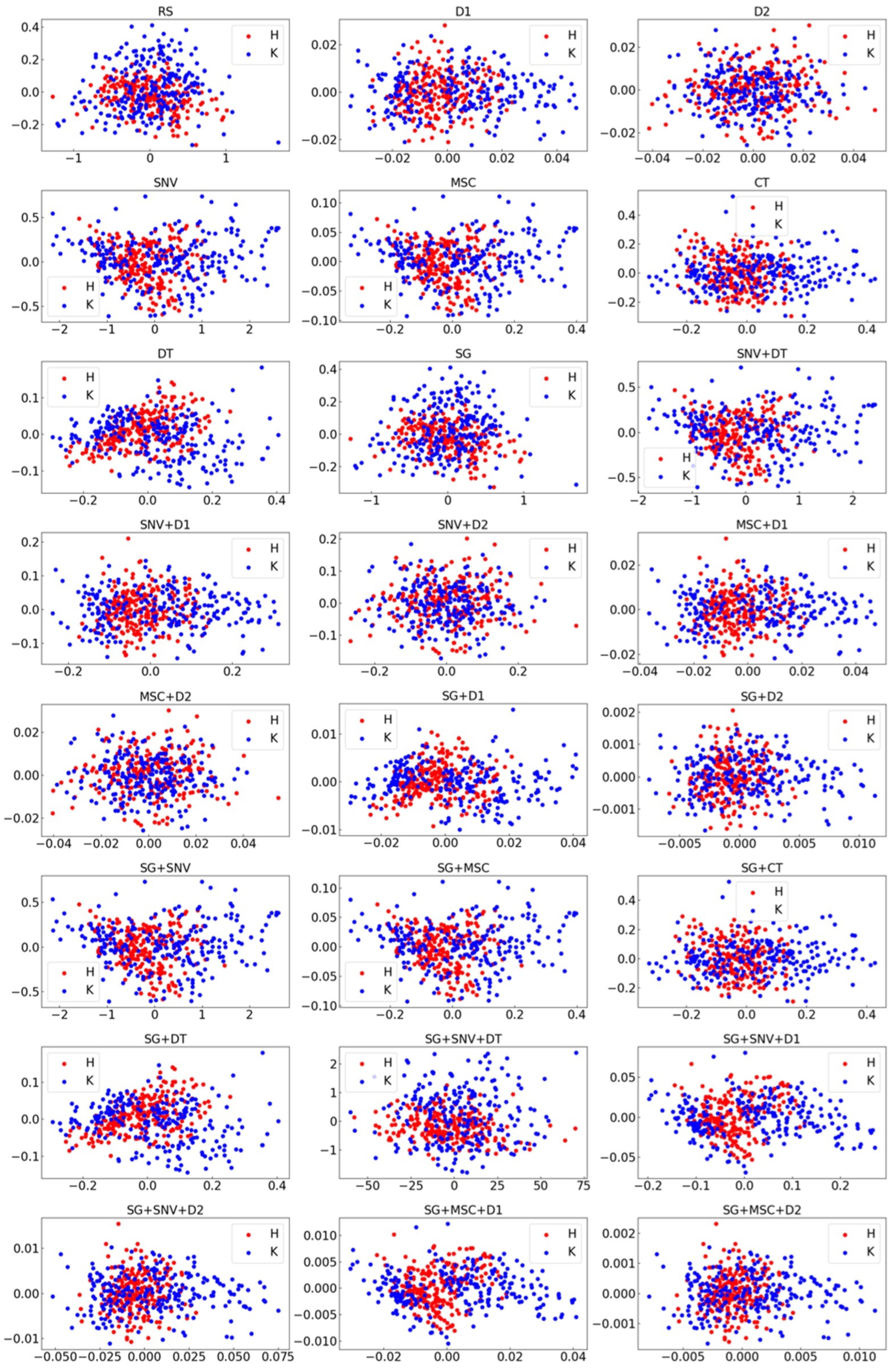
3.2. Analysis and Comparison of Optimal Pretreatment for “Dangshan” Pear Woolliness Disease Identification Modelling

To select the optimal pretreatment method, this study compared five kinds of classification algorithms under 24 kinds of near-infrared spectroscopy pretreatment methods, for a total of 120 classification models. Figure 6 shows the accuracy of SVM (rbf), RF and boosting models under 24 different pretreatment methods on the test set.
According to Figure 6, there were significant differences in the accuracy of the models under 24 different pretreatment methods. When the pretreatment methods were D2, SNV+D2, and MSC+D2, the accuracy of all five models was significantly lower than that of the models under RS. When the pretreatment methods were SG+SNV+D1 and SG+MSC+D1, the accuracies of the RF, AdaBoost, GBDT, and Xgboost models were all approximately 0.8, which was significantly improved compared with the accuracies of the models under RS. Hence, the choice of different pretreatment methods had a very close influence on the accuracy of the models. According to the performance of the accuracy of the five models under the 24 pretreatment methods, it can be seen that the degree of influence of the same pretreatment method on different models varied somewhat, which may improve the accuracy of some models while decreasing the accuracy of others. Considering the effects of 24 different pretreatment methods on the performance of different models, it was crucial to select the optimal pretreatment method for establishing the identification model of DPWD.
To select the optimal pretreatment method from 24 pretreatment methods, five models, including SVM, RF, AdaBoost, Xgboost, and GBDT, were experimentally selected to model and analyse the pretreatment raw spectral data, and the relative optimality index of each pretreatment method was calculated by Equation (2) based on the accuracy and Kappa of the five models under different pretreatment methods. By comparing the relative optimality index of different pretreatment methods, the pretreatment method with the lowest relative optimality index was selected as the optimal pretreatment method for this experiment. To evaluate the impact of different pretreatment methods on model performance, we arranged the performance of the same model under different pretreatment methods in descending order based on accuracy and calculated the classification consistency level corresponding to the model’s Kappa value. The results are shown in Table 4, where RA denotes the ranking of the impact of different pretreatment methods on the model’s accuracy and RK represents the Kappa-based classification consistency level of the model under different pretreatment methods.
According to Equation (2), the RA and RK of the five models under the pretreatment method were summed to obtain the ROIndex (relative optimality index) of this pretreatment method. The ROIndex of the 24 pretreatment methods are shown in Figure 7.
From Figure 7, it can be seen that among the 24 pretreatment methods, D1 and D2 had serious effects on the original spectral information, and the relative optimality index of D1, SNV+D1, MSC+D1, D2 and the pretreatment combinations including D2 were larger than those of RS. The relative optimality indexes of SG, SNV, and MSC were better than those of RS. Among all pretreatment methods, SG+SNV+D1 and the relative optimality index of SG+SNV+D1 and SG+MSC+D1 were the lowest among all pretreatment methods, 28 and 27, respectively, indicating that SG+SNV+D1 and SG+MSC+D1 were the optimal pretreatment methods for the DPWD identification model after analysing the effects of different pretreatment methods on the accuracy and Kappa of the five models.
Compared with RS, the performance of the models changed significantly when the pretreatment methods were SG+SNV+D1 and SG+MSC+D1, in which the accuracy and Kappa of the RF, AdaBoost, GBDT, and Xgboost models were significantly improved, but the performance of SVM did not change significantly, as shown in Table 5.

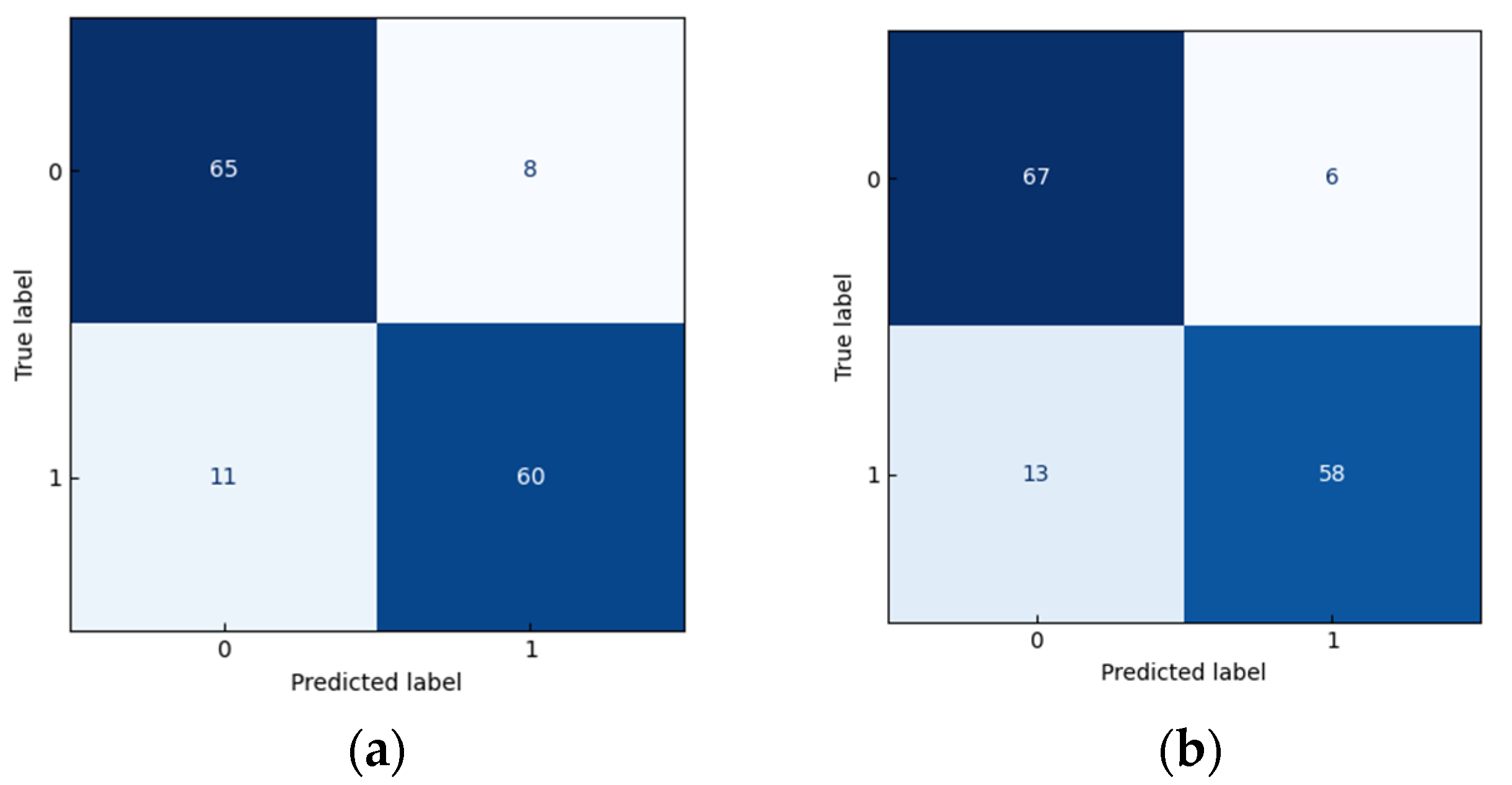
3.3. Optimization of the “Dangshan” Pear Woolliness Model on the Best Optimal Pretreatment Method

In the parameter debugging of SVM, the values of three parameters, such as the kernel function (Kernel), penalty factor (PT), and gamma, are selected according to the magnitude of the accuracy of different models, and the values of the three parameters in the model with the highest accuracy are used as the results of parameter debugging. The kernel function is a way for SVM models to map the input variables to a high-dimensional feature space, and the common kernel functions are the linear kernel function (linear), polynomial kernel function (poly), sigmoid function (sigmoid), and radial basis function (RBF). PT is a penalty factor of SVM to balance the weight of classification intervals and misclassification points. The larger the PT is, the higher the cost of misclassification and the less likely the model will be overfitted. If the PT is too small, the SVM will prefer to select larger intervals, which may lead to overfitting. Therefore, it is important to choose an appropriate PT value to balance the complexity and generalization ability of the model. The gamma parameter in SVM affects the decision boundary. A low gamma will result in a wider decision boundary, while a high gamma will result in a more complex decision boundary that may overfit the data.
Both RF and boosting models choose the maximum depth of the decision tree (max_depth) and the maximum number of iterations of the weak learner (max_NIO) as the debugging objects. max_depth is the maximum depth of each weak learner, which can limit the number of nodes in the classification tree. A small value of max_NIO leads to a simpler structure of the trained model, which cannot make accurate predictions for the samples in the training and test sets. When max_NIO is too large, the model lacks generalization ability and cannot effectively predict the untrained samples. In addition to debugging max_depth and max_NIO, RF will also select the classification criteria for decision tree nodes and compare the impact of the two criteria for classifying decision tree nodes, gini and entropy, on the model.
In the parameter debugging process, the parameter ranges and step sizes for different models are shown in Table 6.
In the process of parameter debugging, the SVM selects rbf, linear, poly, and sigmoid as kernel functions in turn, and the PT and Gamma of the model are selected under the selected kernel functions. When other parameters remain unchanged, PT increases from 1 according to the step size within the value range of PT, and the PT with the highest accuracy is selected according to the model accuracy under different PT conditions. In the case of determining the values of Kernel and PT, the value of Gamma that makes the highest accuracy of the model in three ranges is selected, and the values of Kernel, PT, and Gamma are taken as the results of SVM parameter debugging.
In the parameter debugging of RF, gini and entropy are selected as the classification criteria of classification tree nodes in turn, and the values of max_depth and max_NIO are determined under the selected criteria. When the other parameters remain unchanged, max_depth is increased in steps from 1 in the range of values, and the value of max_depth is selected as the optimal value of max_depth when RF has the highest accuracy. In the case of determining the classification criterion and max_depth of the classification tree, the value of max_NIO that makes the highest accuracy of RF is selected, and the values of Criterion, max_depth, and max_NIO are taken as the results of parameter debugging of RF.
In the parameter debugging of AdaBoost, GBDT, and Xgboost, the values of max_depth and max_NIO are selected successively within the range of parameter values while keeping other parameters unchanged. In the process of determining max_depth, max_depth is increased in steps from 1 in the range of values, and the value of max_depth that makes the model most accurate is selected as the optimal value of max_depth. Under the optimal max_depth, the value of max_NIO that makes the highest accuracy of the model is selected as the optimal value of max_NIO, and the optimal values of max_depth and max_NIO are used as the parameter debugging results of boosting models.
The accuracy and Kappa of different models after parameter debugging under the best pretreatment methods are shown in Table 7.
According to the information in Table 7, the accuracy of different models was significantly improved after pretreatment and parameter debugging, and the accuracy of five models, SVM, RF, AdaBoost, GBDT, and Xgboost, was approximately 0.85 after pretreatment and parameter debugging, among which SVM after SG+SNV+D1 processing and AdaBoost after SG+MSC+D1 processing were the optimal models for this experiment.
To show the prediction ability of the model for different categories of samples more visually, the confusion matrix was used to further demonstrate the classification of SVM and AdaBoost, and the confusion matrix of the two models is shown in Figure 8.
In Figure 8, SVM and AdaBoost predicted 144 samples, SVM successfully predicted 125 samples, misclassified 11 diseased and 8 healthy samples, and AdaBoost successfully predicted 125 samples, misclassified 13 diseased and 6 healthy samples. Although there were some differences in model accuracy between SVM and AdaBoost in predicting different classes of samples, both models showed good predictive ability, demonstrating the feasibility of using near-infrared analysis technology to identify DPWD.
Based on different usage scenarios, the members of our team used different methods to establish recognition models for the DPWD. In Yuanfeng Chen’s research, the improvement of model performance was emphasized by fusing near-infrared spectroscopy and neural network features based on images by comparing the changes in model accuracy before and after data fusion. Finally, in all the results, the accuracy of the optimal model after feature fusion was 0.9722. In Yuanfeng Chen’s research, pretreatment methods were not used to optimize the spectral data when establishing a model. When only near-infrared spectroscopy was used for modelling, the accuracy rates were all below 0.62, indicating poor performance of the models. This article established a classification model for DPWP using near-infrared technology. It focused on discussing the importance of pretreatment methods in improving the predictive ability of the model and defined a new measurement method to evaluate the impact of different pretreatment methods on model performance. Ultimately, under the optimal pretreatment method, the accuracy of the optimal model in this study was 0.87.
This article discussed the impact of pretreatment methods and model types on the predictive power of models, using near-infrared technology to establish a stable identification model under restricted conditions. However, the accuracy of the model was still far from the research of Yuanfeng Chen. Based on the information in Figure 8, it can be found that the probability of the model making errors when predicting diseased samples was higher than the probability of making errors when predicting healthy samples. This difference may be because the model needs a larger training set to improve its ability to recognize diseased samples. Therefore, in further improving the model process, attempts will be made to increase the sample size of the training set to further study the accuracy of the model. When team member Lianglong Wang used near-infrared technology to predict the nutrition deficiency of fresh pear leaves, the appropriate feature extraction method had a positive impact on improving the accuracy of the model. Therefore, it is also possible to consider introducing feature extraction methods to further improve the performance of the model.

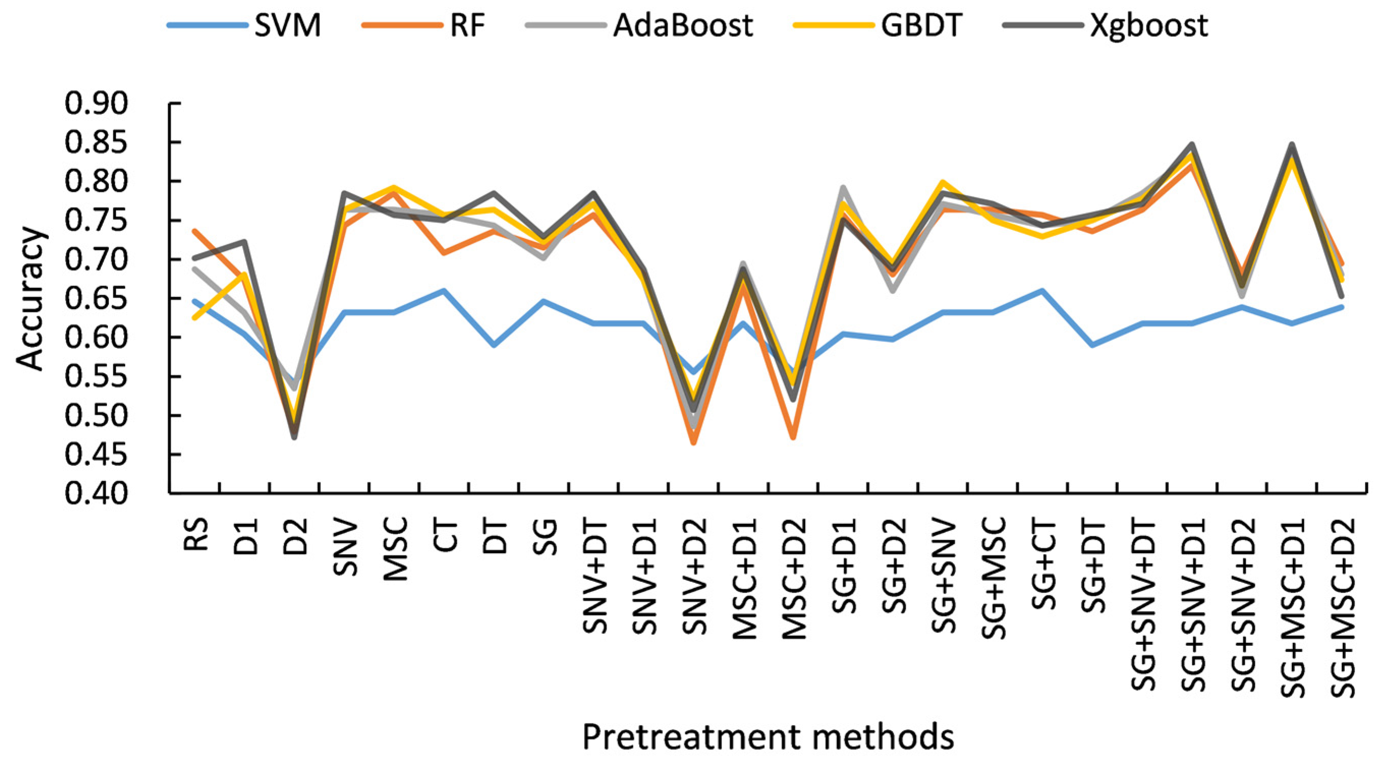
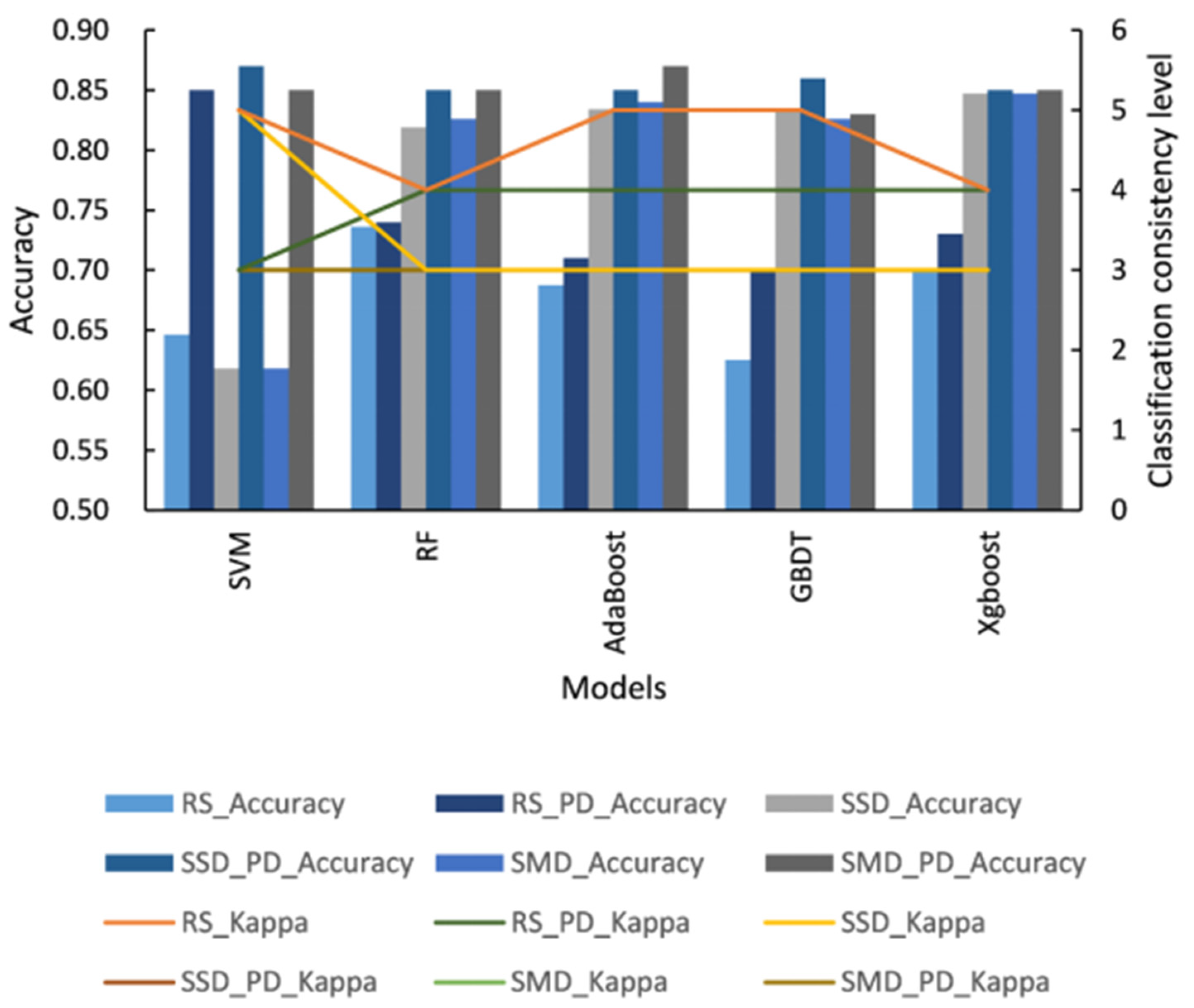
3.4. The Effect of Parameter Debugging and Pretreatment Methods on the Performance of Different Models

In this experiment, all five models showed excellent classification ability under the combined effect of optimal pretreatment and parameter debugging, but the reaction of different models to pretreatment and parameter debugging varied significantly. To further understand the effects of pretreatment and parameter debugging on different models, Figure 9 shows the accuracy and classification consistency levels of different models before and after parameter debugging. In Figure 9, the different characters have the following meanings: “RS”, “SSD”, and “SMD” indicate that the model was preprocessed as RS, SG+SNV+D1, and SG+MSC+D1, respectively; “PD” indicates that the model was parameter debugged; “Accuracy” and “Kappa” represent the accuracy and classification consistency of the model, respectively. For example, “SSD_PD_Accuracy” refers to the accuracy of the model after parameter debugging when the pretreatment method was SG+SNV+D1, and “SSD_PD_Kappa” refers to the classification consistency level of the model after parameter debugging when the pretreatment method was SG+SNV+D1.
According to Figure 9, it can be seen that the SVM and boosting models had significantly different requirements for pretreatment methods, and the pretreatment methods had a more pronounced effect on the RF and boosting models. Under the optimal pretreatment, the accuracy and classification consistency levels of RF and boosting were significantly improved, where the accuracy ratios rose from 0.74 (RF), 0.69 (AdaBoost), 0.63 (GBDT), and 0.70 (Xgboost) to between 0.8 and 0.85, respectively, and the classification consistency level rose from 3 to 5. The classification consistency increased by two levels, and the overall performance of the model was close to that of the parameter-debugged model. Consequently, the pretreatment method had an important impact on the performance of RF and boosting. Under the optimal pretreatment, the accuracy of SVM decreased to some extent, compared with that before preprocessing, but the accuracy of the model after parameter debugging increased from approximately 0.6 to approximately 0.8, the classification consistency level increased to level 3, and the performance of the model improved significantly. To compare the effects of pretreatment methods and parameter debugging on SVM, the parameters of SVM were debugged under three different pretreatment methods, RS, SG+SNV+D1, and SG+MSC+D1, and the final results showed that the accuracy of the SVM model after parameter debugging under different pretreatment methods was significantly improved. Therefore, compared with SVM, ensemble learning models such as RF and boosting were more sensitive to pretreatment methods and can reflect better model performance with appropriate pretreatment methods, while the performance of SVM was more dependent on the internal parameters of the model lazily, and the pretreatment methods had less influence on the performance of SVM.
The SVM’s sensitivity to pretreatment methods can be indirectly confirmed from the information shown in Figure 5. In Figure 5, there was no significant difference in the distribution of the healthy and diseased samples under different pretreatment methods. Therefore, during the process of SVM correctly classifying the training dataset and finding the separation hyperplane with the maximum geometrical margin, the different pretreatment methods had a minor impact on the results. RF and boosting models were better-performing classifiers obtained by integrating and selecting weak classifiers. The quality of data directly affected the effectiveness of the classifier. After appropriate pretreatment and transformation, problems such as scattering, baseline variations, peak shifts, noise, missing values, and other issues in the data were weakened to a certain extent. These pretreatment methods can further extract the real information contained in the data, making it more meaningful. Therefore, RF and boosting algorithms require appropriate pretreatment methods to be better applied in data analysis.

4. Conclusions

In this paper, 24 pretreatment methods were analysed using the original spectral reflectance dataset and 120 classification models. The results of the study are summarized as follows:
  • After processing the spectral data with suitable pretreatment methods, SVM and AdaBoost based on NIR spectra had excellent performance in terms of accuracy, F1, and Kappa after parameter debugging, which proves the feasibility of near-infrared spectroscopy in identifying the woolliness response disease of “Dangshan” pear.
  • The influence of different pretreatment methods on the modelling analysis using near-infrared spectroscopy was different. D2 had a severe influence on the original spectra, and different models showed lower prediction ability in the identification of “Dangshan” pear woolliness response disease with D2 or pretreatment methods including D2. SG+SNV+D1 and SG+MSC+D1 were the two best pretreatment methods in this experiment and played an important role in the identification of woolliness response disease of “Dangshan” pear using near-infrared spectroscopy.
  • Models such as RF, AdaBoost, GBDT, and Xgboost were more stringent for the pretreatment methods in identifying the woolliness response disease of “Dangshan” pear, and the performance of the models was significantly improved with a suitable pretreatment method.
This paper demonstrated that near-infrared spectroscopy can accurately and quickly detect DPWD, providing a new method for the detection of DPWD in agricultural production. To further improve the performance of the enhanced prediction model and reduce the probability of misclassifying the samples, the model will be further improved using different feature extraction methods to provide a more reliable reference for actual agricultural production.

Author Contributions

Data curation, J.Z. and X.J.; formal analysis, J.Z. and X.J.; investigation, L.L.; methodology, X.J. and Y.C.; project administration, L.L.; resources, Y.R. and X.Z.; supervision, X.J. and Y.C.; validation, X.J.; writing—original draft preparation, J.Z.; writing—review and editing, X.J. All authors have read and agreed to the published version of the manuscript.

Funding

This study was supported by Key Research and Development Project of Anhui Province in 2022 (Project No: 202204c06020022), Key Research, Development Project of Anhui Province in 2022 (Project No: 202204c06020022), and Anhui Province Major Research Project (Project No: 2022AH040125).

Data Availability Statement

The datasets generated for this study are available on request to the corresponding author.

Conflicts of Interest

The authors declare no conflict of interest.

References

  1. Silva, G.J.; Souza, T.M.; Barbieri, R.L.; Costa de Oliveira, A. Origin, Domestication, and Dispersing of Pear (Pyrus Spp.). Adv. Agric. 2014, 2014, 541097. [Google Scholar] [CrossRef]
  2. Zeng, W.; Qiao, X.; Li, Q.; Liu, C.; Wu, J.; Yin, H.; Zhang, S. Genome-Wide Identification and Comparative Analysis of the ADH Gene Family in Chinese White Pear (Pyrus Bretschneideri) and Other Rosaceae Species. Genomics 2020, 112, 3484–3496. [Google Scholar] [CrossRef] [PubMed]
  3. Li, X.; Zhang, J.; Gao, W.; Wang, H. Study on Chemical Composition, Anti-Inflammatory and Anti-Microbial Activities of Extracts from Chinese Pear Fruit (Pyrus Bretschneideri Rehd.). Food Chem. Toxicol. 2012, 50, 3673–3679. [Google Scholar] [CrossRef] [PubMed]
  4. Li, X.; Wang, T.; Zhou, B.; Gao, W.; Cao, J.; Huang, L. Chemical Composition and Antioxidant and Anti-Inflammatory Potential of Peels and Flesh from 10 Different Pear Varieties (Pyrus Spp.). Food Chem. 2014, 152, 531–538. [Google Scholar] [CrossRef] [PubMed]
  5. Chen, J.; Wang, Z.; Wu, J.; Wang, Q.; Hu, X. Chemical Compositional Characterization of Eight Pear Cultivars Grown in China. Food Chem. 2007, 104, 268–275. [Google Scholar] [CrossRef]
  6. Haifa, P.; Yiliu, X.; Yi, Z.; Jinyun, Z.; Zhenghui, G.; Xingkai, Y. Effects of Boron on the Growth and Fruit Quality of Dangshansu Pear(Pyrus Bretshneideri Cv.Dangshansu Pear). Plant Nutr. Fertil. Sci. 2011, 17, 1024–1029. [Google Scholar]
  7. González-Agüero, M.; Pavez, L.; Ibáñez, F.; Pacheco, I.; Campos-Vargas, R.; Meisel, L.A.; Orellana, A.; Retamales, J.; Silva, H.; González, M.; et al. Identification of Woolliness Response Genes in Peach Fruit after Post-Harvest Treatments. J. Exp. Bot. 2008, 59, 1973–1986. [Google Scholar] [CrossRef]
  8. Cortés, V.; Blasco, J.; Aleixos, N.; Cubero, S.; Talens, P. Visible and Near-Infrared Diffuse Reflectance Spectroscopy for Fast Qualitative and Quantitative Assessment of Nectarine Quality. Food Bioprocess Technol. 2017, 10, 1755–1766. [Google Scholar] [CrossRef]
  9. Cocchi, M.; Corbellini, M.; Foca, G.; Lucisano, M.; Pagani, M.A.; Tassi, L.; Ulrici, A. Classification of Bread Wheat Flours in Different Quality Categories by a Wavelet-Based Feature Selection/Classification Algorithm on NIR Spectra. Anal. Chim. Acta 2005, 544, 100–107. [Google Scholar] [CrossRef]
  10. Miralbés, C. Discrimination of European Wheat Varieties Using near Infrared Reflectance Spectroscopy. Food Chem. 2008, 106, 386–389. [Google Scholar] [CrossRef]
  11. Jin, X.; Ba, W.; Wang, L.; Zhang, T.; Zhang, X.; Li, S.; Rao, Y.; Liu, L. A Novel Tran_NAS Method for the Identification of Fe- and Mg-Deficient Pear Leaves from N- and P-Deficient Pear Leaf Data. ACS Omega 2022, 7, 39727–39741. [Google Scholar] [CrossRef]
  12. Jin, X.; Wang, L.; Zheng, W.; Zhang, X.; Liu, L.; Li, S.; Rao, Y.; Xuan, J. Predicting the Nutrition Deficiency of Fresh Pear Leaves with a Miniature Near-Infrared Spectrometer in the Laboratory. Measurement 2022, 188, 110553. [Google Scholar] [CrossRef]
  13. Ba, W.; Jin, X.; Lu, J.; Rao, Y.; Zhang, T.; Zhang, X.; Zhou, J.; Li, S. Research on Predicting Early Fusarium Head Blight with Asymptomatic Wheat Grains by Micro-near Infrared Spectrometer. Spectrochim. Acta A Mol. Biomol. Spectrosc. 2023, 287, 122047. [Google Scholar] [CrossRef]
  14. Shao, X.; Ning, Y.; Liu, F.; Li, J.; Cai, W. Application of Near-Infrared Spectroscopy in Micro Inorganic Analysis. Acta Chim. Sin. 2012, 70, 2109. [Google Scholar] [CrossRef]
  15. Mishra, P.; Biancolillo, A.; Roger, J.M.; Marini, F.; Rutledge, D.N. New Data Preprocessing Trends Based on Ensemble of Multiple Preprocessing Techniques. TrAC Trends Anal. Chem. 2020, 132, 116045. [Google Scholar] [CrossRef]
  16. Engel, J.; Gerretzen, J.; Szymańska, E.; Jansen, J.J.; Downey, G.; Blanchet, L.; Buydens, L.M.C. Breaking with Trends in Pre-Processing? TrAC Trends Anal. Chem. 2013, 50, 96–106. [Google Scholar] [CrossRef]
  17. Oliveri, P.; Malegori, C.; Simonetti, R.; Casale, M. The Impact of Signal Pre-Processing on the Final Interpretation of Analytical Outcomes—A Tutorial. Anal. Chim. Acta 2019, 1058, 9–17. Available online: https://www.semanticscholar.org/paper/The-impact-of-signal-pre-processing-on-the-final-of-Oliveri-Malegori/513c8c6936c5e566f0d2f8c378cddb15f54acf26 (accessed on 7 March 2023). [CrossRef] [PubMed]
  18. Gerretzen, J.; Szymańska, E.; Jansen, J.J.; Bart, J.; van Manen, H.-J.; van den Heuvel, E.R.; Buydens, L.M.C. Simple and Effective Way for Data Preprocessing Selection Based on Design of Experiments. Anal. Chem. 2015, 87, 12096–12103. [Google Scholar] [CrossRef]
  19. Bian, X.; Wang, K.; Tan, E.; Diwu, P.; Zhang, F.; Guo, Y. A Selective Ensemble Preprocessing Strategy for Near-Infrared Spectral Quantitative Analysis of Complex Samples. Chemom. Intell. Lab. Syst. 2020, 197, 103916. [Google Scholar] [CrossRef]
  20. Chen, Y.; Liu, L.; Rao, Y.; Zhang, X.; Zhang, W.; Jin, X. Identifying the “Dangshan” Physiological Disease of Pear Woolliness Response via Feature-Level Fusion of Near-Infrared Spectroscopy and Visual RGB Image. Foods 2023, 12, 1178. [Google Scholar] [CrossRef]
  21. Roger, J.-M.; Biancolillo, A.; Marini, F. Sequential Preprocessing through ORThogonalization (SPORT) and Its Application to near Infrared Spectroscopy. Chemom. Intell. Lab. Syst. 2020, 199, 103975. [Google Scholar] [CrossRef]
  22. Mishra, P.; Roger, J.M.; Rutledge, D.N.; Woltering, E. SPORT Pre-Processing Can Improve Near-Infrared Quality Prediction Models for Fresh Fruits and Agro-Materials. Postharvest Biol. Technol. 2020, 168, 111271. [Google Scholar] [CrossRef]
  23. Shi, X.; Yao, L.; Pan, T. Visible and Near-Infrared Spectroscopy with Multi-Parameters Optimization of Savitzky-Golay Smoothing Applied to Rapid Analysis of Soil Cr Content of Pearl River Delta. GEP 2021, 09, 75–83. [Google Scholar] [CrossRef]
  24. Barnes, R.J.; Dhanoa, M.S.; Lister, S.J. Standard Normal Variate Transformation and De-Trending of Near-Infrared Diffuse Reflectance Spectra. Appl. Spectrosc. 1989, 43, 772–777. [Google Scholar] [CrossRef]
  25. Isaksson, T.; Næs, T. The Effect of Multiplicative Scatter Correction (MSC) and Linearity Improvement in NIR Spectroscopy. Appl. Spectrosc. 1988, 42, 1273–1284. [Google Scholar] [CrossRef]
  26. Jin, X.; Li, S.; Zhang, W.; Zhu, J.; Sun, J. Prediction of Soil-Available Potassium Content with Visible Near-Infrared Ray Spectroscopy of Different Pretreatment Transformations by the Boosting Algorithms. Appl. Sci. 2020, 10, 1520. [Google Scholar] [CrossRef]
  27. Liaw, A.; Wiener, M. Classification and Regression by randomForest. R News 2002, 2, 18–22. [Google Scholar]
  28. Tien Bui, D.; Pradhan, B.; Lofman, O.; Revhaug, I. Landslide Susceptibility Assessment in Vietnam Using Support Vector Machines, Decision Tree, and Naïve Bayes Models. Math. Probl. Eng. 2012, 2012, 974638. [Google Scholar] [CrossRef]
  29. Jebur, M.N.; Pradhan, B.; Tehrany, M.S. Optimization of Landslide Conditioning Factors Using Very High-Resolution Airborne Laser Scanning (LiDAR) Data at Catchment Scale. Remote Sens. Environ. 2014, 152, 150–165. [Google Scholar] [CrossRef]
  30. Song, S.; Zhan, Z.; Long, Z.; Zhang, J.; Yao, L. Comparative Study of SVM Methods Combined with Voxel Selection for Object Category Classification on FMRI Data. PLoS ONE 2011, 6, e17191. [Google Scholar] [CrossRef]
  31. Schapire, R.E. Explaining AdaBoost; Schölkopf, B., Luo, Z., Vovk, V., Eds.; Springer: Berlin/Heidelberg, Germany, 2013; pp. 37–52. [Google Scholar]
  32. Wang, L.; Chu, F.; Xie, W. Accurate Cancer Classification Using Expressions of Very Few Genes. IEEE/ACM Trans. Comput. Biol. Bioinf. 2007, 4, 40–53. [Google Scholar] [CrossRef]
  33. Sokolova, M.; Japkowicz, N.; Szpakowicz, S. Beyond Accuracy, F-Score and ROC: A Family of Discriminant Measures for Performance Evaluation. In Advances in Artificial Intelligence; Springer: Berlin/Heidelberg, Germany, 2006; Available online: https://link.springer.com/chapter/10.1007/11941439_114 (accessed on 16 March 2023).
  34. Gu, Q.; Zhu, L.; Cai, Z. Evaluation Measures of the Classification Performance of Imbalanced Data Sets. In Computational Intelligence and Intelligent Systems. ISICA 2009; Springer: Berlin/Heidelberg, Germany, 2009; Available online: https://link.springer.com/chapter/10.1007/978-3-642-04962-0_53 (accessed on 16 March 2023).
  35. Bekkar, M.; Djemaa, H.; Alitouche, T.A. Evaluation Measures for Models Assessment over Imbalanced Data Sets. J. Inf. Eng. Appl. 2013, 3, 27–38. [Google Scholar]
  36. Akosa, J. Predictive Accuracy: A Misleading Performance Measure for Highly Imbalanced Data. Proc. SAS Glob. Forum 2017, 12, 1–4. [Google Scholar]
  37. McHugh, M.L. Interrater Reliability: The Kappa Statistic. Biochem. Med. 2012, 276–282. [Google Scholar] [CrossRef]
  38. Jolliffe, I.T.; Cadima, J. Principal Component Analysis: A Review and Recent Developments. Phil. Trans. R. Soc. A 2016, 374, 20150202. [Google Scholar] [CrossRef] [PubMed]
  39. Uddin, P.; Mamun, A.; Hossain, A. PCA-Based Feature Reduction for Hyperspectral Remote Sensing Image Classification. IETE Tech. Rev. 2021, 38, 377–396. [Google Scholar] [CrossRef]
Figure 1. Comparative views of healthy and diseased samples: (a) surface view of a healthy sample; (b) surface view of a diseased sample; (c) profile view of the healthy sample; (d) profile view of the diseased sample.
Agronomy 13 01420 g001aAgronomy 13 01420 g001b
Figure 2. “NIR-S-G1” miniature spectral acquisition apparatus.
Agronomy 13 01420 g002
Figure 3. Five-point sampling map of the “Dangshan” pear.
Agronomy 13 01420 g003
Figure 4. NIR spectra with different pretreatment transformations.
Agronomy 13 01420 g004
Figure 5. Two-dimensional visualization of spectra under different pretreatment methods.
Agronomy 13 01420 g005
Figure 6. Accuracy of the model on the test set under different pretreatment methods.
Agronomy 13 01420 g006
Figure 7. Relative optimality index of the pretreatment method.
Agronomy 13 01420 g007
Figure 8. Confusion matrix of the optimal model: (a) SVM under the SG+SNV+D1 pretreatment method; (b) AdaBoost under the SG+MSC+D1 pretreatment method.
Agronomy 13 01420 g008
Figure 9. Analysis of accuracy and classification consistency with parameter debugging and different pretreatments.
Agronomy 13 01420 g009
Table 1. Pretreatment methods applied to the near-infrared spectroscopy of “Dangshan” pear.
Pretreatment MethodAbbreviations
Reflection spectrum without pretreatment methodRS
First derivativeD1
Second derivativeD2
Standard normal variateSNV
Multiplicative scatter correctionMSC
Mean centerCT
Dislodge tendencyDT
Savitzky–GolaySG
Dislodge tendency with standard normal variateSNV + DT
First derivative with standard normal variateSNV + D1
Second derivative with standard normal variateSNV + D2
First derivative with multiplicative scatter correctionMSC + D1
Second derivative with multiplicative scatter correctionMSC + D2
First derivative with Savitzky–GolaySG + D1
Second derivative with Savitzky–GolaySG + D2
Standard normal variate with Savitzky–GolaySG + SNV
Multiplicative scatter correction with Savitzky–GolaySG + MSC
Mean center with Savitzky–GolaySG + CT
Dislodge tendency with Savitzky–GolaySG + DT
Dislodge tendency with standard normal variate and Savitzky–GolaySG + SNV + DT
First derivative with standard normal variate and Savitzky–GolaySG + SNV + D1
Second derivative with standard normal variate and Savitzky–GolaySG + SNV + D2
First derivative with multiplicative scatter correction and Savitzky–GolaySG + MSC + D1
Second derivative with multiplicative scatter correction and Savitzky–GolaySG + MSC + D2
Table 2. Classification consistency levels corresponding to Kappa.
Numerical Range (Kappa)Classification ConsistencyClassification Consistency Levels
<0Totally Inconsistent7
0.0–0.20None6
0.21–0.39Minimal5
0.40–0.59Weak4
0.60–0.79Moderate3
0.80–0.90Strong2
Above 0.90Almost Perfect1
Table 3. Pear sample statistics.
TypeTotal NumberNumber of DiseasedNumber of Healthy
Total number of samples480240240
Training set336169167
Test set1447173
Table 4. Accuracy and classification consistency of the model with different pretreatment methods.
Pretreatment
Method
SVMRFAdaBoostGBDTXgboost
RARKRARKRARKRARKRARK
RS257412516594
D16612517513584
D2106147196197157
SNV4564647424
MSC4534644444
CT1594748454
DT8674947424
SG258410411474
SNV+DT5554446424
SNV+D155115145145105
SNV+D296167207186146
MSC+D155135115135105
MSC+D296157186176136
SG+D16654346454
SG+D276115155125105
SG+SNV4544543324
SG+MSC4544749434
SG+CT15549410464
SG+DT8674849444
SG+SNV+DT5544445434
SG+SNV+D15523231313
SG+SNV+D235115165155115
SG+MSC+D15513132313
SG+MSC+D235105135145125
Table 5. Accuracy and Kappa of the model under the optimal pretreatment method.
Pretreatment
Method
RSSG+SNV+D1SG+MSC+D1
AccuracyKappaAccuracyKappaAccuracyKappa
SVM0.650.290.620.230.620.23
RF0.740.470.820.640.830.67
AdaBoost0.690.360.830.670.840.68
GBDT0.630.250.830.670.830.65
Xgboost0.700.400.850.690.850.69
Table 6. Parameters to be debugged by the model in the parameter debugging process.
ModelParametersValue Range and Step Size
SVMKernelrbf, poly, linear, sigmoid
PT(1, 2000, 50)
Gamma(0.01, 1, 0.01)
(1, 50, 1)
(1, 1500, 50)
RFCriteriongini, entropy
max_depth(1, 30, 1)
max_NIO(1, 1500, 50)
Xgboostmax_depth(1, 30, 1)
max_NIO(1, 1500, 50)
AdaBoostmax_depth(1, 30, 1)
max_NIO(1, 1500, 50)
GBDTmax_depth(1, 30, 1)
max_NIO(1, 1500, 50)
Table 7. Accuracy and Kappa of the model after the selection of parameters.
Pretreatment
Method
SG+SNV+D1SG+MSC+D1
ParameterAccuracyF1KappaParameterAccuracyF1Kappa
SVMKernel = rbf0.870.870.74Kernel = rbf0.850.850.71
PT = 701PT = 701
Gamma = 32Gamma = 701
RFCriterion = gini0.850.850.69Criterion = gini0.850.850.69
max_depth = 12max_depth = 12
max_NIO = 201max_NIO = 651
AdaBoostmax_depth = 20.850.850.71max_depth = 30.870.870.74
max_NIO = 251max_NIO = 101
GBDTmax_depth = 30.860.860.72max_depth = 30.830.830.65
max_NIO = 601max_NIO = 1451
Xgboostmax_depth = 60.850.850.69max_depth = 60.850.850.71
max_NIO = 101max_NIO = 501
Disclaimer/Publisher’s Note: The statements, opinions and data contained in all publications are solely those of the individual author(s) and contributor(s) and not of MDPI and/or the editor(s). MDPI and/or the editor(s) disclaim responsibility for any injury to people or property resulting from any ideas, methods, instructions or products referred to in the content.

