Article

Hyperspectral Technique for Detection of Peanut Leaf Spot Disease Based on Improved PCA Loading

1
College of Information and Electrical Engineering, Shenyang Agricultural University, Shenyang 110866, China
2
College of Computer Science and Technology, Inner Mongolia University for Nationalities, Tongliao 028000, China
3
School of Information Science and Engineering, Shenyang Ligong University, Shenyang 110866, China
*
Author to whom correspondence should be addressed.
Agronomy 2023, 13(4), 1153; https://doi.org/10.3390/agronomy13041153
Submission received: 17 March 2023 / Revised: 10 April 2023 / Accepted: 16 April 2023 / Published: 18 April 2023
(This article belongs to the Special Issue The Application of Near-Infrared Spectroscopy in Agriculture)

Abstract

:
Leaf spot disease is a dangerous disease that affects peanut growth, and its severity can significantly impact peanut yield. Hyperspectral-based disease detection technology is a popular non-destructive technique due to its high efficiency, objectivity, and accuracy. In this study, peanut leaf spectra at different levels of severity of leaf spot disease were collected in Liaoning Province, China, in mid-August. This study analyzed the differences in wavelengths using mean spectral reflectance and sensitivity. Using improved principal component analysis loading (I-PCA loading) based on the contribution weight assignment approach, we identified three feature wavelengths of 570 nm, 671 nm, and 750 nm. We evaluated the ability of these feature wavelengths to detect the severity of leaf spot disease using k-nearest neighbor (KNN), support vector machine (SVM), and back-propagation (BP) neural network classifiers. Our experimental results showed that our improved PCA loading method achieved higher classification accuracy with fewer wavelengths than the seven commonly used feature selection methods. Among these classifiers, the SVM achieved the highest accuracy, with an overall accuracy (OA) of 96.88% and a Kappa of 95.81%. Therefore, our proposed method can accurately detect the severity of peanut leaf spot disease and provide scientific and technical support for accurately managing peanut crops.

1. Introduction

Peanuts are a significant source of plant oils and proteins and are widely cultivated worldwide [1]. However, leaf spot disease caused by Cercosporidium personatum is destructive and can cause up to 70% yield loss in severe cases [2]. Therefore, timely, accurate, and efficient detection of peanut leaf spot disease in the field and understanding of its severity can provide technical support and scientific guidance for accurate field management. This approach can improve peanut yields, ensure peanut quality, and reduce the use of agricultural chemicals and residues [3,4]. As a result, it is critical to develop effective methods for detecting and managing peanut leaf spot disease.
Traditional field disease detection methods rely on field sampling by plant protection personnel to determine disease severity. However, this method has several disadvantages, including subjectivity, low efficiency, and high cost. Serological detection techniques [5,6] and pathogen isolation techniques [7] are the most commonly used methods in disease detection. However, their detection processes are time consuming, labor intensive, and destructive, making them unsuitable for efficient and non-destructive crop disease detection [8]. These methods also fail to meet the need for scientific monitoring and control of crop diseases. Therefore, there is a need to develop more efficient, accurate, and non-destructive methods for detecting crop diseases.
Remote sensing technology has advantages such as objectivity, non-destructiveness, and repeatability and has become an important means of monitoring in recent years [9]. Hyperspectral technology has characteristics such as multiple bands and high detection accuracy and has been widely used in agriculture [10,11,12,13]. However, there is some invalid interference information in the full-spectrum data, which can easily reduce the generalization ability and overall accuracy of the model. The high collinearity of hyperspectral data also increases the complexity of the model and computing time. Therefore, many scholars obtain spectral feature wavelengths through feature selection methods to improve the detection efficiency and accuracy of the model. The authors of [14] utilized a continuous projection algorithm (SPA), boosted regression trees (BRTs), and a genetic algorithm (GA) for feature wavelength selection and employed various machine learning techniques for non-destructive detection of tomato spotted wilt virus (TSWV) in tobacco. They found that the SPA–BRT combination produced the best results, with an average overall accuracy of 85.2%. The authors of [15] used RELIEF-F to select feature wavelengths for hyperspectral reflectance of southern corn rust (SCR) at varying levels of severity. To detect disease severity, they developed a vegetation index based on the normalized difference between two wavelengths. The results indicated an overall accuracy of 87% for SCR detection and severity classification accuracy of 70%. The authors of [16] collected hyperspectral data of healthy, anthracnose, and gray mold strawberry leaves. The competitive adaptive reweighted sampling (CARS) and random frog (RF) pairs were used for feature selection. They evaluated and compared the classification performance of the feature wavelengths using six classification models, and the majority of the models achieved high accuracy (100%) and robust performance.
The feature selection methods mentioned above primarily employ candidate subsets and evaluation functions to select feature wavelengths, and these methods can achieve greater accuracy through training. However, these methods are sensitive to the selection criteria of candidate subsets and the use of evaluation functions and require substantial manual labeling. In contrast, spectral information methods can select features by assessing feature importance. Among these, principal component analysis loading (PCA loading) is one of the more commonly used feature selection methods. The authors of [17] used the PCA loading method to select feature wavelengths for spectra of healthy and diseased wheat ear tissues. The study showed that the head blight index (HBI) constructed from feature wavelengths of 665–675 nm and 550–560 nm could be a detection indicator for identifying head blight. The authors of [18] used second-order derivative spectroscopy and PCA to select optimal wavelengths for detecting oilseed rape stalk bunt. Partial least squares discriminant analysis (PLS-DA), a radial basis function (RBF) neural network, a support vector machine (SVM), and an extreme learning machine (ELM) were used for modeling. The results showed that the best classification accuracy of both calibration and prediction sets was above 90%. The authors of [19] used PCA to identify more effective spectral regions and PC vectors to distinguish healthy and decayed tissues. The loadings of PCs corresponding to each wavelength were analyzed to extract key wavelength images from raw hyperspectral data. The authors of [20] used common peaks and valleys in the loading curves of PCA’s first and second principal components to select feature wavelengths of maize seed maturity hyperspectral data. The authors of [21] performed PCA loading, second-order derivative spectroscopy, CARS, and used an SPA to select feature wavelengths for different hyperspectral sample sets of infected oilseed rape. The results showed that the PCA loading method is insensitive to the data set’s composition and can produce more stable results across different data sets.
The above literature shows that feature wavelengths of the full spectrum can be effectively extracted using PCA loading. However, as the method selects the wavelengths corresponding to the peaks and troughs of each principal component as feature wavelengths, it often results in an excessive selection of feature wavelengths, which may not be conducive to practical applications and cost reduction. Therefore, this study proposes a novel PCA loading feature selection method based on assigning contribution weights. The specific objectives are as follows: (1) Obtain hyperspectral reflectance of leaf spot disease of different severity using collection equipment and determine the wavelength range with high variability through data analysis. (2) Determine the feature wavelengths for detecting leaf spot disease of peanuts using a PCA loading feature selection method based on the contribution weight assignment proposed in this study. (3) Evaluate the ability of the feature wavelengths to detect the severity of leaf spot disease using different classifiers.

2. Materials and Methods

2.1. Overview of Experimental Site

The experimental site for this study was located at the Haicheng campus of Shenyang Agricultural University in Gengzhuang Town, Anshan City, Liaoning Province, China (40°58′42.6″ N–40°58′43.68″ N, 122°43′24.96″ E–122°43′29.28″ E, altitude 13 m), as shown in Figure 1. The variety of peanuts tested was Four Grain Red, which is susceptible to leaf spot disease and is the primary cultivar in Liaoning, China. The peanuts were planted in rows spaced 45 cm apart and 35 cm apart in a test plot measuring about 1200 m2. Before planting, a compound fertilizer of 81 kg ha−1 containing N-P2O5-K2O was applied, and local agronomic measures were used to control weeds, pests, and other diseases. Natural peanut leaf spot disease appeared in the experimental field, with symptoms not apparent in the early growth stage. Symptoms of leaf spot disease appeared in some field areas after 60 days of seedling emergence, with varying degrees of severity appearing in mid-August. Consequently, peanut plants of different severity were tested on 15 August, 19 August, and 23 August.
The experiment was conducted at 7:00 pm every day to avoid the impact of light intensity on plants. Professional personnel entered the experimental field to assess the disease level. This experiment transplanted eight plants (two plants per level) of different disease levels into the experimental bucket. The entire plant was wrapped in a black breathable plastic bag to avoid the impact of leaf structure and compound content changes during the transfer process. Afterward, all samples were quickly transferred to the laboratory. Leaves of different disease levels from the canopy were cut at the root and immediately subjected to spectral measurement to avoid errors.

2.2. Data Collection

2.2.1. Disease Severity Assessment

The Technical Regulations for Identification of Peanut Varieties Resistant to Leaf Spot Disease (DB21/T 3074-2018) classify disease severity into six levels based on the ratio of disease spot area to total leaf surface [17,22]. As early disease detection is crucial for its control and spread, this study focused on the early stages of disease development. In the field, no leaves were found to have extremely severe disease symptoms. Only the first four levels of disease severity were observed, which were asymptomatic, initially symptomatic, moderately symptomatic, and severely symptomatic, as shown in Table 1. Due to the natural occurrence of peanut leaf spot disease throughout the experimental field, detecting infected but symptomless samples was challenging. Therefore, this study categorized all samples without disease spots on the leaves as asymptomatic.

2.2.2. Spectral Reflectance Collection

This study used an HR2000+ high-resolution spectrometer from produced by Ocean Optics in Dunedin, Florida, USA, equipped with a reflection sensor and an HL-2000 tungsten halogen lamp light source to obtain hyperspectral reflectance data of leaves with different disease severity levels. The reflection probe contained six fiber legs connected to the light source and another fiber leg connected to the spectrometer for optimal performance. A probe with a receiving angle of 24.8° was fixed at a distance of 3 cm above the leaf. The average reflectance of a circular area with a diameter of 1.3 cm was collected. The spectrometer was calibrated with a diffuse reflection reference plate before each measurement, and ten measurements were taken for each area. Their average was taken as the absolute hyperspectral reflectance of that area. The hyperspectral wavelengths ranged from 190 to 1100 nm, with a spectral resolution of 1 nm. This study analyzed hyperspectral reflectance between 400 and 1000 nm, as the noise between 190 and 400 nm and 1000 and 1100 nm was significant. We collected 1071 hyperspectral reflectance samples, including 261 asymptomatic, 338 initially symptomatic, 242 moderately symptomatic, and 230 severely symptomatic samples. Figure 2 displays the collection equipment and leaf samples.

2.3. Feature Wavelength Selection

2.3.1. Principal Component Analysis Loading

PCA is a multivariate statistical method that transforms multiple indicators into several composite indicators called principal components. Each principal component is a linear combination of the original variables [23]. Let D be a data set consisting of m n-dimensional data:
D = [ x ( 1 ) , x ( 2 ) , x ( m ) ]           x ( i ) n
The following steps were taken to reduce the dimensionality of D  from n-dimensions to k -dimensions.
(1)
Decentralize all samples in D :
x ( i ) = x ( i ) 1 m j = 1 m x ( i )
(2)
Calculate the covariance matrix (or correlation matrix) XX T of D based on the initial variable characteristics.
(3)
Find the eigenvalues of XX T with their corresponding standard eigenvectors.
(4)
Take out the eigenvectors corresponding to the largest k eigenvalues ( w 1 , w 2 , , w k ) , normalize them, and form the eigenvector matrix W .
(5)
Transform each sample x ( i ) in D into a new sample:
z ( i ) = W T x ( i )
(6)
Obtain the reduced-dimensional data set D :
D = [ z ( 1 ) , z ( 2 ) , z ( m ) ]
Suppose the dimension k after dimensionality reduction is not specified. In that case, a threshold t   ( 0 < t 1 ) can be set for the weight of the principal component to which the dimensionality reduction is applied. Assuming the n eigenvalues are λ 1 λ 2 λ n , k can be obtained using the following equation:
i = 1 k λ i i = 1 n λ i t
As can be seen from the above steps, each principal component is a linear combination of the original variables, and the correlation between the principal components and the original variables is reflected in the loading coefficient. The larger the absolute value of the loading coefficient, the stronger the correlation. Therefore, loading coefficient curves were obtained for all wavelengths in each principal component. The feature wavelengths were defined as those corresponding to the extreme values (positive and negative) on the curves [21].

2.3.2. Improved PCA Loading Method

Traditional PCA loading assumes that the correlation coefficients of each principal component are equally important to the original data. However, since each principal component’s contribution may differ, their correlation strength with the original data may also differ. Therefore, a novel PCA loading feature selection method is proposed in this study, in which the correlation between wavelengths and the original data is resolved by assigning contribution weights. The contribution of each principal component can be measured by the proportion of complete information it contains. The specific method is as follows.
I i = λ i i = 1 n λ i
The loading matrix W T represents the correlation coefficients between the principal components and the original indicators in the PCA process. It can be expressed as follows:
W T = ( w 1 , w 2 , , w k ) T = [ w 11 w 1 n w k 1 w k n ]
The expressions of each principal component in terms of the original indicators are given by the following:
{ Z 1 = w 11 X 1 + + w 1 j X j + + w 1 n X n Z 2 = w 21 X 1 + + w 2 j X j + + w 2 n X n     Z i = w i 1 X 1 + + w i j X j + + w i n X n     Z k = w k 1 X 1 + + w k j X j + + w k n X n
where Z i is the i th principal component indicator, w i j is the loading coefficient of the original j th indicator in the i th principal component, and X j is the original j th indicator of the data set. To consider the contribution of each principal component, we can combine the loading coefficient with the information ratio. The overall loading coefficient of the original j th indicator can be calculated as follows:
W j = i = 1 k I i | w i j |
The proposed PCA loading feature selection method comprehensively considers the importance of each principal component and the correlation of each wavelength in the principal component. The overall loading coefficient of the original j th indicator is calculated using the information ratio and the loading coefficient. Based on these coefficients, the loading coefficient curves are plotted and smoothed to remove the influence of saw-tooth jitter in local regions. The wavelengths corresponding to the peaks on the smoothed curve are selected as the feature wavelengths [19].

2.3.3. Correlation Optimization Feature Wavelength

Correlation is a statistical indicator that measures the strength of the relationship between variables. In hyperspectral data, changes in reflectance at different wavelengths can indicate different disease levels. However, some wavelengths may show similar changes, leading to collinearity issues. This study uses correlation analysis to identify pairs of highly correlated wavelengths and replace them with a single wavelength, thereby reducing the number of input variables and improving model efficiency. The pseudo-code for optimizing feature wavelengths using correlation is shown in Algorithm 1, where D represents hyperspectral data, C is candidate feature wavelengths, W is the weight of each wavelength, F is optimized feature wavelengths, and PEARSON is the correlation coefficient.
Algorithm 1. The feature wavelength is optimized by correlation
Input:  D = n × m ,     C = { c 1 ,       c 2 ,       ,       c k } ,       W = { w 1 ,       w 2 ,       ,       w n }
Output:  F
1: function WAVELENGTHOPTIMIZATION ( D ,       C ,     W )
2:    F 0
3:   for i := 1 to k − 1 do
4:     f o r   j : = i + 1   to   k   d o
5:      i f     PEANSON   ( c i ,     c j ) > 0.8   t h e n
6:       i f     W   ( c i ) < W   ( c j )   t h e n
7:        F c j
8:      else
9:        F c i
10:      end if
11:     end if
12:    end for
13:   end for
14:  return F
15: end function

2.4. Classification Methods

2.4.1. K-Nearest Neighbor

The k-nearest neighbor (KNN) algorithm is a classical supervised learning method for classification problems [24]. The algorithm determines the class of a test sample based on the classes of its k-nearest neighbors. Specifically, the algorithm calculates the Euclidean distance between the test sample and all the training samples. It then identifies the k-nearest samples as the neighbors of the test sample. Finally, the algorithm determines the category of the test sample based on the category with the highest frequency among its k-nearest neighbors.

2.4.2. Support Vector Machine

Support vector machines (SVMs) are a popular type of supervised learning algorithms that are used for data classification in pattern recognition. The SVM is a generalized linear classifier that uses a kernel function to transform linearly indistinguishable data in low-dimensional space into linearly separable data in high-dimensional feature space. This kernel function constructs the optimal partition in the feature space based on the theory of structural risk minimization. Our study uses the RBF kernel as the kernel function for the SVM [25]. To achieve the best classification results, we optimize the parameters of the RBF kernel using a GA.

2.4.3. Backward Propagation Neural Network

The BP neural network is a widely used multilayer feed-forward neural network model trained using the error back-propagation algorithm [26]. The BP neural network consists of an input layer, a hidden layer, and an output layer. During training, the weights and threshold values of the network are continuously updated using the gradient descent method to minimize the sum of squared errors between the predicted value and the target value. In our study, we choose the tansig function as the transfer function of the hidden layer and the purelin function as the transfer function of the output layer.

3. Evaluation Indicators

3.1. Evaluation Indicators of Variability

Average spectral features can be used to evaluate the variability in spectral features of different disease levels at specific wavelengths. The average value of the spectra provides an overall assessment of different disease levels, while sensitivity can be used to evaluate variability quantitatively [27]. Sensitivity is defined as the ratio of the average reflectance of the asymptomatic level to the average reflectance of the different disease levels. A sensitivity greater than 1 indicates a higher average reflectance of the asymptomatic level, and the greater the sensitivity, the greater the variability. Sensitivity less than 1 indicates a lower average reflectance of the asymptomatic level, and the smaller the sensitivity, the greater the variability.

3.2. Evaluation Indicators of Separability

The confusion matrix, also known as the error matrix, is a matrix with n rows and n columns, where n is the number of classes. This matrix is a standard format for representing accuracy evaluations and is shown in Table 2. Various advanced classification metrics can be obtained from the confusion matrix, including the producer’s accuracy (PA), user’s accuracy (UA), harmonic mean (HM), overall accuracy (OA), and kappa coefficient (Kappa) [28]. These accuracy metrics provide different perspectives on classification accuracy.
HM = [ 1 2 × ( 1 PA + 1 UA ) ] 1
OA = i = 1 4 X ii N
Kappa = N × i = 1 4 X ii i = 1 4 ( X i + × X + i ) N 2 i = 1 4 ( X i + × X + i )
where N is the total number of samples, X ii represents the diagonal elements, X i + represents the sum of the columns of a category, and X + i represents the sum of the rows of a category. In this study, 70% of the data set is set as the training set and 30% as the test set.

4. Results

4.1. Spectral Features of Leaf Spot Disease

Qualitative analysis was performed using the average spectral reflectance of each disease level. Figure 3a shows the spectral features of each disease level. Photosynthetic pigment absorption was high in the visible range, with a peak at 520–570 nm (green band) and a trough at 650–700 nm (red band). Reflectance gradually increased and peaked in the 700–760 nm range (red band) and remained at a high value in the 760–1000 nm range (near-infrared band). The spectral reflectance of different disease levels showed that asymptomatic leaves had the highest peak at 520–570 nm, and reflectance decreased with increasing disease levels. Asymptomatic leaves also had the smallest reflectance values at 650–700 nm, with a slight increase as the disease class increased. Reflectance gradually increased from 670 to 760 nm, with different disease classes showing different levels of the increase, resulting in a blue shift in the “red edge” of spectral reflectance. The highest reflectance was found in asymptomatic leaves in the 760–1000 nm range, and reflectance decreased gradually as disease levels increased.
Figure 3b presents the results of a quantitative evaluation of the variability of different disease levels using sensitivity. The results showed a local peak in sensitivity for different disease levels within 520–600 nm, indicating a large variability in spectral reflectance in this range that increases with the disease level. Within 650–700 nm, weak variability is observed for the initially symptomatic disease level, with sensitivity close to 1, suggesting no significant difference between initially symptomatic and asymptomatic disease levels in this range. For moderately and severely symptomatic disease levels, sensitivity is less than 1, indicating that their spectral reflectance is smaller than that of asymptomatic disease levels, with smaller sensitivity values indicating greater differences with increasing disease levels. In the 700–760 nm range, initially symptomatic disease level sensitivity increases and decreases with the number of wavelengths. At the same time, the sensitivity of moderately and severely symptomatic disease levels increases, and the sensitivity of initially, moderately, and severely symptomatic disease levels gradually decreases between 760 and 1000 nm.

4.2. Result of Feature Wavelength Selection

4.2.1. Comparison with Traditional PCA Loading

Principal component analysis was performed on the hyperspectral reflectance of leaf spot disease of different severity levels collected in this study. The contributions and cumulative contributions of the principal components (PCs) with eigenvalues greater than 1 are listed in Table 3. The top principal components with a cumulative contribution rate greater than 95% and an eigenvalue greater than 1 were selected as candidate principal components. The top five principal components had a cumulative contribution rate of 95.95%, making them suitable for further analysis. Therefore, the first five principal components with different disease severity levels were combined, and differentiability analysis of the principal components was performed by visualization in this study.
Figure 4 depicts the scatter plots and statistical histograms of combinations between the first five principal components. The best separability between categories was observed when PC1 was combined with PC2, PC3, PC4, and PC5. Specifically, the combination of PC1 with PC2 showed the best separability. PC2 and PC3 had good separability when combined with PC1 but not with other principal components. The scatter plot of PC2 and PC3 also indicated better aggregation. No separability was observed for PC4 and PC5, and the feature points of the same category were dispersed. The feature points of PC4 and PC5 in the same category were scattered. Based on these observations, PC1, PC2, and PC3 were selected as the principal components for feature wavelength selection in this study.
The loading coefficients of each principal component were calculated using conventional PCA loading, and Figure 5 shows the results. Based on analysis of the spectral features, it is known that the feature wavelengths exist in the visible-near-infrared band (500–1000 nm) range. Therefore, feature wavelengths were selected based on the positive and negative peaks of PC1, PC2, and PC3 in the 500–1000 nm range. Significant positive correlations were observed at 527 nm, 725 nm, and 880 nm for PC1, 626 nm and 688 nm for PC2, and 571 nm and 706 nm for PC3. Conversely, significant negative correlations were observed at around 679 nm for PC1, 757 nm for PC2, and 672 nm for PC3. Furthermore, wavelengths with a correlation greater than 0.8 and larger weights were retained through correlation analysis between the feature wavelengths of each principal component. The final feature wavelengths obtained by the traditional PCA loading were 626 nm, 672 nm, 679 nm, 706 nm, 757 nm, and 880 nm.
The loading coefficients in the principal components were weighted based on contribution to obtain the integrated weights of each wavelength, as presented in Figure 6. The integrated weight curves show that between 400 and 570 nm, the weights gradually increase with the increase in wavelengths and obtain higher weights within 500–570 nm. Within 570–620 nm, weight decreases with the wavelength increase. In the 620–671 nm range, weight increases with increasing wavelength and obtains a great weight value at 671 nm. Higher weight values were obtained in the range of 760–1000 nm, and the weights decreased gradually with the increase in wavelengths. The candidate feature wavelengths of 514 nm, 570 nm, 671 nm, 750 nm, and 959 nm were obtained based on the local peaks. The final feature wavelengths were obtained through correlation optimization of 570 nm, 671 nm, and 750 nm.
A comparison between the feature wavelengths selected by conventional PCA loading and those selected by improved PCA loading (I-PCA loading) is presented in Figure 7. PCA loading selected more feature wavelengths than I-PCA loading, mostly in the green, red, red-edge, and near-infrared bands. However, sensitivity analysis shows that wavelengths with greater variability for different disease levels are mainly concentrated in the green, red, and near-infrared bands. The sensitivity in the red-edge band is unstable. In contrast, I-PCA loading accurately selects the wavelengths with large differences in each disease level, and there is no over-selection or repeated selection. Therefore, I-PCA loading is a more effective method for selecting feature wavelengths with high accuracy.
Figure 8 shows an evaluation of the ability to detect disease levels by using KNNs, SVMs, and BP for the feature wavelengths extracted by PCA loading and I-PCA loading, respectively. In the green band, the accuracy of I-PCA loading is higher than that of PCA loading for all classifiers. In the red band, the accuracy of I-PCA loading is slightly lower than that of PCA loading using KNNs and BP, while the accuracy of the wavelength extracted by I-PCA loading is higher than that of PCA loading using an SVM. I-PCA loading is slightly lower than PCA loading when using KNNs and BP in the near-infrared band. The SVM results show that I-PCA loading obtains the same accuracy as PCA loading. In the red-edge band, I-PCA loading did not obtain a feature wavelength, while the feature wavelength selected by PCA loading obtained lower accuracy. The results indicate that I-PCA loading produces feature wavelengths with similar accuracy to PCA loading but with fewer feature wavelengths, improving the classification model’s efficiency.

4.2.2. Comparison with Other Feature Wavelength Selection Methods

This study compares the proposed feature wavelength selection method with commonly used methods, including CARS [29], LSMI [30], RF [31], Relief-F [32], SPA [33], UVE [34], and PCA loading. The above methods obtain the weights of each wavelength, and the peaks or troughs of local regions are obtained as the candidate feature wavelengths. In order to test the classification accuracy of feature selection methods with a small number of features, correlation analysis was performed between the candidate wavelengths in this study, and wavelengths with a correlation greater than 0.8 and larger weights were retained to obtain the final feature wavelengths. The results are shown in Table 4. The results show that CARS extracted 10 feature wavelengths, the largest number of feature wavelengths extracted among all methods. LSMI, SPA, and I-PCA loading obtained three feature wavelengths, the lowest number of feature wavelengths extracted among all methods.
The disease detection ability of the feature wavelengths selected by the above eight methods was evaluated using KNNs, SVMs, and BP, and the results are shown in Table 5. From the comparison results, I-PCA loading obtained the highest classification accuracy with KNNs, and Relief-F and PCA loading obtained the second- and third-highest classification accuracy, respectively. In the SVM, Relief-F obtained the highest classification accuracy. I-PCA loading obtained the second-highest accuracy. In BP, PCA loading obtained the highest classification accuracy, Relief-F obtained the second-highest accuracy, and I-PCA loading obtained the third-highest accuracy. Relief-F, PCA loading, and I-PCA loading obtained high classification accuracy with all the different classifiers, with seven, six, and three feature wavelengths, respectively. The results demonstrate that I-PCA loading selects fewer feature wavelengths while achieving stable and high classification accuracy.

5. Discussion

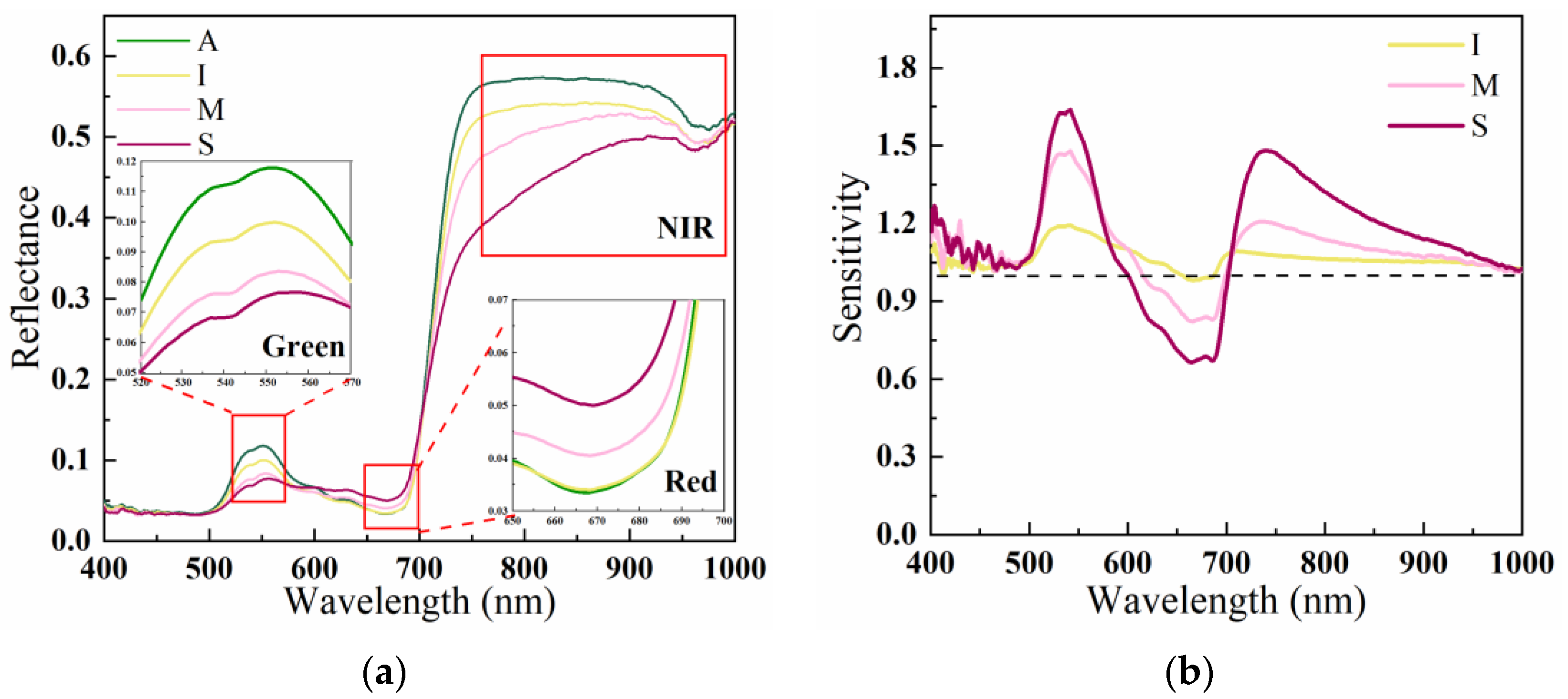
In this study, we evaluated the variability in wavelengths by analyzing the average spectral features and sensitivity of different disease levels. Our findings indicate that the wavelengths with the highest variability are primarily located in the green, red, and near-infrared bands. These results are consistent with those reported in [35]. Specifically, The authors of [36] proposed that the decline in reflectance in the green band could be attributed to the breakdown of chlorophyll. In addition, the variation in reflectance in the red band might be related to changes in carotenoid and lutein pigments. On the other hand, the authors of [37,38] suggested that the decline in reflectance in the NIR region is mainly influenced by changes in leaf structure and water content.
The studies of [39,
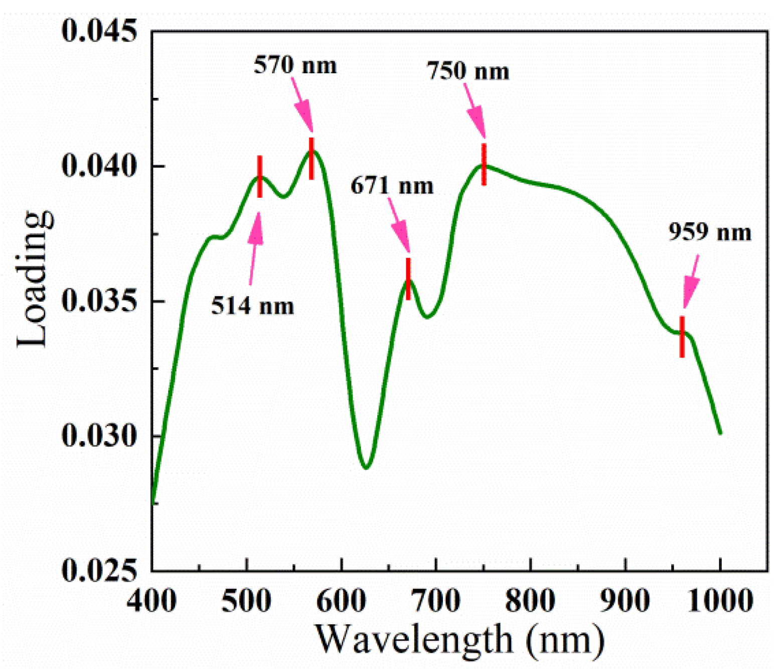
40] have shown that different crops and diseases have distinct spectral responses, and identifying specific feature wavelengths is crucial for accurate disease detection. Therefore, in this study, we used the proposed I-PCA loading method to assign weights to each wavelength, and we obtained high weight values in the ranges of 500–570 nm, 650–700 nm, and 760–1000 nm. We then used the local peak and correlation optimization method to select 570 nm, 671 nm, and 750 nm as feature wavelengths. Notably, 570 nm was in the green band, 671 nm was in the red band, and 750 nm was in the near-infrared band. These findings align with our analysis of spectral variability among disease levels.
Other studies have also used the feature wavelengths identified in this study. For example, the authors of [41] used 570 nm to detect FHB in late flowering, and the authors of [42] identified it as a crucial feature wavelength for detecting apple blasts. Additionally, 670 nm is commonly used to estimate leaf chlorophyll content and is a feature wavelength widely used in vegetation indices such as the NDVI [43], MSR [44], MCARI [45], TCARI [46], and OSAVI [47]. Additionally, 750 nm was identified by [48] as the most distinguishable part of the lesion detection spectrum. Our findings suggest that diseases cause changes in crops’ physiological and biochemical parameters, leading to distinct spectral responses. Identifying and utilizing specific feature wavelengths can greatly enhance disease detection accuracy.
This study employed eight feature selection methods to identify feature wavelengths, including CARS, LSMI, RF, Relief-F, the SPA, UVE, PCA loading, and I-PCA loading. We found that different methods produced different feature wavelengths, which can be attributed to the different evaluation criteria of the methods. Similar findings were reported by the Zhang [49] and Balabin [50], who used 10 and 16 optimal wavelength selection methods, respectively. Notably, the feature wavelengths identified by all methods were mostly concentrated in the green, red, red-edge, and near-infrared bands, consistent with variability in wavelengths. When we evaluated the feature wavelengths using KNNs, SVMs, and BP, we found that all models achieved satisfactory accuracy, with OA and Kappa exceeding 85% and 80%, respectively. Although different methods selected different feature wavelengths, these features were still concentrated in similar regions, demonstrating their ability to enhance detection capability. There were often cases of excessive and repetitive selection in methods with a larger number of selected feature wavelengths. For example, CARS and UVE selected 10 and 9 feature wavelengths, respectively. However, some of their selected feature wavelengths were concentrated between 400 and 420 nm and 980 and 1000 nm, which did not correspond with the results of wavelength difference analysis. Therefore, selecting too many feature wavelengths may not improve disease detection accuracy. In addition, the LSMI, SPA, and I-PCA loading methods were used for feature selection, and the results show that only three feature wavelengths were selected. The KNN, SVM, and BP algorithms were used to evaluate the disease detection ability of different feature wavelengths. The results showed that LSMI achieved an OA and Kappa of over 90% and 87%, respectively, with all classifiers. In comparison, the SPA achieved an OA and Kappa of over 87% and 83%, respectively, with all classifiers. Other studies have also demonstrated the effectiveness of the LSMI and SPA methods in feature selection [30,
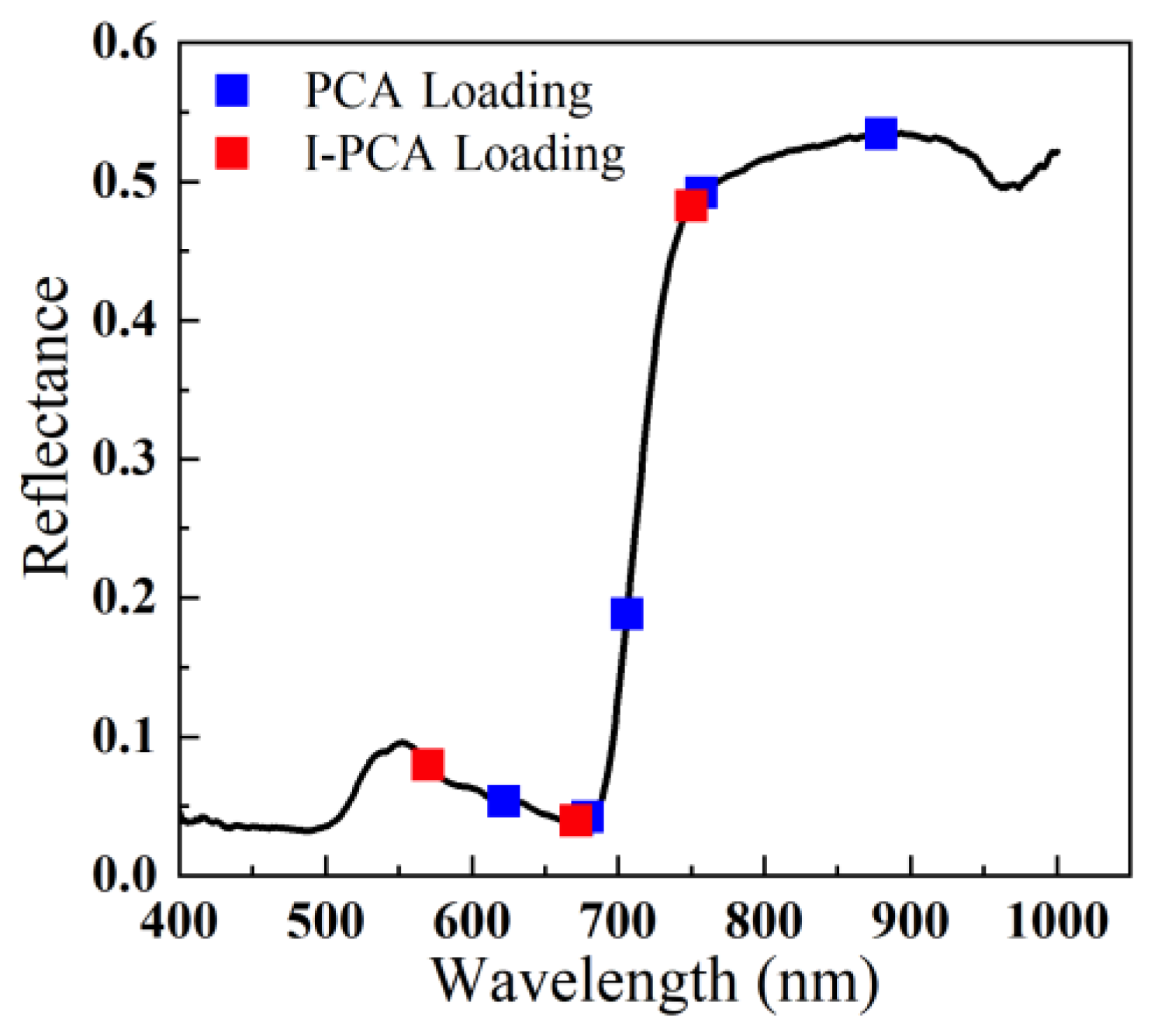
33]. Therefore, selecting fewer feature wavelengths can achieve higher disease detection accuracy. Similar to the LSMI and SPA methods, the three feature wavelengths selected in this study were located in the green, red, and near-infrared bands and detected with high a degree of accuracy. Furthermore, it can be seen from analysis of wavelength difference that the feature wavelengths selected in this study are better than those selected by the LSMI and SPA methods, which may be the reason why the selected feature wavelengths performed better in disease detection in this study.
In this study, various feature selection methods were evaluated using different classifiers, with I-PCA loading identified as the best-performing method. Specifically, the SVM classification results using feature wavelengths selected by I-PCA loading achieved high OA and Kappa scores of 96.88% and 95.81%, respectively. Further analysis of disease severity detection using the selected feature wavelengths, and the results are shown in Table 6. The results revealed that the HM values for all categories exceeded 96%, with the highest HM of 98.55% achieved for level S. More samples incorrectly predicted A levels as I levels, and fewer samples incorrectly predicted I levels as A levels, resulting in a PA below 95% and a UA above 98% for A levels. These results suggest that the model can accurately predict healthy areas, which can aid in the timely detection and control of crop diseases in real-world production settings.

6. Conclusions

This study collected spectral reflectance data for peanut leaf spot disease with different severity levels in the laboratory. It was found that disease severity significantly affects variability in wavelengths within the green, red, and near-infrared bands. This study proposed an improved PCA loading method and obtained three feature wavelengths at 570 nm, 671 nm, and 750 nm to identify the most important feature wavelengths. The proposed method was also compared with seven commonly used feature selection methods using KNN, SVM, and BP classifiers. Results showed that the proposed I-PCA loading method achieved higher classification accuracy with fewer feature wavelengths. The SVM classifier achieved the highest accuracy, with OA at 96.88% and Kappa at 95.81%. This study demonstrates that the proposed method effectively detects peanut leaf spot disease.

Author Contributions

Conceptualization, K.S. and T.X.; data curation, S.F.; formal analysis, K.S.; funding acquisition, T.X.; investigation, Q.G.; methodology, Q.G.; project administration, D.Z.; resources, T.X.; software, D.Z.; supervision, K.S.; validation, Q.G. and H.W.; visualization, H.W.; writing—original draft, Q.G.; writing—review and editing, K.S. All authors have read and agreed to the published version of the manuscript.

Funding

This research was partially funded by basic research funds for universities directly under the Inner Mongolia Autonomous Region (GXKY22133), Doctoral Startup Foundation of Inner Mongolia (BS658), Science and Technology Plan Project of Inner Mongolia Autonomous Region (2020GG0189), Central Government Guided Local Science and Technology Development Fund Project (2020ZY0003), Doctoral Startup Foundation of Inner Mongolia (BS603), and Higher Education Science Research Project of Inner Mongolia Autonomous Region of China (NJZY21419).

Conflicts of Interest

The authors declare that they have no conflict of interest.

References

  1. Khera, P.; Pandey, M.K.; Wang, H.; Feng, S.; Qiao, L.; Culbreath, A.K.; Kale, S.; Wang, J.; Holbrook, C.C.; Zhuang, W.; et al. Mapping quantitative trait loci of resistance to tomato spotted wilt virus and leaf spots in a recombinant inbred line population of peanut (Arachis hypogaea L.) from SunOleic 97R and NC94022. PLoS ONE 2016, 11, e0158452. [Google Scholar] [CrossRef]
  2. Chiteka, Z.A.; Gorbet, D.W.; Shokes, F.M.; Kucharek, T.A.; Knauft, D.A. Components of Resistance to Late Leafspot in Peanut. I. Levels and Variability-Implications for Selection1. Peanut Sci. 1988, 15, 25–30. [Google Scholar] [CrossRef]
  3. Mueller, D.S.; Bradley, C.A.; Grau, C.R.; Gaska, J.M.; Kurle, J.E.; Pedersen, W.L. Application of thiophanate-methyl at different host growth stages for management of sclerotinia stem rot in soybean. Crop Prot. 2004, 23, 983–988. [Google Scholar] [CrossRef]
  4. Partel, V.; Charan Kakarla, S.; Ampatzidis, Y. Development and evaluation of a low-cost and smart technology for precision weed management utilizing artificial intelligence. Comput. Electron. Agric. 2019, 157, 339–350. [Google Scholar] [CrossRef]
  5. Rahman, M.T.; Uddin, M.S.; Sultana, R.; Moue, A.; Setu, M. Polymerase chain reaction (PCR): A short review. Anwer Khan Mod. Med. Coll. J. 2013, 4, 30–36. [Google Scholar] [CrossRef]
  6. Butler, J.E. Enzyme-linked immunosorbent assay. J. Immunoass. 2000, 21, 165–209. [Google Scholar] [CrossRef] [PubMed]
  7. López, M.M.; Llop, P.; Olmos, A.; Marco-Noales, E.; Cambra, M.; Bertolini, E. Are molecular tools solving the challenges posed by detection of plant pathogenic bacteria and viruses? Curr. Issues Mol. Biol. 2009, 11, 13–46. [Google Scholar] [CrossRef] [PubMed]
  8. Martinelli, F.; Scalenghe, R.; Davino, S.; Panno, S.; Scuderi, G.; Ruisi, P.; Villa, P.; Stroppiana, D.; Boschetti, M.; Goulart, L.R.; et al. Advanced methods of plant disease detection. A review. Agron. Sustain. Dev. 2015, 35, 1–25. [Google Scholar] [CrossRef]
  9. Weiss, M.; Jacob, F.; Duveiller, G. Remote sensing for agricultural applications: A meta-review. Remote Sens. Environ. 2020, 236, 111402. [Google Scholar] [CrossRef]
  10. Pantazi, X.-E.; Moshou, D.; Bravo, C. Active learning system for weed species recognition based on hyperspectral sensing. Biosyst. Eng. 2016, 146, 193–202. [Google Scholar] [CrossRef]
  11. Khanal, S.; Fulton, J.; Shearer, S. An overview of current and potential applications of thermal remote sensing in precision agriculture. Comput. Electron. Agric. 2017, 139, 22–32. [Google Scholar] [CrossRef]
  12. Feng, S.; Zhao, D.; Guan, Q.; Li, J.; Liu, Z.; Jin, Z.; Li, G.; Xu, T. A deep convolutional neural network-based wavelength selection method for spectral characteristics of rice blast disease. Comput. Electron. Agric. 2022, 199, 107199. [Google Scholar] [CrossRef]
  13. Guan, Q.; Song, K.; Feng, S.; Yu, F.; Xu, T. Detection of peanut leaf spot disease based on leaf-, plant-, and field-scale hyperspectral reflectance. Remote Sens. 2022, 14, 4988. [Google Scholar] [CrossRef]
  14. Gu, Q.; Sheng, L.; Zhang, T.; Lu, Y.; Zhang, Z.; Zheng, K.; Hu, H.; Zhou, H. Early detection of tomato spotted wilt virus infection in tobacco using the hyperspectral imaging technique and machine learning algorithms. Comput. Electron. Agric. 2019, 167, 105066. [Google Scholar] [CrossRef]
  15. Meng, R.; Lv, Z.; Yan, J.; Chen, G.; Zhao, F.; Zeng, L.; Xu, B. Development of spectral disease indices for southern corn rust detection and severity classification. Remote Sens. 2020, 12, 3233. [Google Scholar] [CrossRef]
  16. Jiang, Q.; Wu, G.; Tian, C.; Li, N.; Yang, H.; Bai, Y.; Zhang, B. Hyperspectral imaging for early identification of strawberry leaves diseases with machine learning and spectral fingerprint features. Infrared Phys. Technol. 2021, 118, 103898. [Google Scholar] [CrossRef]
  17. Bauriegel, E.; Giebel, A.; Geyer, M.; Schmidt, U.; Herppich, W.B. Early detection of Fusarium infection in wheat using hyper-spectral imaging. Comput. Electron. Agric. 2011, 75, 304–312. [Google Scholar] [CrossRef]
  18. Kong, W.; Zhang, C.; Huang, W.; Liu, F.; He, Y. Application of Hyperspectral Imaging to Detect Sclerotinia sclerotiorum on Oilseed Rape Stems. Sensors 2018, 18, 123. [Google Scholar] [CrossRef]
  19. Li, J.; Luo, W.; Wang, Z.; Fan, S. Early detection of decay on apples using hyperspectral reflectance imaging combining both principal component analysis and improved watershed segmentation method. Postharvest Biol. Technol. 2019, 149, 235–246. [Google Scholar] [CrossRef]
  20. Wang, Z.; Tian, X.; Fan, S.; Zhang, C.; Li, J. Maturity determination of single maize seed by using near-infrared hyperspectral imaging coupled with comparative analysis of multiple classification models. Infrared Phys. Technol. 2021, 112, 103596. [Google Scholar] [CrossRef]
  21. Kong, W.; Zhang, C.; Cao, F.; Liu, F.; Luo, S.; Tang, Y.; He, Y. Detection of sclerotinia stem rot on oilseed rape (Brassica napus L.) leaves using hyperspectral imaging. Sensors 2018, 18, 1764. [Google Scholar] [CrossRef] [PubMed]
  22. Chen, T.; Yang, W.; Zhang, H.; Zhu, B.; Zeng, R.; Wang, X.; Wang, S.; Wang, L.; Qi, H.; Lan, Y.; et al. Early detection of bacterial wilt in peanut plants through leaf-level hyperspectral and unmanned aerial vehicle data. Comput. Electron. Agric. 2020, 177, 105708. [Google Scholar] [CrossRef]
  23. Dai, Q.; Cheng, J.-H.; Sun, D.-W.; Zeng, X.-A. Advances in Feature Selection Methods for Hyperspectral Image Processing in Food Industry Applications: A Review. Crit. Rev. Food Sci. Nutr. 2015, 55, 1368–1382. [Google Scholar] [CrossRef]
  24. Abdullah, M.Z.; Guan, L.C.; Mohd Azemi, B.M.N. Stepwise discriminant analysis for colour grading of oil palm using machine vision system. Food Bioprod. Process. 2001, 79, 223–231. [Google Scholar] [CrossRef]
  25. Burges, C.J.C. A Tutorial on Support Vector Machines for Pattern Recognition. Data Min. Knowl. Discov. 1998, 2, 121–167. [Google Scholar] [CrossRef]
  26. Wang, Y.; Niu, D.; Ji, L. Short-term power load forecasting based on IVL-BP neural network technology. Syst. Eng. Procedia 2012, 4, 168–174. [Google Scholar] [CrossRef]
  27. Yuan, L.; Yan, P.; Han, W.; Huang, Y.; Wang, B.; Zhang, J.; Zhang, H.; Bao, Z. Detection of anthracnose in tea plants based on hyperspectral imaging. Comput. Electron. Agric. 2019, 167, 105039. [Google Scholar] [CrossRef]
  28. Zhang, J.-C.; Pu, R.-l.; Wang, J.-h.; Huang, W.-j.; Yuan, L.; Luo, J.-h. Detecting powdery mildew of winter wheat using leaf level hyperspectral measurements. Comput. Electron. Agric. 2012, 85, 13–23. [Google Scholar] [CrossRef]
  29. Li, H.; Liang, Y.; Xu, Q.; Cao, D. Key wavelengths screening using competitive adaptive reweighted sampling method for multivariate calibration. Anal. Chim. Acta 2009, 648, 77–84. [Google Scholar] [CrossRef]
  30. Suzuki, T.; Sugiyama, M.; Kanamori, T.; Sese, J. Mutual information estimation reveals global associations between stimuli and biological processes. BMC Bioinform. 2009, 10, S52. [Google Scholar] [CrossRef] [PubMed]
  31. Li, H.-D.; Xu, Q.-S.; Liang, Y.-Z. Random frog: An efficient reversible jump Markov Chain Monte Carlo-like approach for variable selection with applications to gene selection and disease classification. Anal. Chim. Acta 2012, 740, 20–26. [Google Scholar] [CrossRef]
  32. Robnik-Šikonja, M.; Kononenko, I. Theoretical and empirical analysis of ReliefF and RReliefF. Mach. Learn. 2003, 53, 23–69. [Google Scholar] [CrossRef]
  33. Araújo, M.C.U.; Saldanha, T.C.B.; Galvao, R.K.H.; Yoneyama, T.; Chame, H.C.; Visani, V. The successive projections algorithm for variable selection in spectroscopic multicomponent analysis. Chemom. Intell. Lab. Syst. 2001, 57, 65–73. [Google Scholar] [CrossRef]
  34. Centner, V.; Massart, D.-L.; de Noord, O.E.; de Jong, S.; Vandeginste, B.M.; Sterna, C. Elimination of uninformative variables for multivariate calibration. Anal. Chem. 1996, 68, 3851–3858. [Google Scholar] [CrossRef] [PubMed]
  35. Chen, T.; Zhang, J.; Chen, Y.; Wan, S.; Zhang, L. Detection of peanut leaf spots disease using canopy hyperspectral reflectance. Comput. Electron. Agric. 2019, 156, 677–683. [Google Scholar] [CrossRef]
  36. Devadas, R.; Lamb, D.W.; Simpfendorfer, S.; Backhouse, D. Evaluating ten spectral vegetation indices for identifying rust infection in individual wheat leaves. Precis. Agric. 2009, 10, 459–470. [Google Scholar] [CrossRef]
  37. Gitelson, A.A.; Kaufman, Y.J.; Stark, R.; Rundquist, D. Novel algorithms for remote estimation of vegetation fraction. Remote Sens. Environ. 2002, 80, 76–87. [Google Scholar] [CrossRef]
  38. Jacquemoud, S.; Baret, F. PROSPECT: A model of leaf optical properties spectra. Remote Sens. Environ. 1990, 34, 75–91. [Google Scholar] [CrossRef]
  39. Ashourloo, D.; Mobasheri, M.R.; Huete, A. Developing two spectral disease indices for detection of wheat leaf rust (Pucciniatriticina). Remote Sens. 2014, 6, 4723–4740. [Google Scholar] [CrossRef]
  40. Mahlein, A.K.; Rumpf, T.; Welke, P.; Dehne, H.W.; Plümer, L.; Steiner, U.; Oerke, E.C. Development of spectral indices for detecting and identifying plant diseases. Remote Sens. Environ. 2013, 128, 21–30. [Google Scholar] [CrossRef]
  41. Zhang, D.; Wang, Q.; Lin, F.; Yin, X.; Gu, C.; Qiao, H. Development and Evaluation of a New Spectral Disease Index to Detect Wheat Fusarium Head Blight Using Hyperspectral Imaging. Sensors 2020, 20, 2260. [Google Scholar] [CrossRef] [PubMed]
  42. Delalieux, S.; Somers, B.; Verstraeten, W.W.; van Aardt, J.A.N.; Keulemans, W.; Coppin, P. Hyperspectral indices to diagnose leaf biotic stress of apple plants, considering leaf phenology. Int. J. Remote Sens. 2009, 30, 1887–1912. [Google Scholar] [CrossRef]
  43. Rouse, J.W., Jr.; Haas, R.H.; Schell, J.A.; Deering, D.W. Monitoring Vegetation Systems in the Great Plains with Erts. NASA Spec. Publ. 1974, 351, 309. [Google Scholar]
  44. Chen, J.M. Evaluation of Vegetation Indices and a Modified Simple Ratio for Boreal Applications. Can. J. Remote Sens. 1996, 22, 229–242. [Google Scholar] [CrossRef]
  45. Haboudane, D.; Miller, J.R.; Pattey, E.; Zarco-Tejada, P.J.; Strachan, I.B. Hyperspectral vegetation indices and novel algorithms for predicting green LAI of crop canopies: Modeling and validation in the context of precision agriculture. Remote Sens. Environ. 2004, 90, 337–352. [Google Scholar] [CrossRef]
  46. Haboudane, D.; Miller, J.R.; Tremblay, N.; Zarco-Tejada, P.J.; Dextraze, L. Integrated narrow-band vegetation indices for prediction of crop chlorophyll content for application to precision agriculture. Remote Sens. Environ. 2002, 81, 416–426. [Google Scholar] [CrossRef]
  47. Rondeaux, G.; Steven, M.; Baret, F. Optimization of soil-adjusted vegetation indices. Remote Sens. Environ. 1996, 55, 95–107. [Google Scholar] [CrossRef]
  48. Van De Vijver, R.; Mertens, K.; Heungens, K.; Somers, B.; Nuyttens, D.; Borra-Serrano, I.; Lootens, P.; Roldán-Ruiz, I.; Vangeyte, J.; Saeys, W. In-field detection of Alternaria solani in potato crops using hyperspectral imaging. Comput. Electron. Agric. 2020, 168, 105106. [Google Scholar] [CrossRef]
  49. Zhang, C.; Jiang, H.; Liu, F.; He, Y. Application of Near-Infrared Hyperspectral Imaging with Variable Selection Methods to Determine and Visualize Caffeine Content of Coffee Beans. Food Bioprocess Technol. 2017, 10, 213–221. [Google Scholar] [CrossRef]
  50. Balabin, R.M.; Smirnov, S.V. Variable selection in near-infrared spectroscopy: Benchmarking of feature selection methods on biodiesel data. Anal. Chim. Acta 2011, 692, 63–72. [Google Scholar] [CrossRef]
Figure 1. Location and overview of the experimental site.
Agronomy 13 01153 g001
Figure 2. Collection equipment and leaf samples.
Agronomy 13 01153 g002
Figure 3. Average reflectance and sensitivity for different leaf spot disease levels. (a) Average reflectance, (b) sensitivity.
Agronomy 13 01153 g003
Figure 4. Scatter plot and statistical histogram of combinations between the first five principal components. PC: principal component.
Agronomy 13 01153 g004
Figure 5. Loading coefficient curves of each principal component and the selected feature wavelengths. (a) PC1, (b) PC2, (c) PC3.
Agronomy 13 01153 g005
Figure 6. Loading coefficient curves of the improved PCA loading method and the selected feature wavelengths.
Agronomy 13 01153 g006
Figure 7. Feature wavelengths selected by conventional PCA loading and improved PCA loading.
Agronomy 13 01153 g007
Figure 8. Classification results of the feature wavelengths selected by PCA loading and I-PCA loading. (a) and (b) are OA and Kappa for KNNs, (c) and (d) are OA and Kappa for SVMs, and (e) and (f) are OA and Kappa for BP.
Agronomy 13 01153 g008
Table 1. Disease severity levels at leaf scale.
LevelDisease SeverityArea Ratio
AAsymptomatic 0
IInitially symptomatic 0 0.1
MModerately symptomatic 0.1 0.25
SSeverely symptomatic 0.25 0.5
Table 2. Confusion matrix.
Predicted ClassActual Class
AIMSTotalsUA
A X 11 X 12 X 13 X 14 i = 1 4 X 1 i X 11 i = 1 4 X 1 i
I X 21 X 22 X 23 X 24 i = 1 4 X 2 i X 22 i = 1 4 X 2 i
M X 31 X 32 X 33 X 34 i = 1 4 X 3 i X 33 i = 1 4 X 3 i
S X 41 X 42 X 43 X 44 i = 1 4 X 4 i X 44 i = 1 4 X 4 i
Totals i = 1 4 X i 1 i = 1 4 X i 2 i = 1 4 X i 3 i = 1 4 X i 4
PA X 11 i = 1 4 X i 1 X 22 i = 1 4 X i 2 X 33 i = 1 4 X i 3 X 44 i = 1 4 X i 4
A: asymptomatic; I: initially symptomatic; M: moderately symptomatic; S: severely symptomatic.
Table 3. Eigenvalues, contribution rates, and cumulative contribution rates of each principal component.
PCsEigenvaluesContribution Rate (%)Cumulative Contribution Rate (%)
PC1339.3956.4756.47
PC2158.1726.3282.79
PC343.137.17889.97
PC426.604.4394.39
PC59.291.5595.94
PC: principal component.
Table 4. Results of different feature wavelength selection methods.
MethodsNumber of WavelengthsFeature Wavelengths (nm)
CARS10404, 411, 435, 504, 534, 584, 667, 884, 989, 996
LSMI3519, 667, 850
RF6465, 536, 626, 701, 932, 997
Relief-F7412, 421, 458, 540, 660, 760, 996
SPA3547, 696, 958
UVE9405, 412, 489, 534, 595, 682, 882, 988, 999
PCA Loading6626, 672, 679, 706, 757, 880
I-PCA Loading3570, 671, 750
Table 5. Classification results of feature wavelength selection methods.
MethodsKNNSVMBP
OA (%)Kappa (%)OA (%)Kappa (%)OA (%)Kappa (%)
CARS90.3486.9295.3393.7195.3793.78
LSMI90.6587.3593.7791.6092.7390.19
RF88.1683.9894.0892.0194.0391.96
Relief-F95.0293.2897.5196.6596.7395.60
SPA87.8583.5792.5289.9591.4888.55
UVE90.9787.7896.2694.9795.4293.83
PCA Loading94.7092.8596.5795.3996.9895.93
I-PCA Loading95.3393.7096.8895.8195.7394.26
OA: overall accuracy; Kappa: kappa coefficient.
Table 6. Confusion matrix for detecting disease severity based on an SVM.
Predicted ClassActual Class
AIMSTotalsUA (%)
A741007598.67%
I4992010594.29%
M017127495.95%
S0006767100.00%
Totals781017369321
PA (%)94.87%98.02%97.26%97.10% OA = 96.88%
HM (%)96.77%96.15%96.60%98.55% Kappa = 95.81%
A: asymptomatic; I: initially symptomatic; M: moderately symptomatic; S: severely symptomatic; UA: user’s accuracy; PA: producer’s accuracy; HM: harmonic mean; OA: overall accuracy; Kappa: kappa coefficient.
Disclaimer/Publisher’s Note: The statements, opinions and data contained in all publications are solely those of the individual author(s) and contributor(s) and not of MDPI and/or the editor(s). MDPI and/or the editor(s) disclaim responsibility for any injury to people or property resulting from any ideas, methods, instructions or products referred to in the content.

