Estimation of Leaf Area Index and Above-Ground Biomass of Winter Wheat Based on Optimal Spectral Index

Abstract

Leaf area index (LAI) and above-ground biomass are both vital indicators for evaluating crop growth and development, while rapid and non-destructive estimation of crop LAI and above-ground biomass is of considerable significance for crop field management. Owing to the advantages of repeatable and high-throughput observations, spectral technology provides a feasible method for obtaining LAI and above-ground biomass of crops. In the present study, the spectral, LAI and above-ground biomass data of winter wheat were collected, and 7 species (14 in total) were calculated based on the original and first-order differential spectrum correlation spectral indices with LAI. Then, the correlation matrix method was used for correlation with LAI. The optimal wavelength combination was extracted, and the results were calculated as the optimal spectral index related to LAI. The calculation process of the optimal spectral index related to above-ground biomass was the same as that aforementioned. Finally, the optimal spectral index was divided into three groups of model input variables, winter wheat LAI and above-ground biomass estimation models were constructed using support vector machine (SVM), random forest (RF) and a back propagation neural network (BPNN), and the models were verified. The results show that the correlation coefficient between the highest of the optimal spectral indices, the LAI, and the above-ground biomass of winter wheat exceeded 0.6, and the correlation was good. The methods for establishing the optimal estimation models for LAI and above-ground biomass of winter wheat are all modeling methods in which the input variables are the combination of the first-order differential spectral index (combination 2) and RF. The R² of the LAI estimation model validation set was 0.830, the RMSE was 0.276, and the MRE was 6.920; the R² of the above-ground biomass estimation model validation set was 0.682, RMSE was 235.016, MRE was 4.336, and the accuracies of both models were high. The present research results can provide a theoretical basis for crop monitoring based on spectral technology and provide an application reference for the rapid estimation of crop growth parameters.

1. Introduction

Leaf area index (LAI) is a significant vegetation parameter that characterizes leaf density and canopy structure. LAI is widely used in models for climate change, net primary productivity, and crop growth, being closely related to crop transpiration, light energy interception, photosynthetic rate, net primary productivity, and other parameters. In ecological model and water and carbon cycle research, LAI is generally regarded as a significant factor, LAI is generally regarded as a significant factor that is used to reflect the number of plant leaves, changes in canopy structure, plant community vitality, and environmental effects. In addition, it provides structured quantitative information for the description of plant canopy surface material and energy exchange [1,2]. Biomass is the product of photosynthesis in the process of crop growth and development, which can reflect crop growth and nutritional status, which is a significant basis for crop yield formation [3,4]. According to the above-ground LAI and biomass, crop growth monitoring and yield forecast can be conducted, in addition to field water and fertilizer management [5,6,7]. As such, quick and accurate determination of the above-ground LAI and biomass is of considerable significance.

The traditional acquisition of above-ground biomass and LAI of crops is mainly achieved through destructive manual measurement, and the process is cumbersome, time-consuming and laborious. Thus, the popularization and application of such acquisition have been difficult to realize in large areas. In recent years, remote sensing technology has been gradually applied to the extraction of crop physiological and ecological parameters, which can potentially facilitate rapid acquisition of parameters such as crop biomass and LAI [8,9,10]. For the inversion method of vegetation chlorophyll content, the multivariate regression inversion method was gradually converted to the empirical/semi-empirical spectral index inversion method. At the same time, several scholars used the physical model method for inversion, but due to the complexity of the physical model inversion algorithm and numerous uncertain factors, many input parameters were difficult to obtain, resulting in limited inversion accuracy [11]. In contrast, the method of establishing an inversion model based on the spectral indices constructed by linear or nonlinear combinations of two or more spectral bands not only reflects the spectral information with better sensitivity than that of a single band, but can also be used in a certain range. Through such a method, the problem of band overfitting caused by using too many bands is eliminated to a certain extent, and the statistical analysis results are more accurate and convincing. Thus, such a method has been extensively adopted for the inversion of vegetation physiological and biochemical parameters [12].

The spectral index can quantitatively reflect and evaluate various indicators of crop growth, and establish a quantitative model between the spectral index and the physiological and biochemical indicators of crops [13]. In previous studies on the estimation of crop LAI and above-ground biomass using spectral indices, a number of scholars used fixed wavelengths to calculate spectral indices [9]. In addition, said scholars performed correlation analysis with LAI and above-ground biomass, and finally selected the spectral indices with better correlation. However, for different research objects, due to the different growth environments, growth periods and other factors, the physiological information of the crop itself will be different, resulting in different spectral characteristics. In such circumstances, using the same wavelength may cause the spectral data to be underutilized. The inversion model of the calculated spectral index has certain limitations, and the accuracy of the model will also be restricted to a certain extent. The jointing stage is a critical growth period of winter wheat, which marks the beginning of the differentiation of the floret primordium. As a vigorous growth period in which reproductive growth and vegetative growth are closely associated. Sufficient water, nutrients and light conditions are required to improve the tillering rate. To solve the above problems, in the present study, the LAI and above-ground biomass of wheat at the jointing stage were selected as the research objects, and the correlation matrix method was used to screen the characteristic wavelengths of spectral indices, so that the characteristic wavelengths had the highest correlation with the LAI and above-ground biomass of winter wheat used. Finally, 14 spectral indices and three regression methods were combined to construct a model, and the influence of the combination of different spectral indices and modeling methods on the accuracy of inversion of winter wheat LAI and above-ground biomass was discussed. The present results provide a theoretical basis for the study of accurate, non-destructive and rapid detection technology for LAI and above-ground biomass of winter wheat.

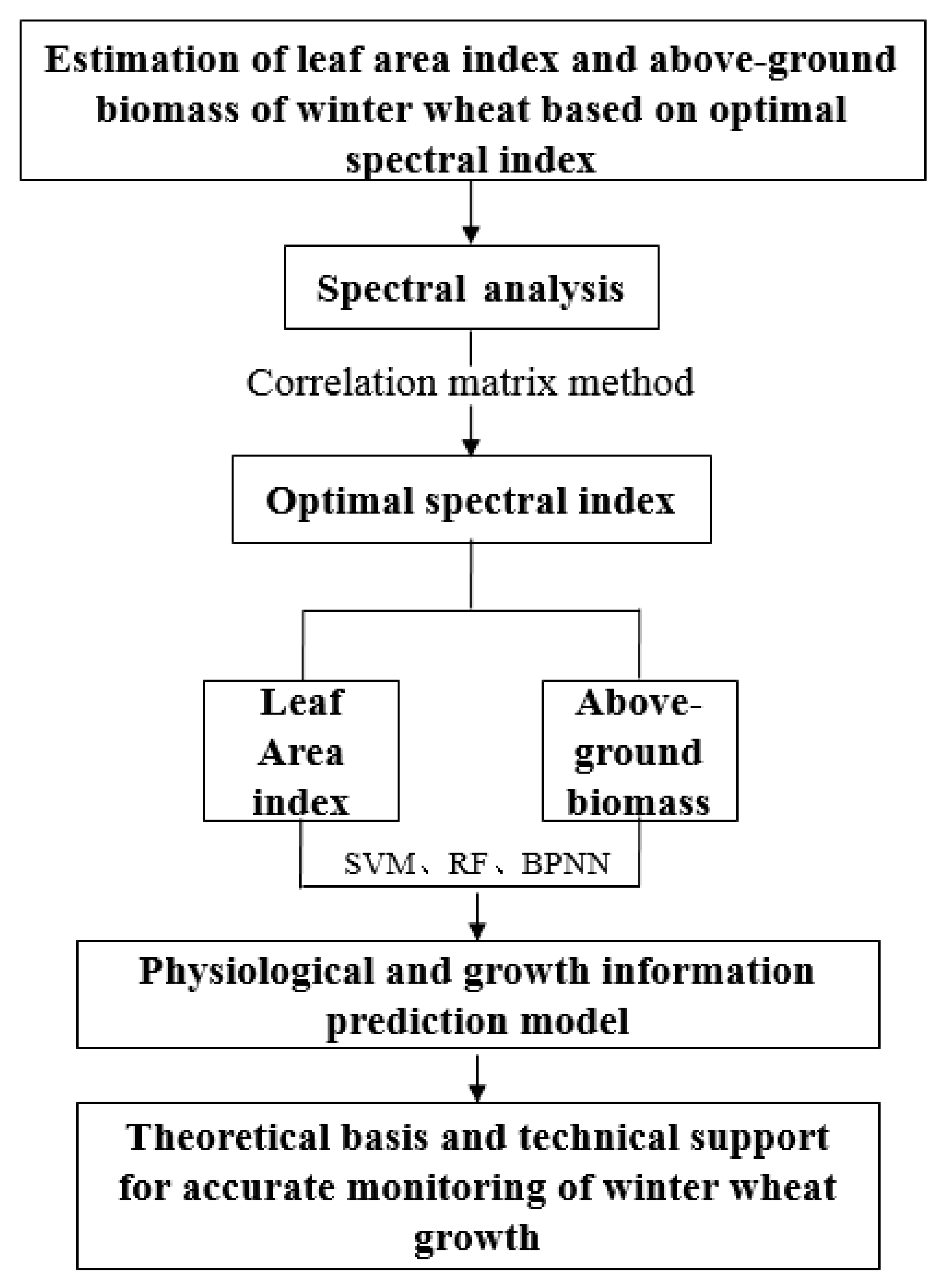
2. Materials and Methods

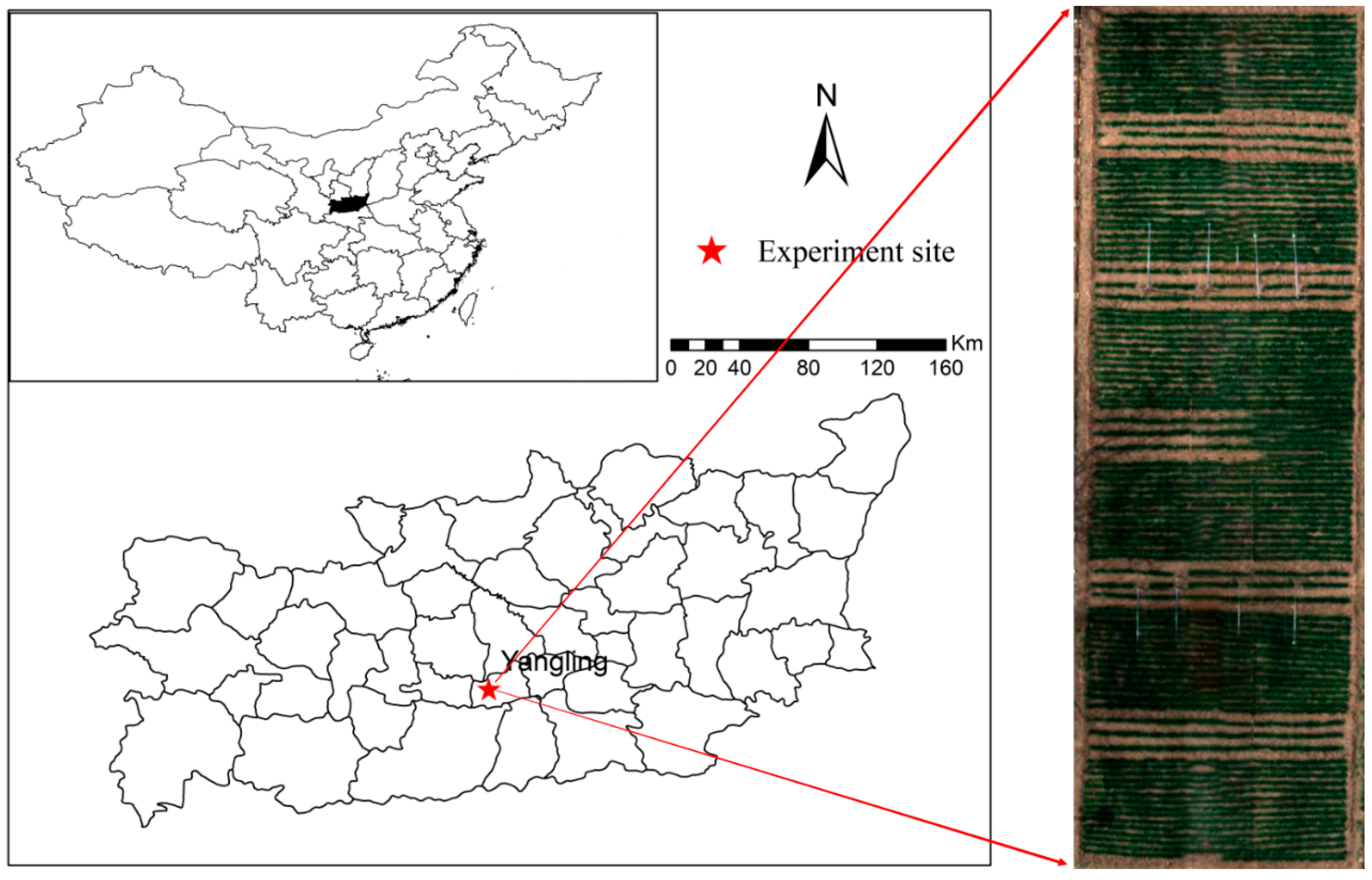
2.1. Research Area and Test Design

A two-year field experiment was conducted on winter wheat in 2018 and 2019 at the Water-saving Station of the Key Laboratory of Agricultural Soil and Water Engineering in Arid and Semiarid Areas of the Ministry of Education, Northwest A&F University, Yangling, China (34°18′ N, 108°24′ E, 521 m a.s.l.) (Figure 1). The area is a semi-humid but drought-prone region with annual average rainfall of 632 mm and potential evaporation of 1500 mm. There were a total of 34 test plots in the sampling area, and each test plot measured 7 m in length and 3 m in width. The planted winter-wheat variety was Xiaoyan 22. Four nitrogen fertilization levels of 100 kg N/hm² (N1), 160 kg N/hm² (N2), 220 kg N/hm² (N3) and 280 kg N/hm² (N4), and four fertilization types of Urea (U), slow-release fertilizer (SRF), UNS1 (U/SRF = 3/7) and UNS2 (U/SRF = 2/8) were setup. No nitrogen fertilizer was used as the control treatment (CK). The experiment was arranged in a completely randomized design with two replicates. The N fertilizer, phosphate fertilizer (120 kg P₂O₅ ha^–1) and potassium fertilizer (100 kg K₂O ha^–1) were applied as basal fertilizers and were incorporated into the 0–15 cm soil layer before planting. Winter wheat (Xiaoyan 22) was planted at 180 kg/hm².Wheat was seeded on October 15 in 2018 and October 15 in 2019, and harvested on June 25 in 2019 and 2020.

2.2. Data Collection

Ground-based LAI, above-ground biomass, and spectral data were obtained in the experimental plots during the winter wheat silking stage (31 March 2019 and 3 April 2020). Over the two-year experiment, 68 groups of LAI, above-ground biomass, and spectral reflectance samples were obtained. After removing outliers, 66 samples remained. Next, the LAI and above-ground biomass of winter wheat were sorted from small to large. Two-thirds of the samples were randomly selected as the modeling set, while the remaining one-third were used as the validation set. A summary of the number of samples in the modeling and validation sets, leaf area index, and statistical characteristics of above-ground biomass are displayed in

Table 1. Statistics of leaf area index and above-ground biomass in summer maize vegetation growth stage.

Indexes	Leaf Area Index/(cm2·cm−2)		Above-Ground Biomass/(kg·hm−2)
	Modeling Set	Validation Set	Modeling Set	Validation Set
Sample size	44	22	44	22
Minimum values	2.28	2.30	3247.20	3251.81
Maximum values	4.23	4.23	5073.49	4795.8
Mean	3.17	3.24	4159.26	4164.51
Standard deviation	0.59	1.62	442.53	405.87
Coefficient of variation/%	0.19	0.50	0.11	0.10

.

2.2.1. Measurement of LAI

In the present study, LAI was determined by means of a LAI-2000 Plant Canopy Analyzer [14], which is widely used for LAI measurements in the field. For the same developmental stages when canopy reflectance was collected, LAI measurements were conducted in all 34 wheat plots. Each plot was measured six times and the average was used as the plot LAI.

2.2.2. Above-Ground Biomass

Three plant samples were randomly taken from each plot at the silking stage. Wheat samples were put in an oven at 105 °C for 0.5 h and subsequently dried at 75 °C to constant weight. Wheat mass was then measured by an electronic balance.

2.2.3. Acquisition of Spectral Data

With each sampling for LAI and above-ground biomass, canopy spectra of sample points were acquired using a spectroradiometer (ASD Field-Spec^® 3 Standard-Res, Inc., Longmont, CO, USA). The spectral range was 350–1830 nm, covering the wavebands of 350–1000 nm with 3 nm resolution and the other wavebands with 10 nm resolution. The sensor had a 25° field of view, and the handheld probe was pointed vertically downward, with the instrument held 80 cm above the crop canopy. A representative plant canopy was selected for each test plot, and spectral values were collected 10 times. After removing nonstandard values, an average value was used as the final spectrum of the test plot. Spectral measurements were conducted on sunny and windless days between 11:00 a.m. and 2:00 p.m. to ensure comparability. A white spectral on reference reflectance panel (Labsphere, Inc., Longmont, CO, USA) reading was taken every 5 min or whenever required considering the changes in illumination conditions and used to convert digital number readings to reflectance. To reduce or eliminate the influence of useless information such as background noise, baseline drift, and stray light on the spectral reflectance curve, we used Savitzky–Golay convolution smoothing (9 points and 4 times) to preprocess the spectral data [15].

2.3. Techniques for Data Analysis

In the present study, 7 typical spectral indices were selected and the wavelength combination with the highest performance was chosen separately, so as to extract the correlation more accurately from the LAI and the above-ground biomass related to the spectral index. In the full spectrum wavelength range of 350–1830 nm, the spectral indices of all wavelength combinations in the original spectral data and the data obtained by first-order differentiation of the original spectral data were calculated, respectively (14 in total). The formula for calculating the spectral index is shown in

Table 2. Spectral index in this study. All indices were calculated from reflectance collected by spectroradiometer. i and j represent arbitrary wavelength positions, $R$ and $R$ represent the original wavelength positions of i and j. The initial spectral reflectance, $R$’ and $R$’ represent the first-order differential spectrum at the i and j wavelength positions Spectral reflectance, $R$₄₄₅ and $R$₅₅₀ represent the original spectrum at 445 and 550 nm wavelength positions spectral reflectance, $R$’₄₄₅ and $R$’₅₅₀ represent the first order at the 445 and 550 nm wavelength positions differential spectral reflectance.

Spectral Index	Formula		Reference
	Original	First-Order Differential
difference index (DI)	$R_i-R_j$	$R_i^{\prime }-R_j^{\prime }$	[12]
ratio index (RI)	$\frac{R_i}{R_j}$	$\frac{R_i^{\prime }}{R_j^{\prime }}$	[12]
normalized difference vegetation index (NDVI)	$\frac{R_i-R_j}{R_i+R_j}$	$\frac{R_i^{\prime }-R_j^{\prime }}{R_i^{\prime }+R_j^{\prime }}$	[12]
soil-adjusted vegetation index (SAVI)	$\left(1+0.16\right)\frac{R_i-R_j}{R_i+R_j+0.16}$	$\left(1+0.16\right)\frac{R_i^{\prime }-R_j^{\prime }}{R_i^{\prime }+R_j^{\prime }+0.16}$	[12]
triangular vegetation index (TVI)	$0.5\times \left(120\times \left(R_i-R_{550}\right)-200\times \left(R_j-R_{550}\right)\right)$	$0.5\times \left(120\times \left(R_i^{\prime }-R_{550}^{\prime }\right)-200\times \left(R_j^{\prime }-R_{550}^{\prime }\right)\right)$	[12]
modified simple ratio (mSR)	$\frac{R_i-R_{445}}{R_j-R_{445}}$	$\frac{R_i^{\prime }-R_{445}^{\prime }}{R_j^{\prime }-R_{445}^{\prime }}$	[12]
modified normalized difference index (mNDI)	$\frac{R_i-R_j}{R_i+R_j-2R_{445}}$	$\frac{R_i^{\prime }-R_j^{\prime }}{R_i^{\prime }+R_j^{\prime }-2R_{445}}$	[12]

, R_i and R_j represent the original wavelength positions of i and j; R_i’ and R_j’ represent the first-order differential spectrum at the i and j wavelength positions. All spectral index calculation results were obtained using MATLAB R2022a software(MathWorks, Inc. Natick, MA, USA) and all figures in the present article were obtained using Origin Pro 2021 software (OriginLab Corp., Northampton, MA, USA).

Three machine-learning methods, namely the support vector machine (SVM) [16], random forest (RF) model [17], and back propagation neutral network (BPNN) [18] were also tested using MATLAB R2022a software. In this study, the kernel function type of the SVM model was set to “poly”, and the parameter penalty coefficients C and γ of the SVM model were optimized using the grid search method. According to the principle of minimum cross-validation error, C and γ were determined to be 20 and 0.02, respectively [19]. In the construction of the RF model, the number of decision trees in the LAI model and the above-ground biomass model were both set to 500 after parameter optimization and multiple training [15]. The BPNN used in this study was provided by the Neural Network Toolbox in MATLAB. The transfer function of the hidden layer was set to TANSIG, and the Levenbeger–Marquardt (Train-LM) algorithm based on numerical optimization theory was used as the network training function. The number of neurons in the middle layer directly affects the simulation performance of the network. Thus, after several trainings, we determined that the number of neurons in the middle layer was 15. Also, during training, the maximum number of iterations was set to 1000 and the training target was set to 1 × 10⁻⁵. After the neural network was trained, the test data were entered into the training network simulation to obtain the simulated values. Average values of the data fitting results over the three periods were regarded as the model fitting results [20]. The 14 optimal spectral indices were divided into 3 groups as model input variables, the first group of variables was composed of 5 optimal spectral indices calculated from the original reflection spectrum, the second group of variables was composed of the 5 optimal spectral indices calculated from the first-order differential reflection spectrum and the third group of variables consisted of the top 5 spectral indices for all R_max values in the table. A standard two-layer feed-forward network with sigmoid transfer functions was chosen for the BPNN method [21], and SVM with the kernel function of Gaussian function [22] was tested in the present study.

2.4. Verify the Prediction Accuracy of the Models

In order to verify the prediction accuracy and predictive ability of the models, three indicators were selected, determination coefficient (R²), root mean square error (RMSE) and mean relative error (MRE), to evaluate the model accuracy [23]. The R², RMSE and MRE were calculated as follows:

$$R^2=\frac{{{\displaystyle \sum }}_{\dot{i}=1}^n{\left({\widehat{y}}_i-\overline{y}\right)}^2}{{{\displaystyle \sum }}_{i=1}^n{\left(y_i-\overline{y}\right)}^2}$$

(1)

$$RMSE=\sqrt{\frac{{{\displaystyle \sum }}_{i=1}^n{\left({\widehat{y}}_i-y_i\right)}^2}{n}}$$

(2)

$$MRE=\frac{1}{n}{{\displaystyle \sum }}_{i=1}^n\frac{\left|{\widehat{y}}_i-y_i\right|}{y_i}\times 100\%$$

(3)

where n is the number of samples; ${\widehat{y}}_i$ is the predicted value; $y_i$ is the observed value, and $\overline{y}$ is the average value. Diagrams of architectures used in the experiments is shown in Figure 2.

3. Results

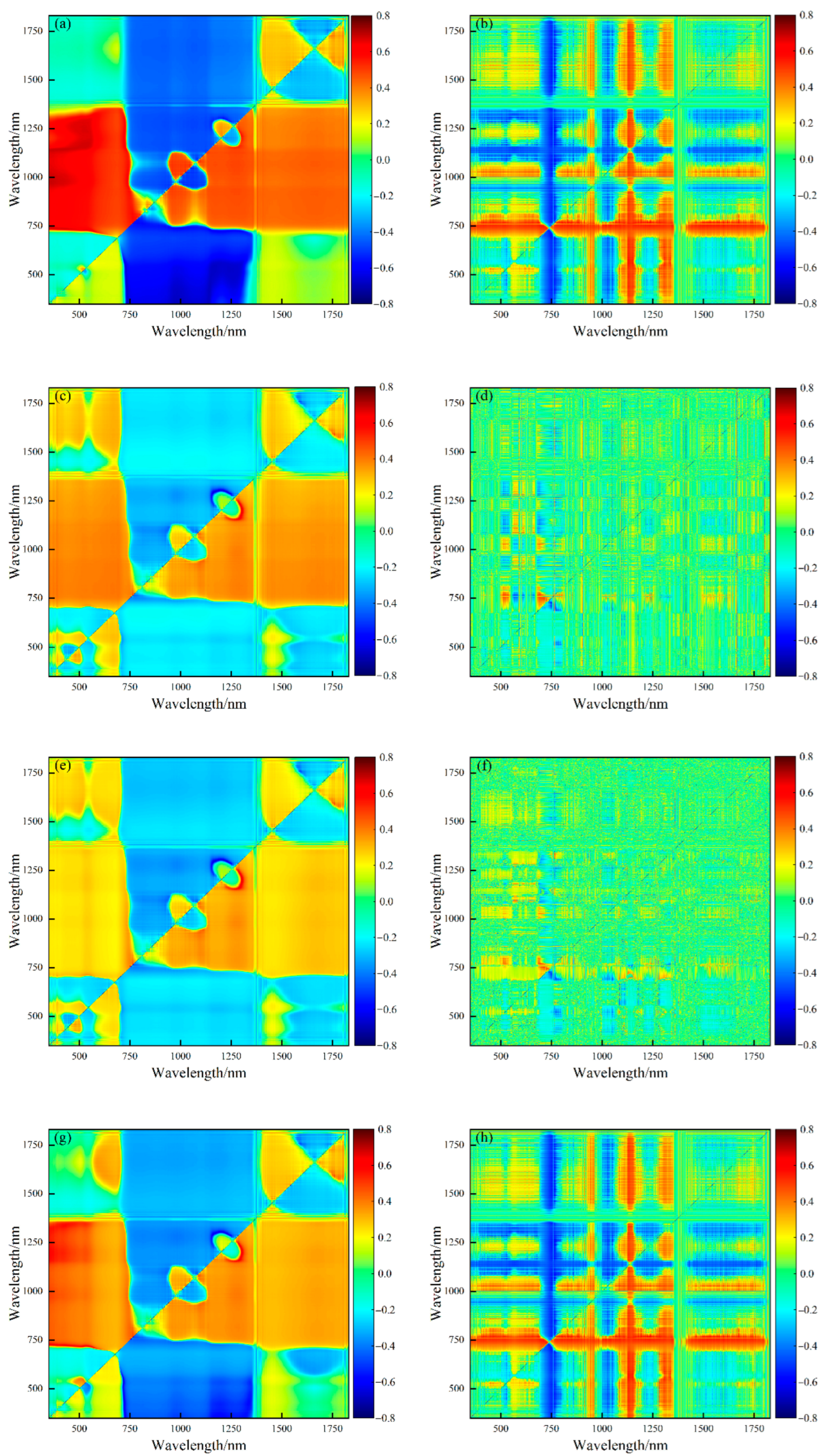
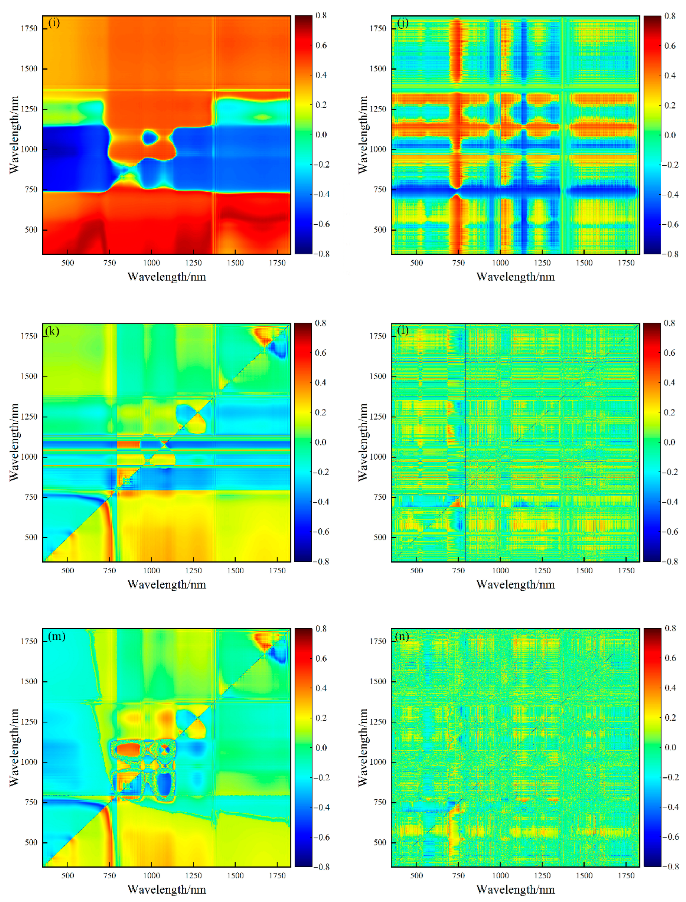
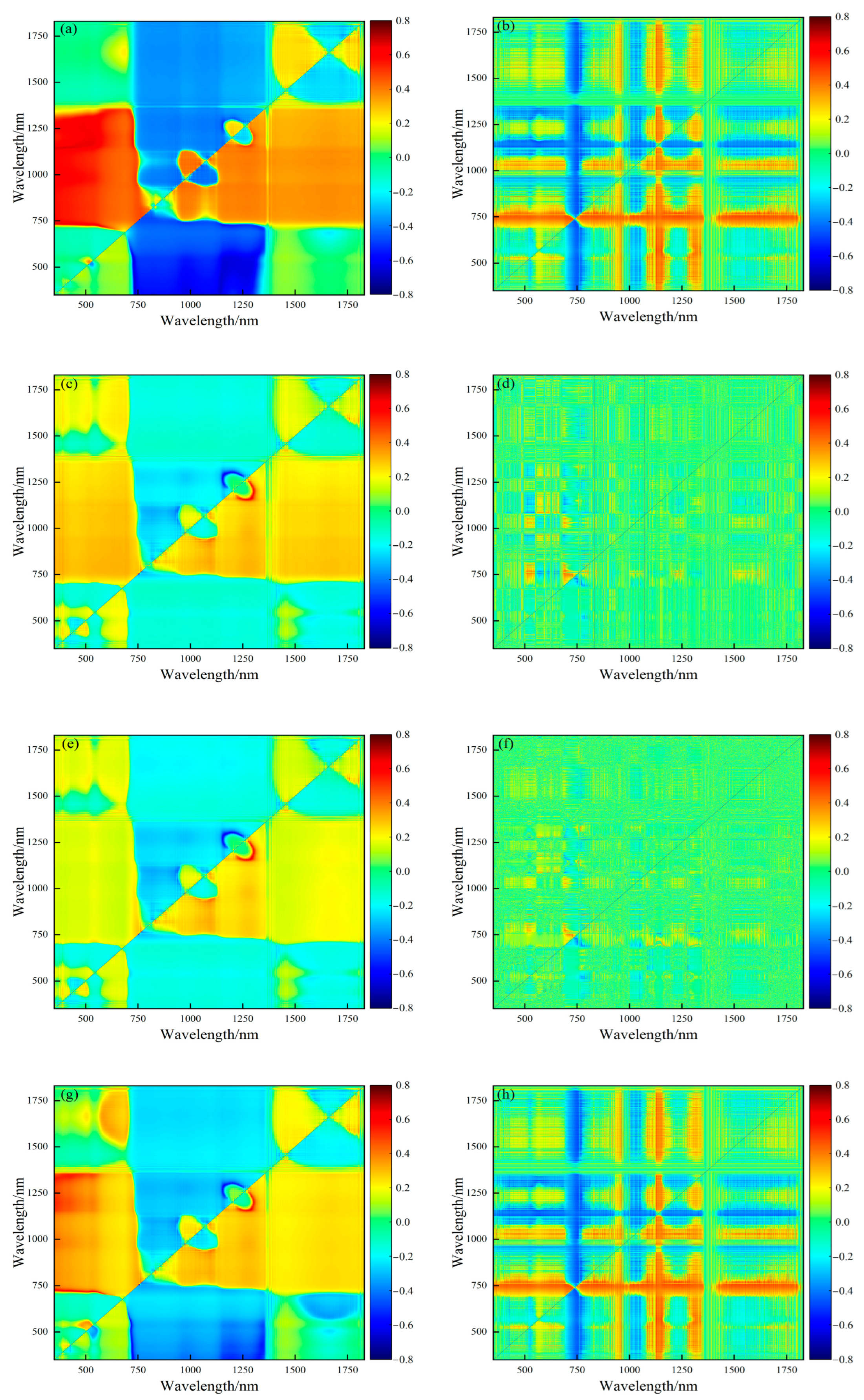
3.1. Extraction of Optimal Spectral Index Wavelength Combinations for LAI and Above-Ground Biomass

In the present study, the 14 spectral indices were calculated using the correlation matrix method, and the correlation analysis was performed with LAI and above-ground biomass, respectively. The correlation matrix was drawn to maximize the i and j wavelength positions where the correlation coefficient was located as the best wavelength combinations, as shown in Figure 3 and Figure 4. Blue to red indicates high negative to high positive correlation.

Table 3. The maximum value and wavelength position of correlation coefficient between spectral index and leaf area index.

Spectral Index	Maximum Correlation Coefficient		Spectral Index	Maximum Correlation Coefficient
	rmax	Wavelength Position (i,j)/nm		rmax	Wavelength Position (i,j)/nm
DI	0.659	759,758	FDDI	0.716	736,733
RI	0.669	759,758	FDRI	0.613	742,740
NDVI	0.670	758,753	FDNDVI	0.612	741,739
SAVI	0.661	757,755	FDSAVI	0.715	740,732
TVI	0.704	712,685	FDTVI	0.659	685,758
mSR	0.607	758,754	FDmSR	0.602	738,748
mNDI	0.607	759,756	FDmNDI	0.609	738,747

shows the maximum values and wavelength positions of the correlation coefficients between the spectral index and the LAI from Figure 3a–n. The highest correlation coefficient with the LAI was the TVI value, which was 0.704, and the wavelength combination was located at 712 and 685 nm. Among the spectral indices calculated by the first-order differential reflectance, the highest correlation coefficient with the LAI was the FDDI value, which was 0.716, and the wavelength combination was located at 736 and 733 nm. The results sorted by r_max value from high to low were:

FDDI > FDSAVI > TVI > NDVI > RI > SAVI > DI = FDTVI > FDRI > FDNDVI > FDmNDI > mNDI = mSR > FDmSR.

Table 4. The maximum value and wavelength position of correlation coefficient between spectral index and above-ground biomass.

Spectral Index	Maximum Correlation Coefficient		Spectral Index	Maximum Correlation Coefficient
	rmax	Wavelength Position (i,j)/nm		rmax	Wavelength Position (i,j)/nm
DI	0.669	758,757	FDDI	0.698	743,721
RI	0.637	755,754	FDRI	0.534	757,688
NDVI	0.626	753,750	FDNDVI	0.517	743,738
SAVI	0.634	757,753	FDSAVI	0.697	758,697
TVI	0.693	739,720	FDTVI	0.588	685,758
mSR	0.571	714,717	FDmSR	0.540	726,739
mNDI	0.571	692,721	FDmNDI	0.558	680,695

shows the maximum values and wavelength positions of correlation coefficients between the spectral index and the above-ground biomass from Figure 4a–n. The highest correlation coefficient with the above-ground biomass was the TVI value, which was 0.693, and the wavelength combination was located at 739 and 720 nm. Among the spectral indices calculated by the first-order differential reflectance, the highest correlation coefficient with the above-ground biomass was the FDDI value, which was 0.698, and the wavelength combination was located at 743 and 721 nm. The results sorted by r_max value from high to low were:

FDDI > FDSAVI > TVI > DI > RI > SAVI > NDVI > FDTVI > mNDI = mSR > FDmNDI > FDmSR > FDRI > FDNDVI.

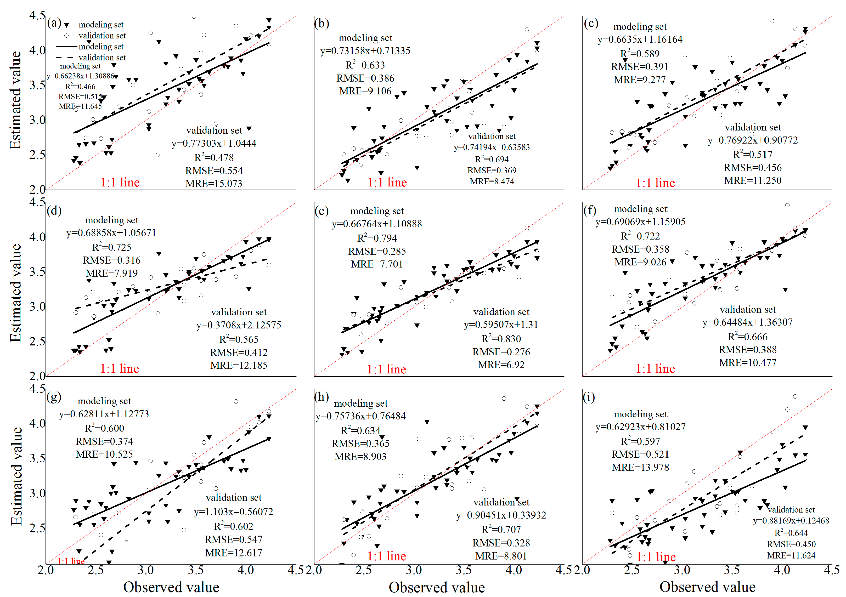
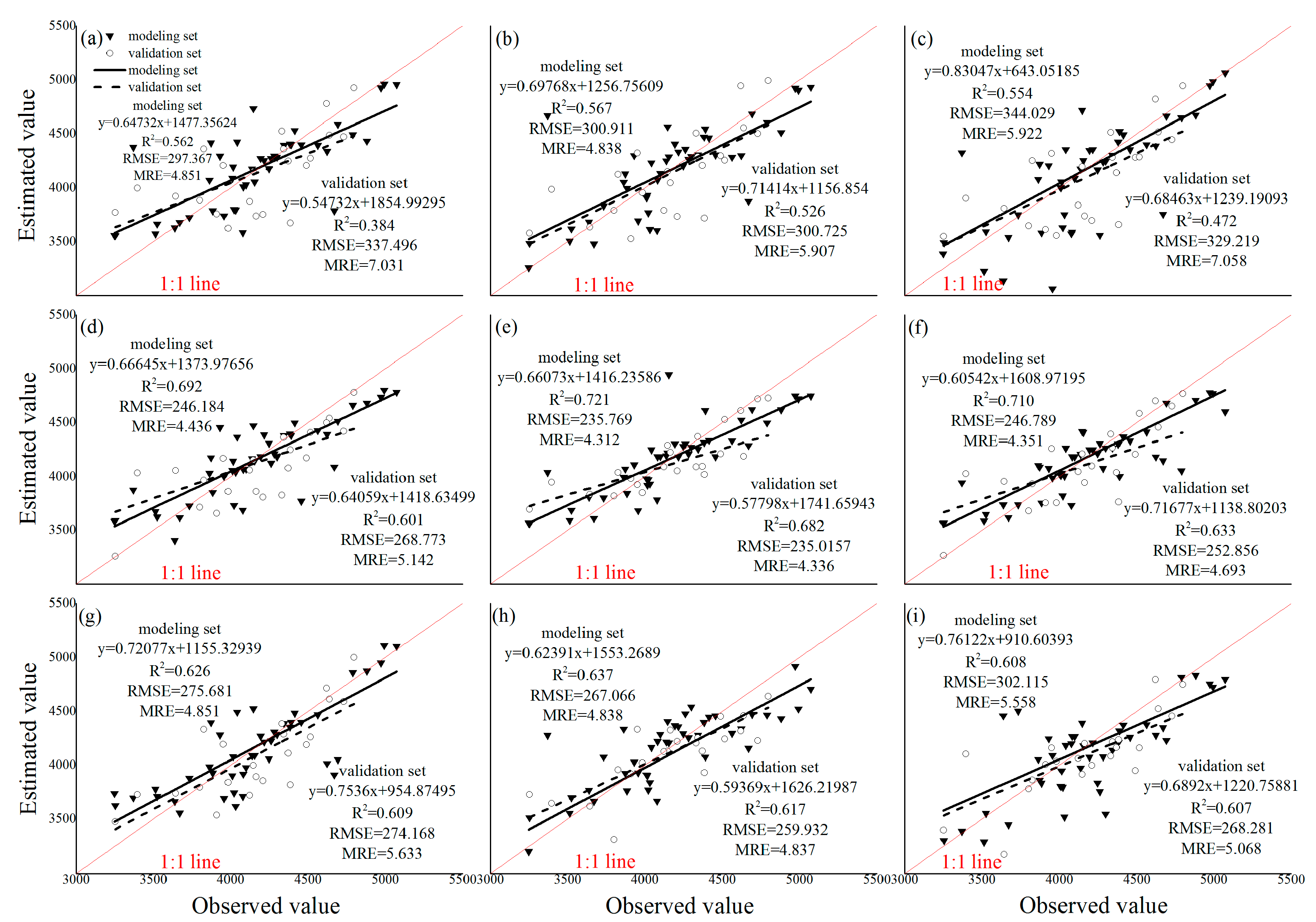
3.2. Establishment of LAI and Above-Ground Biomass Inversion Model Based on Optimal Spectral Index

The 14 groups of wavelength combinations were substituted into corresponding formulas for calculation, and the corresponding spectral index values were obtained. In the process of constructing the spectral indices with the best correlation coefficients with LAI, 14 spectral indices were divided into three groups as input variables to the model. The first set of variables consisted of the five spectral indices (DI, RI, NDVI, SAVI, and TVI) with the highest correlation coefficients with LAI calculated from the raw reflectance spectra, and was referred to as Combination 1; the second set of variables was calculated from the first-order differential reflectance spectrum of the five spectral indices with the highest correlation coefficient with LAI (FDDI, FDRI, FDNDVI, FDSAVI and FDTVI), and was referred to as Combination 2; the third group of variables was the highest 5 correlation coefficients among the 14 calculated spectral indices with LAI, consisting of FDDI, FDSAVI, NDVI, RI and TVI, and was referred to as Combination 3.

The process of constructing a spectral index with above-ground biomass is the same as the procedure for constructing a LAI spectral index. Therefore, the model input variables for estimating the above-ground dry matter were composed of Combination 1 (DI, RI, NDVI, SAVI, and TVI), Combination 2 (FDDI, FDSAVI, FDTVI, FDmNDI, and FDmSR) and Combination 3 (FDDI, FDSAVI, TVI, DI, and RI).

After the optimal spectral index combination of LAI and above-ground dry matter was established, SVM, RF and BPNN were used to model the two, respectively. The model results are shown in Figure 5 and Figure 6.

Table 5. Comparison of precision test results of estimation models.

	Model	Combination	Modeling Set R2	Validation Set R2	Modeling Set RMSE	Validation Set RMSE	Modeling Set MRE	Validation Set MRE
LAI	SVM	1	0.466	0.478	0.515	0.554	11.645	15.073
		2	0.633	0.694	0.386	0.369	9.106	8.474
		3	0.589	0.517	0.391	0.456	9.277	11.250
	RF	1	0.725	0.565	0.316	0.412	7.919	12.185
		2	0.794	0.830	0.285	0.276	7.701	6.920
		3	0.722	0.666	0.358	0.388	9.026	10.477
	BPNN	1	0.600	0.602	0.374	0.547	10.525	12.617
		2	0.634	0.707	0.365	0.328	8.903	8.801
		3	0.597	0.644	0.521	0.450	13.978	11.624
Above-ground biomass	SVM	1	0.562	0.384	301.367	337.496	4.851	7.031
		2	0.567	0.526	300.911	300.725	4.838	5.907
		3	0.554	0.472	344.029	329.219	5.922	7.058
	RF	1	0.692	0.601	246.184	268.773	4.436	5.142
		2	0.721	0.682	235.769	235.016	4.312	4.336
		3	0.710	0.633	246.789	252.856	4.351	4.693
	BPNN	1	0.626	0.609	275.681	274.168	4.851	5.633
		2	0.637	0.617	267.066	259.932	4.838	4.837
		3	0.608	0.607	302.115	268.281	5.558	5.068

shows the LAI and above-ground biomass estimation models of winter wheat with different combinations of input variables and modeling methods, as well as the prediction results of the validation set. An observation can be made that in the RF and BPNN models, the R² of the LAI and above-ground biomass estimation models’ modeling set and validation set were both higher than 0.6, indicating that the models had a good degree of linear fit accuracy and could be used to estimate the LAI and above-ground biomass of winter wheat. At the same time, a further observation can be made that under the same model, the R² of the modeling set and the validation set of Combination 2 in the LAI and above-ground biomass estimation models were higher than those of Combination 1 and Combination 3, and the RMSE and MRE were both lower. Under the same combination, the R² values of the RF model’s modeling set and validation set were higher than those of the SVM model and the BPNN model, and the RMSE and MRE were both lower. An observation can be made that Combination 2 was the optimal model input variable in the three modeling methods, indicating that the first-order differential spectral index contained more spectrally effective information related to LAI and above-ground biomass, and the predictive ability was higher for LAI and above-ground biomass. For the same input variable and different modeling methods, by comparing the model evaluation indicators, the order of accuracy of the models established by the three methods was: RF > BPNN > SVM. As such, the RF model was the best modeling method, which could extract the effective information of LAI and above-ground biomass to a greater extent. To summarize, the models established by the combination of the optimal input variables and the optimal modeling method for the LAI and above-ground biomass estimation models of winter wheat were the combination of input variable 2 and the RF model. The optimal winter wheat LAI estimation model was based on the combination of RF model and Combination 2. The R² of the optimal model modeling set was 0.794, that of the RMSE was 0.285, and that of the MRE was 7.701. Meanwhile, the R² of the validation set was 0.830, that of the RMSE was 0.276, and that of the MRE was 6.920. The optimal model for estimating the above-ground biomass of winter wheat was a model based on the combination of RF model and Combination 2. The R² of the optimal model modeling set was 0.721, that of the RMSE was 235.769, and that of the MRE was 4.312. At the same time, the R² of the validation set was 0.682, that of the RMSE was 235.016, and that of the MRE was 4.336. An observation can be made from the evaluation indicators in Table 5 that in the same spectral index combination and modeling method, the LAI estimation model based on winter wheat generally had higher accuracy than the above-ground biomass estimation model.

4. Discussion

In the calculation and selection process of spectral indices, all of the wavelength combinations of the indices were found to be in the red edge range and the optimal wavelength position is consistent with previous research results [12]. The red edge was the point where the reflectance of green plants increased the fastest between 670 and 760 nm. Studies have shown that the absorption spectrum curve of chlorophyll in leaves has a red edge, while the absorption spectrum curve of water and carotenoids does not have a red edge. As a result, the change and characteristic information of chlorophyll content can be reflected on the red edge to the greatest extent, because the red edge has a high sensitivity to chlorophyll content. In the present study, both LAI and above-ground biomass were found to be closely related to chlorophyll in leaves, because the growth of leaves requires chlorophyll to participate in photosynthesis. Such a factor is the fundamental reason for the growth of LAI and above-ground biomass. When selecting the optimal spectral index combination for modeling, the first-order differential spectral index was found to have a higher predictive ability for LAI and above-ground biomass. In analyzing the input characteristics of the model, an observation could be made that the first-order differential spectral index was closely related to LAI and above-ground biomass. The correlation of the first-order differential spectral index with LAI and above-ground biomass was better than that of the reflectance differential spectral index, the model constructed based on the first-order differential spectral index had stronger adaptability to unknown samples, and could improve the spectral response to LAI, above-ground biomass, and the ability of information mining, enhance the correlation between LAI, above-ground biomass, and spectra, and better characterize the growth status of winter wheat. Such findings could be attributed to the differential processing of canopy reflectance spectral data being able to reduce the influence of baseline drift and background noise, while enhancing the spectral characteristics of internal physiological and biochemical parameters of wheat. Notably, baseline drift and noise interference are mostly non-stationary signals. Hong [24] combined fractional order derivative and spectral variable selection, which could effectively eliminate the background noise [25] and improve the correlation between the spectra and LAI and above-ground biomass. In the present study, Combination 2 as input was found to be better than Combination 3 in predicting wheat LAI and above-ground biomass. Such findings could potentially be attributed to the combination of the original spectral reflectance and the first-order differential of the original spectral reflectance having a limited relationship with each other, resulting in a lower estimation accuracy than that of the same kind of spectral index. However, as input variables to predict wheat LAI and above-ground biomass, similar spectral indices may provide a better prediction, which is consistent with the findings of Liu et al. [12].

Among the three modeling methods selected in the present study, the estimation model based on RF for winter wheat LAI and above-ground biomass had the best accuracy, indicating that RF has more advantages than other models in retrieving winter wheat LAI and above-ground biomass. Such findings are basically consistent with the results of previous inversion of LAI of crops [26] and previous inversion of above-ground biomass of crops [27]. Previous studies have shown that the prediction accuracy of the estimation model was significantly affected by different modeling methods [28]. The results of the present study show that the prediction accuracy of SVM was lower than RF model. Such findings could be attributed to the core problem of SVM being to determine the kernel function and related parameters, and due to the limitation of parameter selection such as kernel function and penalty factor, the application thereof being restricted to a certain extent [29]. The model estimation accuracy of the BPNN model was low, which may be caused by the low generalization ability due to relatively few samples [30]. Meanwhile, RF is a machine learning method with integrated thinking, which has strong self-learning ability, strong tolerance to noise and outliers, and is not easy to overfit [31]. Therefore, RF can be used as the preferred method for monitoring and modeling of LAI and above-ground biomass of winter wheat and can better provide real-time and efficient technical services for future precision agriculture in practical applications. Additionally, under the same input combinations and modeling methods, the accuracy of the winter wheat LAI estimation model was found to be basically higher than that of the SPAD value estimation model. Such findings could be attributed to LAI being more intuitive than above-ground biomass. Morphological parameters and growth conditions were more easily identified, which is consistent with the findings of Lu et al. [15].

5. Conclusions

In this study, the extracted 14 spectral indices, which were calculated according to the optimal wavelength combination, had a strong correlation with winter wheat LAI and above-ground biomass. We compared and analyzed three groups of model input variables and the corresponding evaluation indicators from the modeling results. When the input variables were different, but the models were the same, Combination 2 provided the optimal model input variables. Combination 2 involved calculating the five spectral indices with the highest correlation coefficient to LAI and above-ground biomass using the reflection spectrum after first-order differential processing. However, when the modeling methods varied but the input variables were constant, the RF model was the optimal modeling method. By comprehensively comparing and analyzing the 18 model evaluation indicators of LAI and above-ground biomass, we established that the optimal winter wheat LAI estimation model was based on a combination of the RF model and Combination 2.

References

1. Chen, J.M.; Cihlar, J. Retrieving leaf area index of boreal conifer forests using Landsat TM images. Remote Sens. Environ. 1996, 55, 153–162. [Google Scholar] [CrossRef]
2. Sellers, P.J. Modeling the exchanges of energy, water, and carbon between continents and the atmosphere. Science 1997, 275, 502–509. [Google Scholar] [CrossRef] [Green Version]
3. Wu, F.; Li, Y.X.; Zhang, Y.Y.; Zhang, X.H.; Zou, X.C. Hyperspectral estimation of biomass of winter wheat at different growth stages based on machine learning algorithms. J. Triticeae Crops 2019, 39, 217–224, (In Chinese with English abstract). [Google Scholar] [CrossRef]
4. Zhang, L.X.; Chen, Y.Q.; Li, Y.X.; Ma, J.C.; Du, K.M.; Zheng, F.X.; Sun, Z.F. Estimating above ground biomass of winter wheat at early growth stages based on visual spectral. Spectrosc. Spect. Anal. 2019, 39, 2501–2506, (In Chinese with English abstract). [Google Scholar] [CrossRef]
5. Li, L.T.; Li, J.; Ming, J.; Wang, S.Q.; Ren, T.; Lu, J.W. Selection optimization of hyperspectral bandwidth and effective wavelength for predicting leaf area index in winter oilseed rape. Trans. Chin. Soc. Agric. Mach. 2018, 49, 156–165, (In Chinese with English abstract). [Google Scholar] [CrossRef]
6. Xie, Q.Y.; Huang, W.J.; Liang, D.; Peng, D.L.; Huang, L.S.; Song, X.Y.; Zhang, D.Y.; Yang, G.J. Research on universality of least squares support vector machine method for estimation leaf area index of winter wheat. Spectrosc. Spect. Anal. 2014, 34, 489–493, (In Chinese with English abstract). [Google Scholar] [CrossRef]
7. Zhang, J.J.; Cheng, T.; Guo, W.; Xu, X.; Ma, X.M.; Xie, Y.M.; Qiao, H.B. Leaf area index estimation model for UAV image hyperspectral data based on wavelength variable selection and machine learning methods. Plant Methods 2021, 17, 49. [Google Scholar] [CrossRef]
8. Oliveira, R.A.; Junior, J.M.; Costa, C.S.; Näsi, R.; Koivumäki, N.; Niemeläinen, O.; Kaivosoja, J.; Nyholm, L.; Pistori, H.; Honkavaara, E. Silage grass sward nitrogen concentration and dry matter yield estimation using deep regression and RGB images captured by UAV. Agronomy 2022, 12, 1352. [Google Scholar] [CrossRef]
9. Apolo-Apolo, O.E.; Pérez-Ruiz, M.; Martínez-Guanter, J.; Egea, G. A mixed data-based deep neural network to estimate leaf area index in wheat breeding trials. Agronomy 2020, 10, 175. [Google Scholar] [CrossRef] [Green Version]
10. Hama, A.; Tanaka, K.; Mochizuki, A.; Tsuruoka, Y.; Kondoh, A. Estimating the protein concentration in rice grain using UAV imagery together with agroclimatic data. Agronomy 2020, 10, 431. [Google Scholar] [CrossRef] [Green Version]
11. Tan, K.Z.; Wang, S.W.; Song, Y.Z.; Liu, Y.; Gong, Z.P. Estimating nitrogen status of rice canopy using hyperspectral reflectance combined with BPSO–SVR in cold region. Chemometr. Intell. Lab. 2017, 172, 68–79. [Google Scholar] [CrossRef]
12. Liu, S.; Yu, H.Y.; Zhang, J.H.; Zhou, H.G.; Kong, L.J.; Zhang, L.; Dang, J.M.; Sui, Y.Y. Study on Inversion Model of Chlorophyll Content in Soybean Leaf Based on Optimal Spectral Indices. Spectrosc. Spect. Anal. 2021, 41, 1912–1919, (In Chinese with English abstract). [Google Scholar] [CrossRef]
13. Bekele, F.; Korecha, D.; Negatu, L. Influence of rainfall features on barley yield in Sinana district of Ethiopia. J. Agrometeorol. 2017, 19, 125–128. [Google Scholar] [CrossRef]
14. Kuusk, A. Specular reflection in the signal of LAI–2000 plant canopy analyzer. Agr. Forest. Meteorol. 2016, 221, 242–247. [Google Scholar] [CrossRef]
15. Lu, J.S.; Chen, S.M.; Huang, W.M.; Hu, T.T. Estimating of aboveground biomass and leaf area index of summer maize using SEPLS_ELM model. Trans. Chin. Soc. Agric. Eng. 2021, 37, 128–135, (In Chinese with English abstract). [Google Scholar] [CrossRef]
16. Cortes, C.; Vapnik, V. Support–vector networks. Mach. Learn. 1995, 20, 273–297. [Google Scholar] [CrossRef]
17. Breiman, L. Random forest. Mach. Learn. 2001, 45, 5–32. [Google Scholar] [CrossRef] [Green Version]
18. Hecht–Nielsen, R. Theory of the backpropagation neural network. Neural Netw. 1988, 1, 445. [Google Scholar] [CrossRef]
19. Chen, Y.; Wang, L.; Bai, Y.L.; Lu, Y.L.; Ni, L.; Wang, Y.H.; Xu, M.Z. Quantitative relationship between effective accumulated temperature and summer maize plant height and leaf area index under different nitrogen, phosphorus and potassium treatments. Chin. Agric. Sci. 2021, 54, 4761–4777, (In Chinese with English abstract). [Google Scholar] [CrossRef]
20. Li, Y.Y.; Chang, Q.R.; Liu, X.Y.; Yan, L.; Luo, D.; Wang, S. Remote sensing estimation of SPAD value of maize leaves based on hyperspectral and BP neural network. Trans. Chin. Soc. Agric. Eng. 2016, 32, 135–142, (In Chinese with English abstract). [Google Scholar] [CrossRef]
21. Kira, O.; Nguy–Robertson, A.L.; Arkebauer, T.J.; Linker, R.; Gitelson, A.A. Informative spectral bands for remote green LAI estimation in C3 and C4 crops. Agr. Forest. Meteorol. 2016, 218–219, 243–249. [Google Scholar] [CrossRef] [Green Version]
22. Ancona, N.; Maglietta, R.; Stella, E. Data representations and generalization error in kernel based learning machines. Pattern Recognit. 2006, 39, 1588–1603. [Google Scholar] [CrossRef]
23. Chen, J.Y.; Wang, X.T.; Zhang, Z.T.; Han, J.; Yao, Z.H.; Wei, G.F. Soil salinization monitoring method based on uav-satellite remote sensing scale-up. Trans. Chin. Soc. Agric. Mach. 2019, 50, 161–169, (In Chinese with English abstract). [Google Scholar] [CrossRef]
24. Hong, Y.S.; Liu, Y.L.; Chen, Y.Y.; Liu, Y.F.; Yu, L.; Liu, Y.; Cheng, H. Application of fractional–order derivative in the quantitative estimation of soil organic matter content through visible and near–infrared spectroscopy. Geoderma 2018, 337, 758–769. [Google Scholar] [CrossRef]
25. Zhang, Y.K.; Luo, B.; Pan, D.Y.; Song, P.; Lu, W.C.; Wang, C.; Zhao, C.J. Estimation of Canopy Nitrogen Content of Soybean Crops Based on Fractional Differential Algorithm. Spectrosc. Spect. Anal. 2018, 38, 3221–3230, (In Chinese with English abstract). [Google Scholar] [CrossRef]
26. Zhang, Y.M.; Ta, N.; Guo, S.; Chen, Q.; Zhao, L.C.; Li, F.L.; Chang, Q.R. Combining spectral and textural information from UAV RGB images for leaf area index monitoring in kiwifruit orchard. Remote Sens. 2022, 14, 1063. [Google Scholar] [CrossRef]
27. Wang, F.L.; Yang, M.; Ma, L.F.; Zhang, T.; Qin, W.L.; Li, W.; Zhang, Y.H.; Sun, Z.C.; Wang, Z.M.; Li, F.; et al. Estimation of above-ground biomass of winter wheat based on consumer-grade multi-spectral UAV. Remote Sens. 2022, 14, 1251. [Google Scholar] [CrossRef]
28. Xia, T.; Wu, W.B.; Zhou, Q.B.; Zhou, Y. Comparison of two inversion methods for winter wheat leaf area index based on hyperspectral remote sensing. Trans. Chin. Soc. Agric. Eng. 2013, 29, 139–147, (In Chinese with English abstract). [Google Scholar] [CrossRef]
29. Azarmdel, H.; Jahanbakhshi, A.; Mohtasebi, S.S.; Muñozc, A.R. Evaluation of image processing technique as an expert system in mulberry fruit grading based on ripeness level using artificial neural networks (ANNs) and support vector machine (SVM). Postharvest Biol. Technol. 2020, 166, 111201. [Google Scholar] [CrossRef]
30. Zhang, Y.; Zhou, M.R. Application of Artificial Neural Network BP Algorithm in Near Infrared Spectroscopy. Infrared 2006, 27, 1–4, (In Chinese with English abstract). [Google Scholar] [CrossRef]
31. Fu, Z.P.; Jiang, J.; Gao, Y.; Krienke, B.; Wang, M.; Zhong, K.T.; Cao, Q.; Tian, Y.C.; Zhu, Y.; Cao, W.X.; et al. Wheat Growth Monitoring and Yield Estimation based on Multi-Rotor Unmanned Aerial Vehicle. Remote Sens. 2020, 12, 508. [Google Scholar] [CrossRef] [Green Version]
Figure 1. Aerial photograph of winter wheat research area and some sampling plots in Yangling, Shaanxi.
Agronomy 12 01729 g001
Figure 2. Diagrams of architectures used in the experiments.
Agronomy 12 01729 g002
Figure 3. Correlation matrix diagram of spectral indices and leaf area index(LAI). (a) DI and LAI; (b) FDDI and LAI; (c) RI and LAI; (d) FDRI and LAI; (e) NDVI and LAI; (f) FDNDVI and LAI; (g) SAVI and LAI; (h) FDSAVI and LAI; (i) TVI and LAI; (j) FDTVI and LAI; (k) mSR and LAI; (l) FDmSR and LAI; (m) mNDI and LAI; (n) FDmNDI and LAI.
Agronomy 12 01729 g003aAgronomy 12 01729 g003b
Figure 4. Correlation matrix diagram of spectral indices and above-ground biomass. (a) DI and above-ground biomass; (b) FDDI and above-ground biomass; (c) RI and above-ground biomass; (d) FDRI and above-ground biomass; (e) NDVI and above-ground biomass; (f) FDNDVI and above-ground biomass; (g) SAVI and above-ground biomass; (h) FDSAVI and above-ground biomass; (i) TVI and above-ground biomass; (j) FDTVI and above-ground biomass; (k) mSR and above-ground biomass; (l) FDmSR and above-ground biomass; (m) mNDI and above-ground biomass; (n) FDmNDI and above-ground biomass.
Agronomy 12 01729 g004aAgronomy 12 01729 g004b
Figure 5. Prediction results of modeling set and validation set of winter wheat leaf area index inversion model with different input variables and modeling methods. (a) SVM Model input variable is combination 1; (b) SVM Model input variable is combination 2; (c) SVM Model input variable is combination 3; (d) RF Model input variable is combination 1; (e) RF Model input variable is combination 2; (f) RF Model input variable is combination 3; (g) BPNN Model input variable is combination 1; (h) BPNN Model input variable is combination 2; (i) BPNN Model input variable is combination 3.
Agronomy 12 01729 g005
Figure 6. Prediction results of modeling set and validation set of winter wheat above-ground biomass inversion model with different input variables and modeling methods (a) SVM Model input variable is combination 1; (b) SVM Model input variable is combination 2; (c) SVM Model input variable is combination 3; (d) RF Model input variable is combination 1; (e) RF Model input variable is combination 2; (f) RF Model input variable is combination 3; (g) BPNN Model input variable is combination 1; (h) BPNN Model input variable is combination 2; (i) BPNN Model input variable is combination 3.
Agronomy 12 01729 g006