Solar Radiation Prediction Model for the Yellow River Basin with Deep Learning

Abstract

Solar radiation is the main source of energy on the Earth’s surface. It is very important for the environment and ecology, water cycle and crop growth. Therefore, it is very important to obtain accurate solar radiation data. In this study, we use the highest temperature T_max, lowest temperature T_min, average temperature T_avg, wind speed U, relative humidity RH, sunshine duration H and maximum sunshine duration H_max as input variables to construct a deep learning prediction model of solar radiation in the Yellow River Basin. It is compared with the recommended and corrected values of the widely used Å-P method. The results show that: (1) The correction results of the Å-P equation are better in the upstream and downstream of the Yellow River Basin but worse in the midstream. (2) The prediction result of the deep learning model in the Yellow River Basin is far better than that of the Å-P equation using the FAO-56 recommended value. It is the best in the downstream of the Yellow River Basin: R² increases from 0.894 to 0.934; MSE, RMSE and MAE decrease by 43.12%, 27.73% and 25.80%, respectively. The upstream prediction result comes in second: R² increases from 0.888 to 0.921; MSE, RMSE and MAE decrease by 33.27%, 20.02% and 19.04%, respectively. The midstream result is the worst: R² increases from 0.869 to 0.874; MSE, RMSE and MAE decrease by −0.50%, 0.07% and 3.82%, respectively. (3) The prediction results of the deep learning model in the upstream and downstream of the Yellow River Basin are far better than those of the Å-P equation using correction. The R² in the upstream of the Yellow River Basin increases from 0.889 to 0.921. MSE, RMSE and MAE decrease by 22.11%, 11.84% and 8.94%, respectively. R² in the downstream of the Yellow River Basin increases from 0.900 to 0.934, and MSE, RMSE and MAE decrease by 13.21%, 11.40% and 5.55%, respectively. In the midstream of the Yellow River Basin, the prediction results of the deep learning model are worse than those of the Å-P equation using correction: R² increases from 0.870 to 0.874, but MSE, RMSE and MAE decrease by −24.93%, −10.83% and −11.56%, respectively.

1. Introduction

Solar radiation is not only the most basic energy source on Earth but is also an important driving factor of various physical, chemical and biological processes in the natural environment. It has a wide range of applications in many aspects, such as the infrastructure and construction industry, atmospheric physics and the practical utilization of renewable energy [1,2], the estimation of reference crop evapotranspiration [3], evapotranspiration simulation in hydrology [4], photovoltaic power generation [5,6], etc. Therefore, it is particularly important to obtain accurate solar radiation data.

Despite the wide range of applications of solar radiation data, there are few radiation stations for the routine observation of solar radiation in our country. According to statistics, in China, only about 4% of the national ground meteorological observation networks can measure solar radiation. Moreover, solar radiation is usually measured at a specific location through a variety of instruments. The cost of these instruments, including measurement and maintenance costs, is high, Therefore, compared with other meteorological factors such as rainfall, sunshine and wind speed, the data of solar radiation are relatively scarce. The scarcity of solar radiation measurement requires people to adopt corresponding methods to estimate it and obtain more accurate solar radiation data in a finer spatial distribution. Over the years, scholars at home and abroad have done a lot of research on the estimation of solar radiation and have successively put forward some methods. Among them, the Ångström-Prescott equation based on sunshine (hereinafter referred to as the Å-P equation) has been proved to be the best in many studies [7,8,9,10]. FAO irrigation and drainage Document No. 56 (hereinafter referred to as FAO-56) recommends the Å-P equation to estimate solar radiation in the absence of measured solar radiation data or low-quality solar radiation data and recommends the parameters of a = 0.25 and b = 0.50.

Although the Å-P equation performs well and is widely used, due to the influence of climate and geographical location factors in different regions, the FAO-56 recommended values in different regions are different. Therefore, the application of the Å-P equation in different regions is usually limited by the lack of corrected parameters. To solve the limitations of the Å-P equation, we need to develop more accurate methods to predict solar radiation.

In recent years, with the rapid development of artificial intelligence and neural networks, many machine learning models, such as artificial neural networks, support vector machines and random forest, have been successfully applied to the prediction of solar radiation: Alawi et al. [11], Mohandas et al. [12], Reddy et al. [13] and Yildiz et al. [14] in Oman, Saudi Arabia used artificial neural networks to estimate solar radiation in India and Turkey; Chen et al. [15] used the data of three meteorological stations in Liaoning Province to establish seven support vector machine models with different input attributes and evaluate them and five empirical models based on sunshine; Ibrahim and Khatib [16] proposed a hybrid hourly solar radiation prediction model based on random forest technology and the firefly algorithm and compare it with the traditional artificial neural network model, the traditional random forest model and an artificial neural network model optimized by the firefly algorithm. The above research results show that machine learning models can predict solar radiation.

Deep learning is similar to artificial neural networks and belongs to the field of machine learning, but it has a deeper neural network, which means that deep learning has a stronger learning ability and needs larger data sets to improve its prediction performance. Nowadays, deep learning has become more and more mature in the field of computer vision. Remarkable achievements have been MAEe in the fields of perception, speech recognition and natural language processing. Deep learning models have been successfully applied to predict the reference crop evapotranspiration ET₀ [17,18], but there is little literature related to the deep learning model in predicting solar radiation.

Therefore, based on the measured meteorological data of 28 stations in the Yellow River Basin for many years, this study establishes a deep learning model for predicting solar radiation in the Yellow River Basin in China. There are three main purposes: (1) Based on the measured solar radiation data of 28 stations in the Yellow River Basin for many years, we want to correct the parameters of the traditional Å-P equation and analyze the correction results through the evaluation metrics; (2) We want to develop and establish a DL model for accurately predicting solar radiation in the Yellow River Basin by using widely available input variables; (3) By comparing the DL model with the recommended and corrected values of Å-P parameters, the feasibility of the DL model replacing the Å-P equation to predict solar radiation in the Yellow River Basin is studied.

2. Materials and Methods

2.1. Study Location and Data

In this study, we select 28 stations with measured daily solar radiation long-term data in 9 provinces and regions in the Yellow River Basin. All of these stations are located in or near the Yellow River Basin. The detailed geographical information of each station is shown in

Table 1. Basic information of stations in the Yellow River Basin.

Site Name	Longitude	Latitude	Altitude	Average Temperature	Province	Data Period
Yushu	97.02	33.02	3681.2	3.59	Qinghai	1960–2016
Guoluo	100.25	34.47	3719	0.04	Qinghai	1993–2016
Gangcha	100.13	37.33	3301.5	0.05	Qinghai	1993–2016
Geermu	94.9	36.42	2807.7	5.75	Qinghai	1957–2016
Xining	101.77	36.62	2261.2	6.09	Qinghai	1959–2016
Ganzi	100	31.62	3393.5	5.98	Sichuan	1994–2016
Hongyuan	102.55	32.8	3491.6	1.75	Sichuan	1994–2016
Wuwei	102.67	37.92	1530.9	8.54	Gansu	1961–2016
Minqin	103.08	38.63	1367	8.78	Gansu	1957–2016
Yuzhong	104.15	35.87	1874.1	6.99	Gansu	2005–2016
Guyuan	106.27	36	1752.2	6.95	Ningxia	1985–2016
Yinchuan	106.22	38.48	1111.4	9.51	Ningxia	1959–2016
Huhehaote	111.68	40.82	1063	7.13	Neimenggu	1959–2016
Erlianhaote	111.97	43.65	964.7	4.56	Neimenggu	1957–2016
Wulatezhongqi	108.52	41.57	1288.2	5.73	Neimenggu	1992–2016
Dongsheng	109.98	39.83	1460.4	6.67	Neimenggu	1992–2016
Taiyuan	112.55	37.78	777.9	10.38	Shanxi	1959–2016
Datong	113.33	40.1	1067.2	7.21	Shanxi	1960–2016
Houma	111.37	35.65	433.7	13.04	Shanxi	1959–2016
Yanan	109.5	36.6	957.8	10.21	Shanxi	1990–2016
Jinghe	108.97	34.43	410	14.90	Shanxi	2006–2016
Ankang	109.03	32.72	290.8	15.86	Shanxi	1990–2016
Nanyang	112.58	33.03	129.2	15.22	Henan	1990–2016
Zhengzhou	113.65	34.72	110.4	14.84	Shanxi	1957–2016
Anyang	114.37	36.12	75.5	14.15	Shanxi	1960–2016
Fushan	121.25	37.5	32.6	12.77	Shandong	1992–2016
Jinan	116.98	36.68	51.6	14.77	Shandong	1959–2016
Juxian	118.83	35.58	107.4	12.66	Shandong	1990–2016

. The Yellow River Basin covers an area of 795,000 square kilometers, with latitude ranging from 26.58° N to 49.22° N, longitude ranging from 94.68° E to 122.27° E and altitude ranging from 32.6 m to 3719.0 m. The basin is characterized by water shortage, serious water and soil loss and high sediment content. Since the 1990s, it has become more frequent that river water cannot enter the sea. China attaches great importance to the sustainable utilization of water resources in this basin. However, the information about the coefficients of the Å-P equation in this basin is very limited. In addition, even for the same site, the coefficients of Å-P equations given by different researchers often vary greatly, which causes confusion and difficulties in the application of the model [19].

Due to various factors, such as the influence of solar radiation and sunshine time observation data in different degrees, there are missing data and exceptions. To avoid missing values and the effects of outliers, before the statistical analysis of data, we apply the following preprocessing:

(1)

If one or all of the measured meteorological data on a day is missing, the data of that day shall be deleted;

(2)

If Rs/Ra or n/N is greater than 1, we delete the data of that day to ensure that the data has real physical meaning (where Rs and Ra are global and extraterrestrial solar radiation (MJ/(M² · d)), respectively; n represents the actual sunshine hours in a day; N represents the maximum sunshine hours on the same day);

(3)

If there are more than 10 missing data in a month, the data of that month will be deleted.

The corrected values of the Å-P equation of each station are fitted by the least square error method, and the data of each station are grouped by years. The first 3/4 of the data is used as the training data set to fit the corrected values of the Å-P equation, and the remaining 1/4 of the data is used as the test data set to verify the corrected values of the Å-P equation. R², RMSE, RE, MAE and d evaluate its performance. The DL model selects the highest temperature T_max, lowest temperature T_min, average temperature T_avg, wind speed U, relative humidity RH, sunshine duration H and maximum sunshine duration H_max as input values and selects 70% of the data set as the training set, 15% as the verification set and 15% as the prediction set. The training set is used to train the model. The validation set is used to evaluate the performance of the model and calculate the evaluation metrics. The prediction set is used to evaluate the generalization and prediction ability of the model. The training set, validation set and prediction set are selected independently without repetition.

2.2. Ångström-Prescott Equation

The Å-P equation was originally a simple linear equation proposed by Angstrom [20] in 1924. In essence, it is a linear function relationship between the ratio of daily total irradiance to daily clear sky radiation on the horizontal plane and the ratio of daily average sunshine hours to maximum possible sunshine hours. The parameters of the equation are determined by Stockholm data. To solve the difficulty of obtaining clear sky radiation data, Prescott [21] suggested using extraterrestrial radiation to replace it in 1940, which finally promoted the formation of the Å-P equation.

To commemorate the great contributions MAEe by Ångström and Prescott to the estimation of solar radiation, later generations call the relationship between the sunny index and relative sunshine (or other meteorological parameters) the Ångström-Prescott equation. The basic form of the equation represents the simple linear relationship between the sunny index and relative sunshine:

$$\frac{Rs}{Ra}=a+b\frac{n}{N}$$

(1)

where Rs and Ra are global and extraterrestrial solar radiation (MJ/(M² · d)), respectively; a and b are empirical coefficients between 0 and 1 and their sum is clear sky transmittance; n represents the actual sunshine hours in a day; N represents the maximum sunshine hours on the same day.

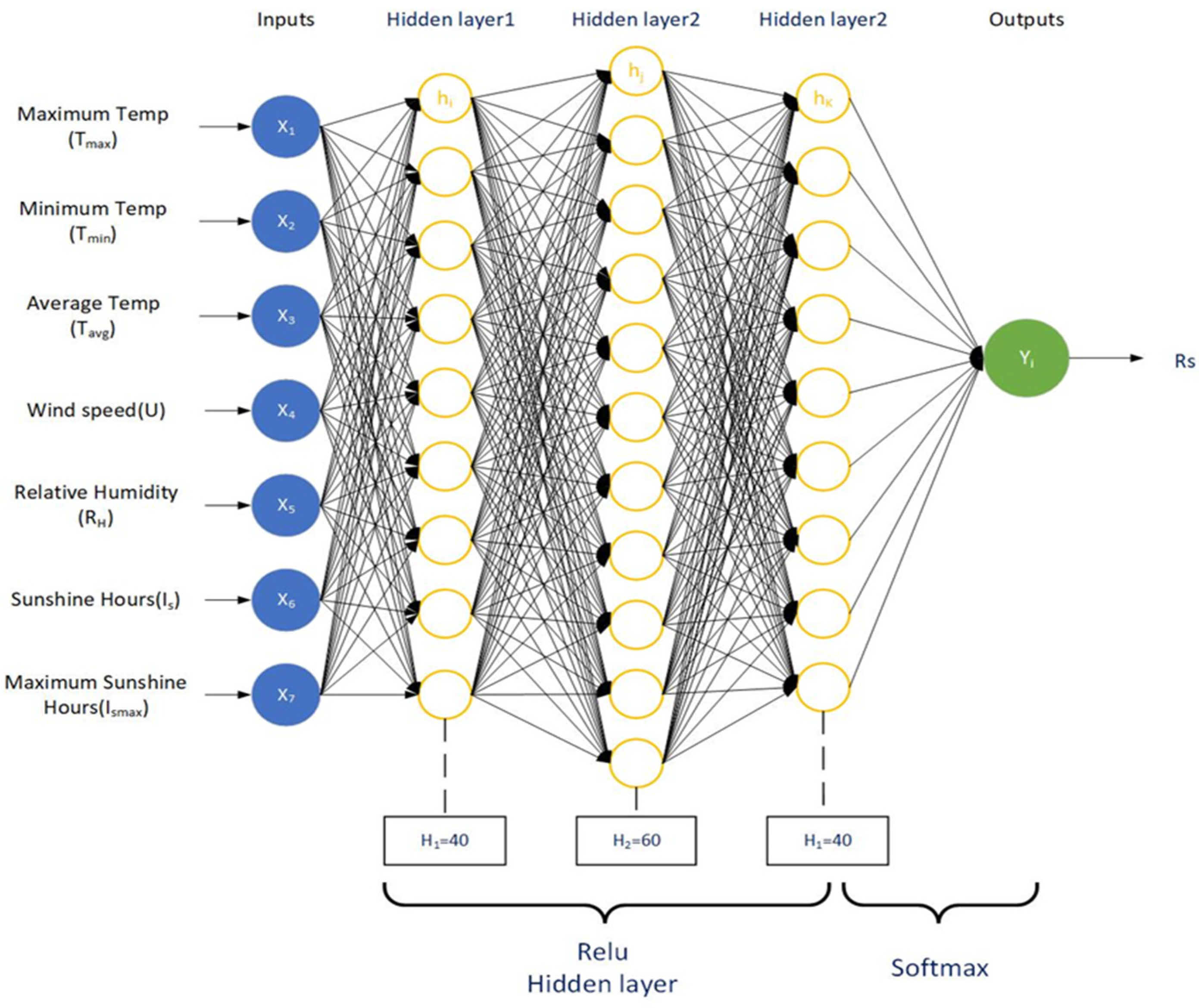
2.3. Deeping Learning Model

The earliest neural network originated from the neuron model proposed by McCulloch and Pitts in 1943. In 1986, Rumelhart and McClelland [22] invented the back-propagation (BP) algorithm. In 2006, Hinton et al. [23] formally proposed the concept of deep learning. In this paper, a method of using deep learning to predict solar radiation is proposed. By considering multiple hidden layers, different numbers of neurons in hidden layers and the modified linear function ReLU, a multi-layer DL model is established. In addition, our model is optimized by the stochastic gradient descent method. Figure 1 shows the framework of the deep learning model.

The research shows that selecting appropriate input parameters is very important for a more accurate prediction of solar radiation. In this paper, through multiple tests on the number of prediction model layers and neurons, the optimal number of hidden layers and the optimal number of hidden neurons are finally determined, which are 40 neurons in the first hidden layer, 60 neurons in the second hidden layer and 40 neurons in the third hidden layer, respectively. In addition, the modified linear function ReLU is selected as the activation function, because its calculation is simple and fast and the convergence rate of the stochastic gradient descent (SGD) optimization algorithm for the ReLU function is faster than others. Therefore, this paper establishes a DL model with three hidden layers (40 60 40) and a ReLU function as the activation function.

The ReLU function is given by the following equation:

$$f\left(x\right)=max\left(0,x\right)$$

(2)

The derivative of the ReLU function is:

$$f^{\prime }\left(x\right)=\left\{\begin{array}{cc}1,& if x>0\\ 0,& otherwise\end{array}\right.$$

(3)

The cross-entropy loss function J is:

$$J\left(W,B\right)=-\frac{1}{N}{\displaystyle \sum }_{i=1}^N{\displaystyle \sum }_{j=1}^k{y}_j^{\left(i\right)}log{\widehat{y}}_j^{\left(i\right)}$$

(4)

The learning process of the DL model consists of forward-propagation and back-propagation. During forward-propagation, the input values go through the input layer, the hidden layer and the output layer. If the output layer does not get the desired output, the back-propagation is carried out. The stochastic gradient descent method back-propagates the error along the original channel and modifies the weight of each neuron in the hidden layer. Thus, the output error is minimized.

$$Z^{\left[1\right]}=Relu\left({\displaystyle \sum }_{i=1}^n\left(x_i\ast w_1\right)+b_1\right)$$

(5)

$$Z^{\left[2\right]}=Relu\left({\displaystyle \sum }_{j=1}^n\left(h_j\ast w_2\right)+b_2\right)$$

(6)

$$Z^{\left[3\right]}=Relu\left({\displaystyle \sum }_{k=1}^n\left(h_k\ast w_3\right)+b_3\right)$$

(7)

$$Z^{\left[4\right]}=Softmax\left({\displaystyle \sum }_{L=1}^n\left(h_L\ast w_4\right)+b_4\right)$$

(8)

$$Y=Softmax\left(x_k\right)=\frac{exp\left(x_k\right)}{{{\displaystyle \sum }}_{k=1}^{n}exp(x_k)}$$

(9)

$$w_1=w_1-\alpha \frac{\partial J}{\partial W_1}$$

(10)

$$b_1=b_1-\alpha \frac{\partial J}{\partial b_1}$$

(11)

Figure 1 presents a DL structure composed of an input layer, three hidden layers and a final output layer; Y is the output of the output layer; x_i is the input layer input; w₁, w₂, w₃ and w₄ are the weight matrices connecting layers; b₁, b₂, b₃ and b₄ are the bias terms of hidden neurons for each hidden layer. Equations (10) and (11) denote the stochastic gradient descent method in back-propagation, w₁ $\in$ w, b₁ $\in$ b.

2.4. Model Evaluation Metrics

The metrics to evaluate the performance of the model include the determination coefficient R², mean square error MSE, rooted mean square error RMSE, mean absolute error MAE, relative error RE and consistency index d. Their calculation equations are as follows:

$$R^2=\frac{{\left[{{\displaystyle \sum }}_{i=1}^m\left(p_i-\overline{p}\right)\left(o_i-\overline{o}\right)\right]}^2}{{{\displaystyle \sum }}_{i=1}^m{\left(p_i-\overline{p}\right)}^2{{\displaystyle \sum }}_{i=1}^n{\left(0_i-\overline{0}\right)}^2}$$

(12)

$$\mathrm{MSE}=\frac{1}{m}{\displaystyle \sum }_1^m{(y_i-\overline{y_i})}^2$$

(13)

$$\mathrm{RE}=\sqrt{\frac{1}{m}{\displaystyle \sum }_1^m{(y_i-\overline{y_i})}^2}$$

(14)

$$\mathrm{MAE}=\frac{1}{m}{\displaystyle \sum }_1^m\left|y_i-\overline{y_i}\right|$$

(15)

$$\mathrm{RE}=\frac{\mathrm{RMSE}}{\overline{o}}$$

(16)

$$d=1-\frac{{{\displaystyle \sum }}_{i=1}^n{(p_i-o_i)}^2}{{{\displaystyle \sum }}_{i=1}^n{\left(\left|\left.p_i-\overline{o}\right|+\left|\left.o_i-\overline{o}\right|\right.\right.\right)}^2}$$

(17)

where O_i is the i-th observation data (MJ/(M²·d); P_i is the i-th prediction data (MJ/(M²·d); $\overline{O}$ is the average value of the observation data group (MJ/(M²·d); $\overline{P}$ is the average value of the prediction data group (MJ/(M²·d); $y_i-\overline{y_i}$ is the difference between the i-th prediction values and the measured values (MJ/(M²·d), i = 1, 2, …, m; m is the number of statistical samples.

Among them, the lower the values of MSE, RMSE and MAE, the better the performance of the model. The determination coefficient R² reflects the fitting degree between the measured and predicted solar radiation values of the station. When the determination coefficient R² > 0.80, RE < 0.20 and d ≥ 0.95, the prediction effect of the model is better.

3. Results

3.1. Corrected Å-P Parameters and Performance Evaluation

The corrected values of the Å-P equation of each station are fitted by the least square error method, and the data of each station are grouped by years. The first 3/4 of the data is used as the training data set to fit the corrected values of the Å-P equation, and the remaining 1/4 of the data is used as the test data set to verify the corrected values of the Å-P equation. R², RMSE, RE, MAE and d evaluate its performance.

Table 2. Å-P parameter calibration and performance evaluation of each station.

Watershed Distribution	Site Name	Province	a	b	R2	RMSE	RE	MAE	d
Upstream	Yushu	Qinghai	0.20	0.61	0.74	3.309	0.20	2.265	0.93
Upstream	Guoluo	Qinghai	0.25	0.58	0.87	2.451	0.14	1.835	0.96
Upstream	Gangcha	Qinghai	0.20	0.62	0.93	1.705	0.10	1.269	0.98
Upstream	Geermu	Qinghai	0.26	0.57	0.96	1.518	0.08	1.106	0.99
Upstream	Xining	Qinghai	0.18	0.61	0.92	1.896	0.12	1.399	0.98
Upstream	Ganzi	Sichuan	0.29	0.54	0.88	2.127	0.11	1.630	0.96
Upstream	Hongyuan	Sichuan	0.18	0.68	0.81	3.766	0.24	2.763	0.93
Upstream	Wuwei	Gansu	0.13	0.69	0.89	2.960	0.16	2.290	0.97
Upstream	Minqin	Gansu	0.20	0.53	0.95	1.595	0.09	1.168	0.99
Upstream	Yuzhong	Gansu	0.17	0.58	0.95	2.027	0.13	1.692	0.98
Upstream	Guyuan	Ningxia	0.16	0.61	0.93	2.028	0.14	1.528	0.98
Upstream	Yinchuan	Ningxia	0.20	0.57	0.93	2.023	0.13	1.435	0.98
Upstream	Huhehaote	Neimenggu	0.18	0.61	0.91	2.142	0.13	1.522	0.98
Upstream	Erlianhaote	Neimenggu	0.20	0.60	0.93	2.236	0.13	1.658	0.98
Upstream	Wulatezhongqi	Neimenggu	0.23	0.55	0.94	2.011	0.12	1.459	0.98
Upstream	Dongsheng	Neimenggu	0.16	0.58	0.93	2.542	0.17	1.707	0.97
Midstream	Taiyuan	Shanxi	0.16	0.59	0.86	2.823	0.20	2.122	0.96
Midstream	Datong	Shanxi	0.17	0.60	0.92	2.119	0.14	1.610	0.98
Midstream	Houma	Shanxi	0.16	0.58	0.86	2.664	0.22	1.981	0.96
Midstream	Yanan	Shanxi	0.14	0.58	0.82	3.296	0.24	2.340	0.95
Midstream	Jinghe	Shanxi	0.19	0.50	0.87	3.739	0.29	2.988	0.94
Midstream	Ankang	Shanxi	0.16	0.54	0.88	2.621	0.23	1.883	0.97
Midstream	Nanyang	Henan	0.19	0.53	0.86	2.748	0.23	2.070	0.96
Downstream	Zhengzhou	Shanxi	0.17	0.55	0.89	2.594	0.22	1.983	0.96
Downstream	Anyang	Shanxi	0.16	0.52	0.85	2.657	0.21	2.025	0.96
Downstream	Fushan	Shandong	0.16	0.56	0.95	1.736	0.12	1.323	0.98
Downstream	Jinan	Shandong	0.11	0.60	0.88	2.759	0.23	2.039	0.96
Downstream	Juxian	Shandong	0.21	0.53	0.94	1.715	0.12	1.289	0.98

shows the corrected values of the Å-P parameters and their performance evaluation of each station.

It can be seen from Table 2 that the values of a range from 0.11 to 0.29 and the values of b range from 0.50 to 0.69. The trend of coefficient a is that the average altitudes and longitudes of the upstream, midstream and downstream of the Yellow River Basin are (2191.73 m, 103.82°), (656.23 m, 111.37°) and (75.5 m, 117.02°), respectively. The maximum value of coefficient a is 0.29, which appears in Ganzi, Sichuan Province, with altitude and longitude of 3393.5 m and 100°, respectively. The minimum value is 0.11. It appears in Jinan, Shandong Province, with altitude and longitude of 51.6 m and 116.98°, respectively. The trend of coefficient b is opposite to that of coefficient a. In the upstream of the Yellow River Basin, the values of coefficient b are higher, with an average value of 0.60, and in the midstream and downstream of the Yellow River Basin, the values of coefficient b are lower, with average values of 0.56 and 0.55. The relationship between coefficient b and altitude is similar to that of coefficient a and tends to increase with the increase in altitude, but the relationship between coefficient b and longitude is opposite to that of coefficient a and tends to increase with the increase in longitude. The maximum value of b is 0.69, which appears in Wuwei, Gansu Province, with altitude and longitude of 1530.9 m and 102.67°, respectively. The minimum value of b is 0.50, which appears in Jinghe River, Shanxi Province, with altitude and longitude of 410 m and 108.97°, respectively.

It can be seen from the evaluation metrics that the corrected Å-P parameters have a good prediction effect. The average value of R² of 28 stations in the Yellow River Basin is 0.89, the maximum value is 0.96 at Golmud station and the minimum value is 0.74 at Yushu station. Except for Yushu station in Qinghai Province, the R² values of the other 27 stations are greater than 0.80, and the R² values of 14 stations are greater than 0.90. The average values of RMSE, MAE, RE and d of all stations are 2.422, 0.17, 1.799 and 0.97, the maximum values are 3.739, 0.29, 2 and 0.94 and the minimum values are 1.518, 0.08, 1.106 and 0.99, respectively. The RMSE values of 6 stations are less than 2.00, those of 18 stations are between 2.00 and 3.00 and those of 4 stations are greater than 3.00. The maximum value is 3.739 at Shanxi Jinghe station. The MAE values of 19 stations are within 2.00, those of 9 stations are between 2.00 and 3.00 and the maximum value is 2.988 at Jinghe River in Shanxi Province. The RE values of 2 stations are less than 0.1, those of 17 stations are between 0.1 and 0.2 and those of 9 stations are between 0.2 and 0.3. The maximum value is 0.29 at Jinghe River station, Shanxi Province. In terms of the d values, only 3 stations are between 0.91 and 0.95 and the remaining 25 stations’ d values are between 0.95 and 0.99, with the maximum values of 0.99 at Golmud in Qinghai Province. In general, the Golmud station in Qinghai Province has the best correction effect, and the Jinghe station in Shanxi Province has the worst correction effect.

From the results of the upstream, midstream and downstream of the Yellow River Basin, the correction effect of the Å-P parameter is the best in the upstream of the Yellow River Basin, and its average R², RMSE, RE, MAE and d are 0.90, 2.271, 0.14, 1.670 and 0.97, respectively. Among them, the Golmud site has the best performance, with R², RMSE, RE, MAE and d of 0.96, 1.518, 0.08, 1.106 and 0.99, respectively. The Yushu site has the worst performance, with R², RMSE, RE, MAE and d of 0.74, 3.309, 0.20, 2.265 and 0.93, respectively. The average R², RMSE, RE, MAE and d are 0.90, 2.292, 0.18, 1.732 and 0.97, respectively. Fushan station has the best performance, with R², RMSE, RE, MAE and d being 0.95, 1.736, 0.12, 1.323 and 0.98, respectively. Jinan station has the worst performance, with R², RMSE, RE, MAE and d being 0.88, 2.759, 0.23, 2.039 and 0.96, respectively. The average R², RMSE, RE, MAE and d are 0.87, 2.859, 0.22, 2.142 and 0.96, respectively. Datong station has the best performance, with R², RMSE, RE, MAE and d being 0.92, 2.119, 0.14, 1.610 and 0.98, respectively. The R², RMSE, RE, MAE and d of Jinghe station are 0.87, 3.739, 0.29, 2.988 and 0.94, respectively.

From the results of the provinces, the overall correction effect of the Å-P parameters in the Qinghai, Sichuan, Gansu, Ningxia Autonomous Region, Inner Mongolia Autonomous Region, Shanxi and Shandong provinces is better, and the correction effect of Ningxia Autonomous Region is the best. Its R², RMSE, RE, MAE and d are 0.93, 2.025, 0.13, 1.482 and 0.98, respectively. Shanxi Province has the worst correction effect, with its R², RMSE, RE, MAE and d being 0.88, 2.535, 0.19, 1.904 and 0.97, respectively. The R², RMSE, RE, MAE and d in Qinghai, Sichuan, Gansu, Inner Mongolia and Shandong are 0.88, 0.88, 0.93, 0.93 and 0.92; 2.176, 2.127, 2.194, 2.233 and 2.070; 0.13, 0.11, 0.13, 0.14 and 0.16; 1.575, 1.630, 1.717, 1.587 and 1.550; and 0.97, 0.96, 0.98, 0.98 and 0.98, respectively. In the Shanxi and Henan provinces, the overall correction effect is poor. Shanxi Province has the worst correction effect, with R², RMSE, RE, MAE and d being 0.86, 3.219, 0.25, 2.403 and 0.95, respectively. Henan province has a better correction effect. Its R², RMSE, RE, MAE and d are 0.87, 2.666, 0.22, 2.026 and 0.96, respectively.

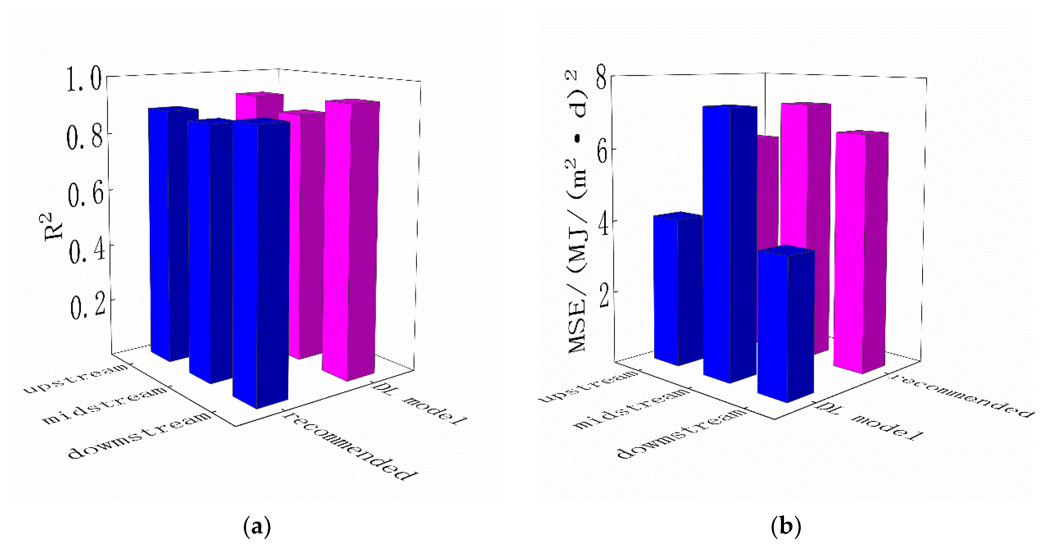
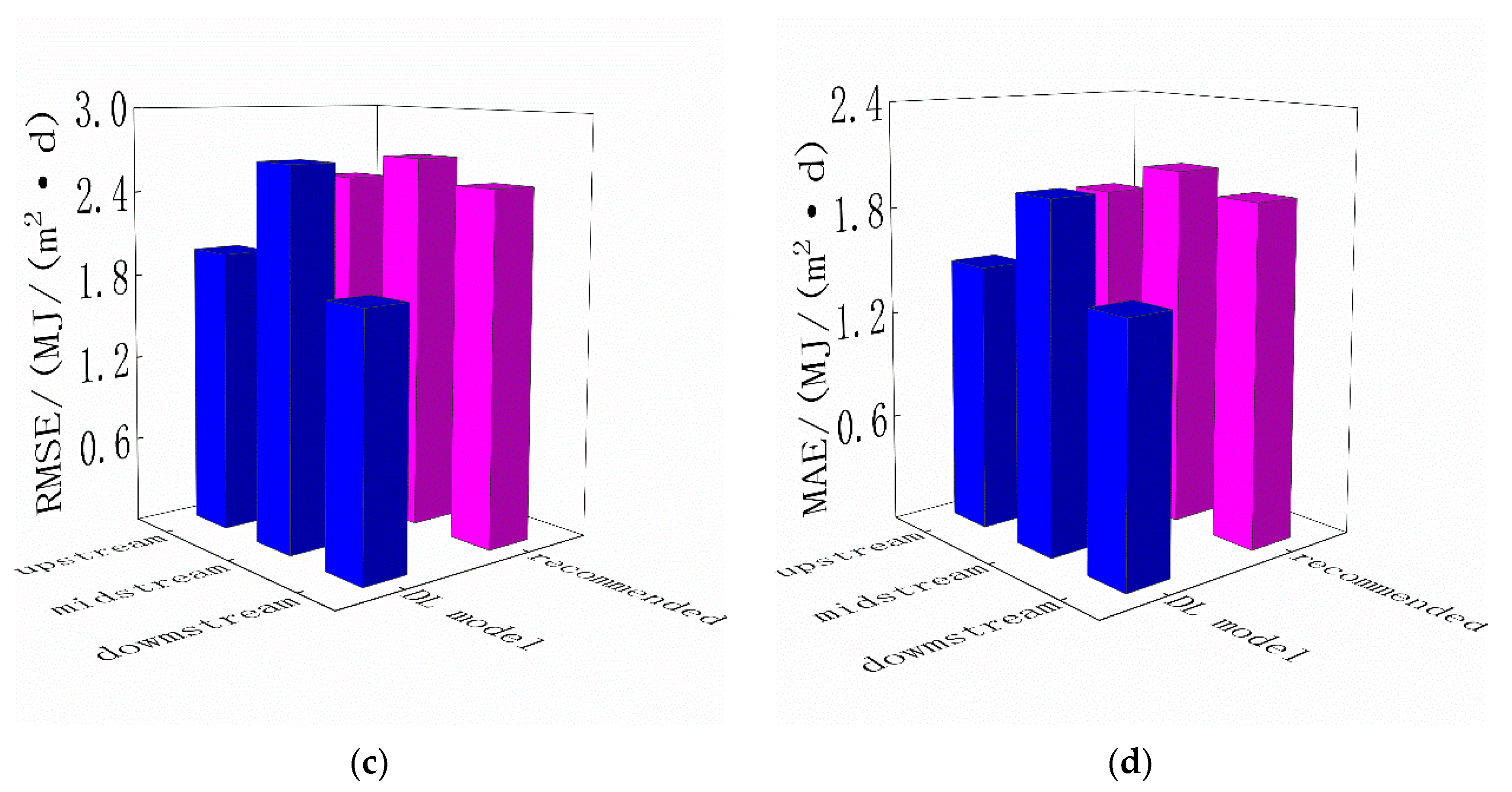
3.2. Comparison between the Recommended Values of Å-P Parameters and the Prediction Results of the DL Model

Solar radiation is comprehensively affected by temperature, wind speed, relative humidity, sunshine duration and other meteorological factors. On the basis of previous studies, this study selected maximum temperature T_max, minimum temperature T_min, average temperature T_avg, wind speed U, relative humidity RH, sunshine duration H and maximum sunshine duration H_max as input values to establish the DL model. The prediction results of each station in the Yellow River Basin by the Å-P parameter values recommended by FAO were compared with those of the DL model, and R^2, MSE, RMSE and MAE were used for evaluation. The comparison results are shown in

Table 3. Performance comparison between the prediction results of the recommended values of station Å-P parameters and the prediction results of the DL model.

Site	Model	R2	MSE	RMSE	MAE	Site	Model	R2	MSE	RMSE	MAE
Yushu	Recommended	0.77	9.347	3.057	2.335	Wulatezhongqi	Recommended	0.92	5.090	2.256	1.590
	DL prediction	0.90	5.018	2.240	1.728		DL prediction	0.95	3.273	1.809	1.435
Guoluo	Recommended	0.87	7.383	2.717	2.111	Dongsheng	Recommended	0.92	4.324	2.079	1.456
	DL prediction	0.88	7.343	2.710	2.207		DL prediction	0.91	6.990	2.644	1.685
Gangcha	Recommended	0.91	4.698	2.167	1.735	Taiyuan	Recommended	0.87	6.333	2.516	1.878
	DL prediction	0.94	2.647	1.627	1.243		DL prediction	0.89	9.559	3.092	2.216
Geermu	Recommended	0.93	5.999	2.449	1.984	Datong	Recommended	0.90	5.086	2.255	1.708
	DL prediction	0.96	2.033	1.426	1.029		DL prediction	0.93	3.686	1.920	1.485
Xining	Recommended	0.88	5.605	2.368	1.728	Houma	Recommended	0.89	5.979	2.445	1.835
	DL prediction	0.93	4.017	2.004	1.519		DL prediction	0.89	6.495	2.549	2.070
Ganzi	Recommended	0.89	6.954	2.637	2.172	Yanan	Recommended	0.87	8.986	2.998	2.235
	DL prediction	0.85	4.559	2.135	1.704		DL prediction	0.87	7.068	2.659	1.855
Hongyuan	Recommended	0.83	10.373	3.221	2.559	Jinghe	Recommended	0.84	8.333	2.887	2.283
	DL prediction	0.88	6.340	2.518	1.836		DL prediction	0.89	9.502	3.083	2.518
Wuwei	Recommended	0.84	9.619	3.101	2.311	Ankang	Recommended	0.84	10.803	3.287	2.489
	DL prediction	0.91	5.849	2.418	1.757		DL prediction	0.81	9.493	3.081	1.880
Minqin	Recommended	0.90	4.983	2.232	1.597	Nanyang	Recommended	0.87	5.009	2.238	1.729
	DL prediction	0.96	2.165	1.471	1.036		DL prediction	0.85	4.979	2.231	1.592
Yuzhong	Recommended	0.91	3.708	2.418	1.403	Zhengzhou	Recommended	0.88	5.487	2.342	1.736
	DL prediction	0.95	2.224	1.491	1.131		DL prediction	0.95	2.148	1.466	1.136
Guyuan	Recommended	0.91	4.270	2.066	1.486	Anyang	Recommended	0.87	9.739	3.121	2.481
	DL prediction	0.93	3.430	1.852	1.368		DL prediction	0.89	9.722	3.118	2.644
Yinchuan	Recommended	0.91	4.232	2.057	1.407	Fushan	Recommended	0.94	4.574	2.139	1.640
	DL prediction	0.94	2.629	1.621	1.163		DL prediction	0.96	1.973	1.405	1.043
Huhehaote	Recommended	0.90	5.497	2.345	1.733	Jinan	Recommended	0.86	9.697	3.114	2.368
	DL prediction	0.90	3.645	1.909	1.346		DL prediction	0.92	3.064	1.750	1.320
Erlianhaote	Recommended	0.91	6.024	2.454	1.866	Juxian	Recommended	0.92	3.105	1.762	1.344
	DL prediction	0.94	3.308	1.819	1.671		DL prediction	0.95	1.636	1.279	0.957

.

It can be seen from Table 3 that the overall prediction accuracy of the DL model in the Yellow River Basin is significantly better than the recommended values of the Å-P parameters. From the results of R², except Ganzi, Dongsheng, Ankang and Nanyang stations, the R² of other stations increases to varying degrees. The average values of R² increase from 0.88 to 0.91. The R² predicted by the Yushu station increases the most, from 0.77 to 0.90, and the R² predicted by the Ganzi station is the worst, decreasing from 0.89 to 0.85. The MSE decreases by 25.93% on average. The MSE values of the DL models of the Dongsheng, Taiyuan, Houma and Jinghe stations are greater than the recommended values of the Å-P parameters, and the MSE values of other stations decrease. The best performing station is Jinan Station. The MSE decreases from 9.697 to 3.064, which is 68.40% lower than the recommended values of the Å-P parameters. The worst performing station is Dongsheng station. Its MSE increases from 4.324 to 6.990, which is −61.55% worse than the recommended values of the Å-P parameters. RMSE has the same pattern as MSE. The RMSE of Jinan station, with the best performance, decreases from 3.114 to 1.750, which is 43.79% lower than the recommended values of the Å-P parameters. The RMSE of Dongsheng station, with the worst performance, increases from 2.079 to 2.644, which is −27.14% worse than the recommended values of the Å-P parameters. The MAE is reduced by 16.04% on average compared with the Å-P equation. Except that the DL model prediction results of the Guoluo, Dongsheng, Taiyuan, Houma, Jinghe and Anyang stations are greater than the recommended values of the Å-P parameters, the MAE values of other stations are reduced. Golmud is the best performing station, and its MAE is reduced from 0.984 to 1.029, which is 48.13% better than the recommended values of the Å-P parameters. The worst performing station is Taiyuan station, whose MAE value increases from 1.878 to 2.216, which is −18.03% worse than the recommended values of the Å-P parameters.

In general, the DL model has the best prediction results in Golmud. Compared with the recommended values of the Å-P parameters, R² is improved from 0.93 to 0.96. MSE, RMSE and MAE are reduced by 66.11%, 41.79% and 48.13%, respectively. The prediction results of Dongsheng station are the worst. Compared with the recommended values of the Å-P parameters, R² decreases from 0.92 to 0.91, and the recommended values of MSE, RMSE and MAE decrease by −61.65%, −27.14% and −15.77%, respectively, compared with the Å-P equation.

Figure 2 shows the performance comparison between the predicted results of the recommended values of the Å-P parameters and the predicted results of the DL model in the upstream, midstream and downstream of the Yellow River Basin. From Figure 2a, it can be seen that, in the upstream, midstream and downstream of the Yellow River Basin, the R² predicted by the DL model is better than the recommended values of the Å-P parameters. Among the prediction results of the upstream, midstream and downstream of the Yellow River Basin, the prediction results of the downstream are the best. Its R² increases from 0.894 to 0.934, followed by the prediction results of the upstream, whose R² increases from 0.888 to 0.921. The prediction results of the midstream are the worst. Its R² increases from 0.869 to 0.874. From Figure 2b, it can be seen that the MSE of the DL model in the upstream and downstream of the Yellow River Basin is significantly better than the recommended values of the Å-P parameters, and there is little difference between the MSE in the midstream of the Yellow River Basin and the recommended values of the Å-P parameters. Among them, the MSE in the downstream of the Yellow River Basin decreases the most, from 6.520 to 3.709, and in the upstream of the Yellow River Basin, the MSE decreases from 6.13 to 4.092. From Figure 2c, it can be seen that RMSE and MSE have the same trend in the upstream, midstream and downstream of the Yellow River Basin. RMSE decreases the most in the downstream of the Yellow River Basin, from 2.496 to 1.804, followed by the upstream of the Yellow River Basin, from 2.477 to 1.981. The worst is in the midstream of the Yellow River Basin, from 2.661 to 2.659. From Figure 2d, it can be seen that MAE decreases in different degrees in the upstream, midstream and downstream of the Yellow River Basin. Similar to the changes of other indicators, MAE decreases the most in the downstream of the Yellow River Basin, from 1.914 to 1.420. It decreases from 1.842 to 1.491 in the upstream of the Yellow River Basin and from 2.022 to 1.945 in the midstream of the Yellow River Basin.

In general, the evaluation metrics of the DL model are significantly better than the recommended values of the Å-P parameters in the upstream, midstream and downstream of the Yellow River Basin. Among them, the overall prediction results of the downstream are the best. R² increases from 0.894 to 0.934. MSE, RMSE and MAE are reduced by 43.12%, 27.73% and 25.80% respectively, followed by the overall prediction effect of the upstream: R² increases from 0.888 to 0.921; MSE, RMSE and MAE are reduced by 33.27%, 20.02% and 19.04%, respectively. The overall prediction results of the midstream are the worst. The prediction accuracy of the DL model is not different from the recommended values of the Å-P parameters. R² increases from 0.869 to 0.874, and MSE, RMSE and MAE are reduced by −0.50%, 0.07% and 3.82%, respectively.

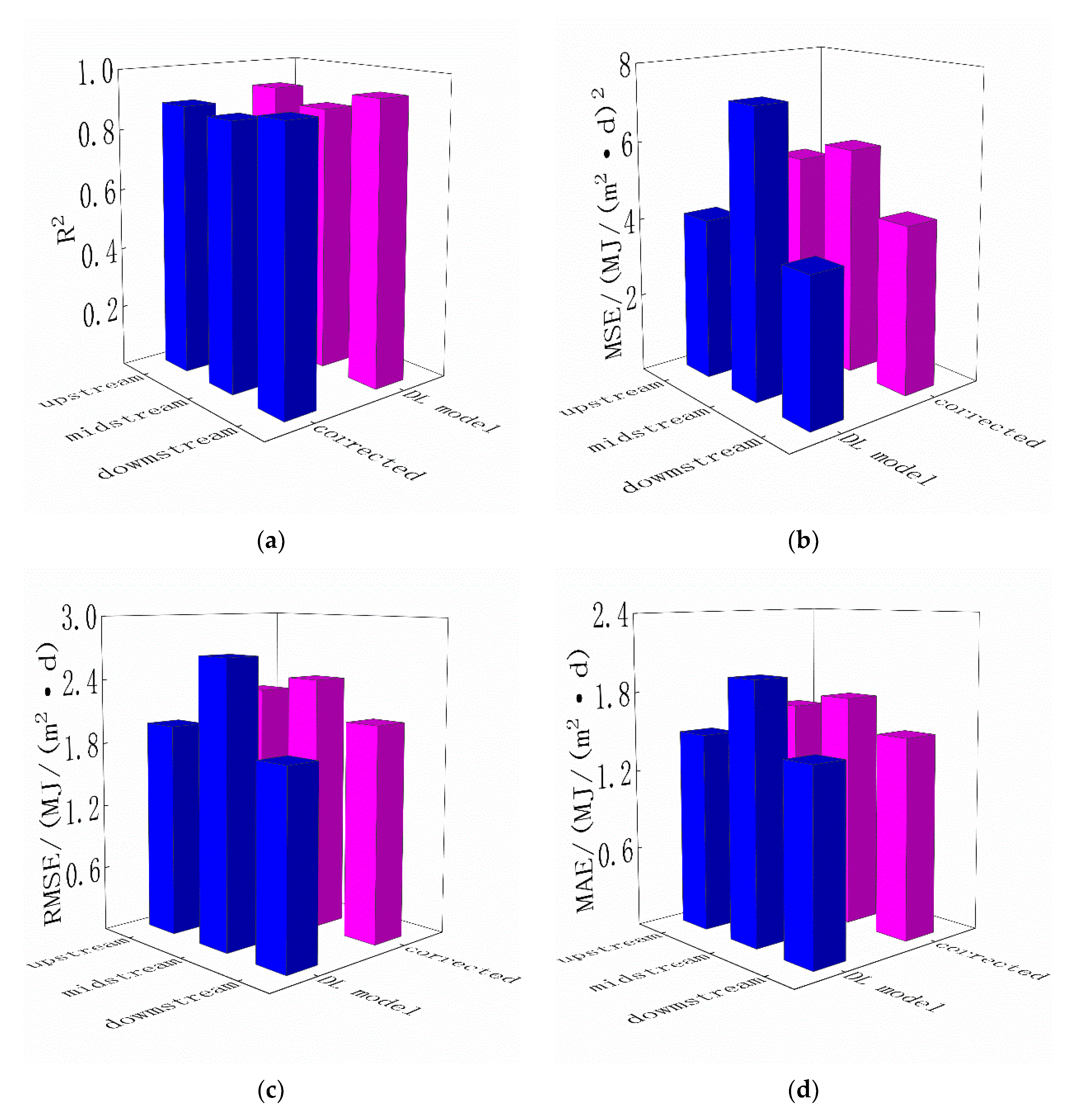
3.3. Comparison between the Prediction Results of Corrected Values of Å-P Parameters and Those of the DL Model

The Å-P parameter values recommended are proposed by FAO based on the average regional climate of foreign countries for many years; the prediction accuracy in China is poor. We will compare the prediction results of the Å-P parameter values corrected based on the measured data of stations in the Yellow River Basin with those of the DL model. R², MSE, RMSE and MAE were also used to evaluate the prediction results of the two indexes, and the evaluation results are shown in

Table 4. Performance comparison between the prediction results of the corrected values of the Å-P parameters and the prediction results of the DL model.

Site	Model	R2	MSE	RMSE	MAE	Site	Model	R2	MSE	RMSE	MAE
Yushu	Corrected	0.78	8.926	2.988	2.209	Wulatezhongqi	Corrected	0.92	4.556	2.135	1.448
	DLprediction	0.90	5.018	2.240	1.728		DLprediction	0.95	3.273	1.809	1.435
Guoluo	Corrected	0.87	5.085	2.255	1.608	Dongsheng	Corrected	0.92	3.831	1.957	1.391
	DLprediction	0.88	7.343	2.710	2.207		DLprediction	0.91	6.990	2.644	1.685
Gangcha	Corrected	0.92	3.285	1.812	1.314	Taiyuan	Corrected	0.88	5.476	2.340	1.750
	DLprediction	0.94	2.647	1.627	1.243		DLprediction	0.89	9.559	3.092	2.216
Geermu	Corrected	0.94	3.226	1.796	1.290	Datong	Corrected	0.90	4.989	2.234	1.698
	DLprediction	0.96	2.033	1.426	1.029		DLprediction	0.93	3.686	1.920	1.485
Xining	Corrected	0.88	5.449	2.334	1.687	Houma	Corrected	0.89	5.040	2.245	1.654
	DLprediction	0.93	4.017	2.004	1.519		DLprediction	0.89	6.495	2.549	2.070
Ganzi	Corrected	0.89	3.467	1.862	1.408	Yanan	Corrected	0.88	5.871	2.423	1.718
	DLprediction	0.85	4.559	2.135	1.704		DLprediction	0.86	7.068	2.659	1.855
Hongyuan	Corrected	0.84	7.648	2.765	1.994	Jinghe	Corrected	0.83	7.641	2.764	2.007
	DLprediction	0.88	6.340	2.518	1.836		DLprediction	0.89	9.502	3.083	2.518
Wuwei	Corrected	0.81	12.101	2.960	2.760	Ankang	Corrected	0.83	7.185	2.680	1.871
	DLprediction	0.91	5.849	2.418	1.757		DLprediction	0.81	9.493	3.081	1.880
Minqin	Corrected	0.90	4.684	2.164	1.614	Nanyang	Corrected	0.88	4.448	2.109	1.506
	DLprediction	0.96	2.165	1.471	1.036		DLprediction	0.85	4.979	2.231	1.592
Yuzhong	Corrected	0.91	3.661	2.418	1.485	Zhengzhou	Corrected	0.89	4.685	2.165	1.615
	DLprediction	0.95	2.224	1.491	1.131		DLprediction	0.95	2.148	1.466	1.136
Guyuan	Corrected	0.92	3.859	1.964	1.427	Anyang	Corrected	0.88	4.657	2.158	1.597
	DLprediction	0.93	3.430	1.852	1.368		DLprediction	0.89	9.722	3.118	2.644
Yinchuan	Corrected	0.92	4.201	2.050	1.381	Fushan	Corrected	0.94	2.528	1.590	1.205
	DLprediction	0.94	2.629	1.621	1.163		DLprediction	0.96	1.973	1.405	1.043
Huhehaote	Corrected	0.90	4.967	2.229	1.595	Jinan	Corrected	0.86	6.647	2.578	1.835
	DLprediction	0.90	3.645	1.909	1.346		DLprediction	0.92	3.064	1.750	1.320
Erlianhaote	Corrected	0.91	5.108	2.260	1.584	Juxian	Corrected	0.93	2.848	1.688	1.266
	DLprediction	0.94	3.308	1.819	1.671		DLprediction	0.95	1.636	1.279	0.957

.

It can be seen from Table 4 that the prediction accuracy of the DL model is significantly better than the corrected values of the Å-P parameters at most stations in the Yellow River Basin. From the results of R², the prediction accuracy of the DL model is greatly improved compared with the corrected values of the Å-P parameters, and the average value of R² increases from 0.89 to 0.91. Among them, the R² values of the Ganzi, Dongsheng, Taiyuan, Yan’an, Ankang and Nanyang stations decrease, and the prediction results of the DL model of Ankang station are the worst. Compared with the corrected values of the Å-P parameters, R² decreases from 0.83 to 0.81. Compared with the corrected values of the Å-P parameters, the R² values of other stations increase to varying degrees. The prediction results of the Golmud, Minqin and Fushan stations are the best, with R² reaching 0.96. Compared with the Å-P parameters, the corrected values of the Yushu station increase the most, and R² increases from 0.78 to 0.90. The MSE decreases by 5.93% on average. Except for Datong, the MSE values of the DL model in the midstream of the Yellow River Basin are higher than the corrected values of the Å-P parameters. In addition, the MSE values of the Guoluo, Ganzi and Anyang stations are also greater than the corrected values of the Å-P parameters. The MSE value of the DL model in Anyang station is the largest, 9.722, which is −108.75% lower than the corrected values of the Å-P parameters. The MSE values of other stations are lower than the corrected values of the Å-P parameters. The MSE value of Zhengzhou station is reduced from 4.685 to 2.148, a decrease of 54.15%. The values of RMSE have the same trend as MSE, with an average decrease of 5.56%. Anyang station is the worst station, and the value of RMSE increases from 2.158 to 3.118, a decrease of −44.48% compared with the Å-P equation. The best station is Zhengzhou station. The value of RMSE is reduced to 1.466 from 2.165, which is 32.29% lower than that of the Å-P equation. The average decrease of MAE is 2.28%, and the pattern of MAE is similar to that of MSE and RMSE. Anyang station has the worst performance, and its MAE value has increased from 1.597 to 2.644, an increase of 65.59%. Wuwei station has the best performance, and its MAE value has decreased from 2.760 to 1.757, a decrease of 36.34% compared with the corrected values of the Å-P parameters.

In general, the DL model has the best prediction results in Zhengzhou station. Compared with the corrected values of the Å-P parameters, R² is improved from 0.89 to 0.95, and MSE, RMSE and MAE are reduced by 54.15%, 32.29% and 29.64%, respectively. The prediction results of Anyang station are the worst. R² is improved from 0.88 to 0.99 compared with the corrected values of the Å-P parameters, but the prediction error is large and the corrected values of MSE, RMSE and MAE are decreased by −108.75%, −44.48% and −65.59% compared with the Å-P parameters, respectively.

Figure 3 shows the performance comparison between the predicted results of the corrected values of the Å-P parameters in the upstream, midstream and downstream of the Yellow River Basin and the predicted results of the DL model. From Figure 3a, it can be seen that, in the upstream, midstream and downstream of the Yellow River Basin, the R² predicted by the DL model is better than the corrected values of the Å-P parameters. Among the prediction results of the upstream, midstream and downstream of the Yellow River Basin, the prediction results of the downstream are the best. Its R² increases from 0.900 to 0.934, followed by the prediction results of the upstream, whose R² increases from 0.889 to 0.921. The prediction results of the midstream are the worst. Its R² increases from 0.870 to 0.874. From Figure 3b, it can be seen that the MSE values of the DL model in the upstream and downstream of the Yellow River Basin are significantly better than the corrected values of the Å-P parameters, and the MSE values in the midstream of the Yellow River Basin are significantly worse than the corrected values of the Å-P parameters. The MSE value decreases the most in the upstream of the Yellow River Basin, from 5.253 to 4.092. In the downstream of the Yellow River Basin, the MSE decreases from 4.273 to 3.709, and in the midstream of the Yellow River Basin, the MSE value increases from 5.807 to 7.255. It can be seen from Figure 3c that RMSE and MSE have the same trend in the upstream, midstream and downstream of the Yellow River Basin. The value of RMSE decreases the most in the upstream of the Yellow River Basin, from 2.247 to 1.981, followed by the downstream of the Yellow River Basin, from 2.036 to 1.804. In the midstream of the Yellow River Basin, the value of RMSE increases from 2.399 to 2.659. From Figure 3d, it can be seen that MAE has the same trend as MSE and RMSE in the upstream, midstream and downstream of the Yellow River Basin. It decreases the most in the upstream of the Yellow River Basin, from 1.637 to 1.491. It decreases from 1.503 to 1.420 in the downstream of the Yellow River Basin and from 1.744 to 1.945 in the midstream of the Yellow River Basin.

In general, the evaluation metrics of the DL model are significantly better than the corrected values of the Å-P parameters in the upstream and downstream of the Yellow River Basin. Among them, the overall prediction results of the upstream are the best. R² increases from 0.889 to 0.921. MSE, RMSE and MAE are reduced by 22.11%, 11.84% and 8.94%, respectively, followed by the overall prediction effect of the downstream, whose R² increases from 0.900 to 0.934 and whose MSE, RMSE and MAE are reduced by 13.21%, 11.40% and 5.55%, respectively. Compared with the corrected values of the Å-P parameters, the overall prediction results in the midstream of the Yellow River Basin are poor. R² increases from 0.870 to 0.874, but MSE, RMSE and MAE are reduced by −24.93%, −10.83% and −11.56%, respectively.

4. Discussion

4.1. Calibration of Å-P Parameters

Using an empirical model to estimate solar radiation is relatively simple, and it is easy to obtain input data with. At present, the most commonly used empirical model is the Å-P equation based on sunshine [24]. However, the application of this model is often limited by parameter correction. How to select the appropriate Å-P parameters is the focus of using this model [25].

Due to little research on the correction of the a and b parameters of the Å-P equation in various regions of China and the lack of necessary research on and understanding of how the selection of these parameters affects the estimation of solar radiation and other related variables in the past, it is still quite common to directly use the recommended values of FAO-56 in China, especially in the calculation of reference crop evapotranspiration ET₀. The a and b parameter values recommended by FAO-56 are proposed by FAO based on the multi-year average regional climate abroad. Due to the influence of clouds, geographical location, altitude and climate in different regions of China, the prediction accuracy of the FAO-56 recommended values are affected to varying degrees. In addition, Liu et al. [26] point out that correction is the best method to obtain accurate Å-P parameters. Therefore, how to reasonably correct the values of the a and b parameters according to different regions of China is the key to accurately estimating solar radiation using the Å-P equation. Based on the measured solar radiation data of 28 stations in the Yellow River Basin for many years, the parameters of the Å-P equation of each station are fitted by the least square method, and the corrected values of the Å-P parameters of each station are obtained. The calibration values of the Å-P parameters are evaluated by five evaluation metrics, namely, the determination coefficient R², rooted mean square error RMSE, relative error RE, mean absolute error MAE and consistency index d.

The Å-P parameter correction and evaluation metrics of each station in the Yellow River Basin are shown in Table 2. The value of a varies from 0.11 to 0.29, with an average of 0.18, and the value of b varies from 0.50 to 0.69, with an average of 0.58. After comparing with the corrected values of the parameters a and b obtained by Chen et al. [27] and Liu et al. [25,26] in the Yellow River basin, it can be found that the corrected values of each station are the same, with only minor differences, which may be caused by the different lengths of data records used by each station. The data record we use is much longer than that used by Chen et al. and Liu et al. The values of R² range from 0.74 to 0.96. Except for Yushu station in Qinghai Province, the R² of all other stations is above 0.80, and the average R² is 0.89. Compared with previous research results [9,25,26,27,28], our results show that our data have better quality control.

In addition, it can be seen from the evaluation metrics in Table 2 that the correction effect of the Å-P equation at the upstream and downstream stations of the Yellow River Basin is good, with R² reaching 0.90, and the correction effect at the stations in the midstream is poor, with R² at only 0.87. In general, the correction effect of the Å-P equation at the stations in the upstream of the Yellow River Basin is the best. RMSE, RE, MAE and d are 2.271, 0.14, 1.670 and 0.97, respectively, The correction effect of stations in the downstream is second, with RMSE, RE, MAE and d of 2.292, 0.18, 1.732 and 0.97, respectively. The correction effect of stations in the midstream of the Yellow River Basin is the worst, with RMSE, RE, MAE and d of 2.859, 0.22, 2.142 and 0.96, respectively. However, there is no particularly satisfactory explanation for why the correction effect of the Å-P equation is better in the upstream and downstream of the Yellow River Basin and worse in the midstream of the Yellow River Basin. A possible reason is that the parameters of the Å-P equation have a great impact on solar radiation in high altitude and high radiation areas and in low altitude and low radiation areas [19].

4.2. Comparison between DL Model and Å-P Model

The lack of measured solar radiation data has also led to the development of other indirect methods, including the method based on random weather model [29], the satellite remote sensing method [30], the linear interpolation method [31], the empirical relationship method using other meteorological variables [32] and the physical transmission method [33,34]. In recent years, with the rapid development of artificial intelligence and neural networks, the prediction of solar radiation by artificial neural networks has become more and more mature. Many researchers [11,12,13,14] estimate solar radiation by establishing an artificial neural network model and prove the feasibility of predicting solar radiation by artificial neural networks but do not compare the artificial neural network with other methods regarding prediction performance, so the superiority of artificial neural networks is not shown in predicting solar radiation. Some studies [2,35] compare the artificial neural network model with the most widely used Å-P equation and the empirical regression model proposed by other researchers [36], but the results are different. The research results of Tymvios et al. show that the prediction accuracy of artificial neural networks is similar to that of the Å-P equation, while Jiang et al. compare the artificial divine power network model with the empirical regression model proposed by other researchers [36]. It is confirmed that the artificial neural network is more suitable for the prediction of solar radiation.

In this study, the neural networks with three hidden layers (40 60 40) take the highest temperature T_max, the lowest temperature T_min, the average temperature T_avg, the wind speed U, the relative humidity RH, the sunshine hours H and the maximum sunshine hours H_max as input variables. We compare the solar radiation predicted by the DL model with the solar radiation predicted by the FAO-56 recommended values and the solar radiation predicted by the corrected values fitted by the measured data of stations in the Yellow River Basin and evaluate by four evaluation metrics: the determination coefficient R², mean square error MSE, rooted mean square error RMSE and mean absolute error MAE. The Å-P equation has higher prediction accuracy and a wider application range.

The performance comparison of the recommended values of the Å-P parameters at each station, the recommended values of the Å-P parameters at the upstream, midstream and downstream of the Yellow River Basin and the prediction results of the DL model are shown in Table 3 and Figure 2, respectively. From Table 3 and Figure 2, it can be seen that the overall prediction accuracy of the DL model in the Yellow River Basin is significantly better than the recommended values of the Å-P parameters. R² increases from 0.88 to 0.91, and MSE, RMSE and MAE are reduced by 25.93% 16.25% and 16.04% on average, respectively, which is consistent with the conclusion of Jiang et al. However, the difference is that, according to the analysis of the results of each station, the predicted solar radiation of the DL model is not better than the recommended values of the Å-P parameters at all stations. For example, the solar radiation predicted by the DL model at the Dongsheng, Taiyuan, Houma and Jinghe stations is poor, among which Dongsheng station has the worst prediction result, and its R² (0.92) is worse than the recommended values of the Å-P parameters (0.91). MSE, RMSE and MAE decrease by −61.65%, −27.14% and −15.77%, respectively. From the above results, it can be seen that the stations with poor prediction results of the DL model are distributed in the midstream of the Yellow River Basin.

Table 4 and Figure 3 show the performance comparison between the predicted results of the Å-P parameter corrected values of each station, the corrected values of the Å-P parameters in the upstream, midstream and downstream of the Yellow River Basin and the predicted results of the DL model, respectively. From Table 4 and Figure 3, it can be seen that the overall prediction accuracy of the DL model in the Yellow River Basin is slightly better than the corrected values of the Å-P parameters. R² increases from 0.89 to 0.91, and MSE, RMSE and MAE are reduced by 5.93%, 5.56% and 2.28%, respectively. The results show that using the DL model to predict solar radiation in the Yellow River Basin is an effective alternative method. From the results of the upstream, midstream and downstream of the Yellow River basin, compared with the recommended and corrected values of the Å-P parameters, the DL model has the same pattern, that is, the prediction results are better in the upstream and downstream of the Yellow River Basin but worse in the midstream of the Yellow River Basin. This result is also consistent with the trend of the correction results of the Å-P equation. Therefore, we speculate that the prediction results of the DL model in the midstream of the Yellow River basin may be related to the low accuracy of the input variables.

4.3. Comparison between DL Model and Other Machine Learning Models

With the rise of machine learning algorithms, building a solar radiation prediction model by machine learning algorithms has become a hot research direction at present. A large number of researchers have applied different machine learning algorithms into solar radiation prediction models and have achieved good prediction results. Chen et al. [15] used the meteorological data of three stations in Liaoning Province to establish seven support vector machine models with different inputs. The average RMSE values of the three stations are 2.325 MJ/m², 1.915 MJ/m² and 2.040 MJ/m². Zeng et al. [37] used random forest (RF) to build a model for predicting China’s daily solar radiation. The overall correlation coefficient R of the model is 0.95, and the root mean square error RMSE value is 2.34 MJ/m². Huang et al. [38] predicted and compared the daily and monthly solar radiation values of Ganzhou City by building 12 machine learning models. The R² values of the 12 machine learning models predicting the daily solar radiation values were between 0.838–0.925, and the RMSE values of the 12 machine learning models were between 1.987–2.999 MJ/m². The best machine learning model was the GBRT (gradient enhanced regression tree) model, with R² values of 0.925 and RMSE values of 1.987 MJ/m². The R² value of the DL model constructed in this paper is 0.910, and the RMSE value is 2.148 MJ/m² in the Yellow River Basin. Among them, the prediction accuracy in the lower reaches of the Yellow River Basin is the highest, with an R² value of 0.934 and an RMSE value of 1.804 MJ/m². Compared with the DL model constructed in this paper, it can be found that the prediction accuracy of the DL model constructed in this paper is better than that of most machine learning models.

From a solar radiation prediction point of view, the machine learning models can learn the complex nonlinear characteristics from different inputs so as to improve their prediction accuracy, but only for smaller datasets. In practice, the machine learning models cannot accurately predict relatively large datasets [39]. In addition, compared with traditional machine learning models, deep learning models such as recurrent neural networks (RNN), long-term and short-term memory neural networks (LSTM) and convolutional neural networks (CNN) have shown the potential to further improve the accuracy of solar radiation prediction. Zhu et al. [40] proposed a Siamese convolutional neural network-long short-term memory (SCNN-LSTM) model to predict the inter-hour DNI by combining the time-dependent spatial features of total sky images and historical meteorological observations, which can predict the solar radiation ten minutes in advance, and the performance is better than the published methods. Mishra et al. [41] proposed a new short-term solar radiation prediction model based on the concepts of long-term and short-term memory network (LSTM) and wavelet transform (WT), and it showed superior performance compared with other machine learning models. The above research results show that deep learning models not only have a wider application range and higher prediction accuracy but also can realize the ultra short-term solar radiation prediction with the rapid development of the deep learning architecture. Therefore, deep learning models are more suitable for predicting long-term and short-term changes of solar radiation.

5. Conclusions

Taking the measured meteorological data of the highest temperature T_max, lowest temperature T_min, average temperature T_avg, wind speed U, relative humidity RH, sunshine hours H and maximum sunshine hours H_max as input variables, this study establishes a DL model for predicting solar radiation in the Yellow River Basin of China and compares it with the recommended and corrected values of the Å-P equation parameters widely used at present. The determination coefficient R², mean square error MSE, root mean square error RMSE and mean absolute error MAE are evaluated.

Compared with the Å-P equation using the recommended values of FAO-56, the prediction accuracy of the DL model in the Yellow River Basin is significantly improved. R² is increased from 0.883 to 0.910, and MSE, RMSE and MAE are reduced by 25.30%, 15.94% and 16.22%, respectively. Among them, the prediction accuracy in the downstream of the Yellow River Basin is the best, followed by the upstream. Compared with the Å-P equation using corrected values, the R² of the DL model is increased from 0.887 to 0.910, and the MSE, RMSE and MAE are reduced by 1.82%, 3.57% and 0.57%, respectively. Among them, the prediction accuracy of the DL model in the upstream and downstream of the Yellow River Basin is much better than that of the Å-P equation using corrected values. The prediction accuracy of the DL model in the midstream of the Yellow River Basin is worse than that of the Å-P equation using corrected values.

In general, the ability of the DL model to accurately predict solar radiation in the upstream and downstream of the Yellow River Basin in China is significantly better than that of the Å-P empirical model. However, the application of the DL model in the midstream of the Yellow River Basin does not perform well in predicting solar radiation, which may be related to the low accuracy of input variables.

References

1. Adaramola, M.S. Estimating global solar radiation using common meteorological data in Akure, Nigeria. Renew. Energy 2012, 47, 38–44. [Google Scholar] [CrossRef]
2. Tymvios, F.S.; Jacovides, C.P.; Michaelides, S.C.; Scouteli, C. Comparative study of Angstroem’s and artificial neural networks’ methodologies in estimating global solar radiation. Sol. Energy 2005, 78, 752–762. [Google Scholar] [CrossRef]
3. Liu, X.; Xu, C.; Zhong, X.; Li, Y.; Yuan, X.; Cao, J. Comparison of 16 models for reference crop evapotranspiration against weighing lysimeter measurement. Agric. Water Manag. 2017, 184, 145–155. [Google Scholar] [CrossRef]
4. Vázquez, R. Effect of potential evapotranspiration estimates on effective parameters and performance of the MIKE SHE-code applied to a medium-size catchment. J. Hydrol. 2003, 270, 309–327. [Google Scholar] [CrossRef]
5. Labed, S.; Lorenzo, E. The impact of solar radiation variability and data discrepancies on the design of PV systems. Renew. Energy 2004, 29, 1007–1022. [Google Scholar] [CrossRef]
6. Ghoneim, A. Design optimization of photovoltaic powered water pumping systems. Energy Convers. Manag. 2006, 47, 1449–1463. [Google Scholar] [CrossRef]
7. Iziomon, M.; Mayer, H. Assessment of some global solar radiation parameterizations. J. Atmos. Solar-Terrestrial Phys. 2002, 64, 1631–1643. [Google Scholar] [CrossRef]
8. Trnka, M.; Žalud, Z.; Eitzinger, J.; Dubrovský, M. Global solar radiation in Central European lowlands es-timated by various empirical formulae. Agric. For. Meteorol. 2005, 131, 54–76. [Google Scholar] [CrossRef]
9. Podestá, G.P.; Núñez, L.; Villanueva, C.A.; Skansi, M.A. Estimating daily solar radiation in the Argentine Pampas. Agric. For. Meteorol. 2004, 123, 41–53. [Google Scholar] [CrossRef]
10. Liu, Y.; Tan, Q.; Pan, T. Determining the Parameters of the Ångström-Prescott Model for Estimating Solar Radiation in Different Regions of China: Calibration and Modeling. Earth Space Sci. 2019, 6, 1976–1986. [Google Scholar] [CrossRef]
11. Al-Alawi, S.M.; Al-Hinai, H.A. An ANN-based approach for predicting global radiation in locations with no direct meas-urement instrumentation. Renew. Energy 1998, 14, 199–204. [Google Scholar] [CrossRef]
12. Mohandes, M.; Rehman, S.; Halawani, T. Estimation of global solar radiation using artificial neural networks. Renew. Energy 1998, 14, 179–184. [Google Scholar] [CrossRef]
13. Reddy, K.; Ranjan, M. Solar resource estimation using artificial neural networks and comparison with other correlation models. Energy Convers. Manag. 2003, 44, 2519–2530. [Google Scholar] [CrossRef]
14. Yildiz, B.Y.; Sahin, M.; Şenkal, O.; Peştemalci, V.; Emrahoglu, N. A Comparison of Two Solar Radiation Models Using Artificial Neural Networks and Remote Sensing in Turkey. Energy Sources Part A Recover. Util. Environ. Eff. 2013, 35, 209–217. [Google Scholar] [CrossRef]
15. Chen, J.L.; Li, G.S.; Wu, S.J. Assessing the potential of support vector machine for estimating daily solar radi-ation using sunshine duration. Energy Convers. Manag. 2013, 75, 311–318. [Google Scholar]
16. Ibrahim, I.A.; Khatib, T. A novel hybrid model for hourly global solar radiation prediction using random forests technique and firefly algorithm. Energy Convers. Manag. 2017, 138, 413–425. [Google Scholar] [CrossRef]
17. Lucas, P.D.O.E.; Alves, M.A.; Silva, P.C.D.L.E.; Guimarães, F.G. Reference evapotranspiration time series forecasting with ensemble of convolutional neural networks. Comput. Electron. Agric. 2020, 177, 105700. [Google Scholar]
18. Saggi, M.K.; Jain, S. Reference evapotranspiration estimation and modeling of the Punjab Northern India using deep learning. Comput. Electron. Agric. 2018, 156, 387–398. [Google Scholar] [CrossRef]
19. Liu, X.Y.; Li, Y.Z. Effect of various Ångström–Prescott coefficients on reference crop evapotranspiration—A casestudy for the midstream of the Yellow River. Chin. Agro-Meteorol. 2007, 1, 29–35. [Google Scholar]
20. Ngström, A. Solar and ter restrial radiation. Report to the international commission for solar research on actinometric in-vestigations of sola and atmospheric radiation. Q. J. R. Meteorol. Soc. 1924, 50, 121–125. [Google Scholar] [CrossRef]
21. Prescott, J.A. Evaporation from a water surface in relation to solar radiation. Trans. R. Soc. S. Aust. 1940, 64, 114–125. [Google Scholar]
22. Rumelhart, D.E.; McClelland, J.L. (Eds.) Parallel Distributed Processing: Explorations in Themicrostructure of Cognition; MIT Press: Cambridge, MA, USA, 1986. [Google Scholar]
23. Hinton, G.E. Learning multiple layers of representation. Trends Cogn. Sci. 2007, 11, 428–434. [Google Scholar] [CrossRef]
24. Bakirci, K. Correlations for estimation of daily global solar radiation with hours of bright sunshine in Turkey. Energy 2009, 34, 485–501. [Google Scholar] [CrossRef]
25. Liu, X.; Xu, Y.; Zhong, X.; Zhang, W.; Porter, J.R.; Liu, W. Assessing models for parameters of the Ångström–Prescott formula in China. Appl. Energy 2012, 96, 327–338. [Google Scholar] [CrossRef]
26. Liu, X.; Mei, X.; Li, Y.; Zhang, Y.; Wang, Q.; Jensen, J.R.; Porter, J.R. Calibration of the Ångström–Prescott coefficients (a, b) under different time scales and their impacts in estimating global solar radiation in the Yellow River basin. Agric. For. Meteorol. 2009, 149, 697–710. [Google Scholar] [CrossRef]
27. Chen, R.; Ersi, K.; Yang, J.; Lu, S.; Zhao, W. Validation of five global radiation models with measured daily data in China. Energy Convers. Manag. 2004, 45, 1759–1769. [Google Scholar] [CrossRef]
28. Persaud, N.; Lesolle, D.; Ouattara, M. Coefficients of the Angström–Prescott equation for estimating global irradiance from hours of bright sunshine in Botswana and Niger. Agric. For. Meteorol. 1997, 88, 27–35. [Google Scholar] [CrossRef]
29. Richardson, C.W.; Wright, D.A. WGEN: A Model for Generating Daily Weather Variables; U.S. Department of Agriculture, Agricultural Research Service: Washington, DC, USA, 1984.
30. Pinker, R.; Frouin, R.; Li, Z. A review of satellite methods to derive surface shortwave irradiance. Remote Sens. Environ. 1995, 51, 108–124. [Google Scholar] [CrossRef]
31. Hay, J.E.; Suckling, P.W. An assessment of the net-works for measuring and modeling solar radiation in British Columbia and adjacent areas of western Canada. Can. Geogr. 1979, 23, 222–238. [Google Scholar] [CrossRef]
32. Bristow, K.L.; Campbell, G.S. On the relationship between incoming solar radiation and daily maximum and minimum temperature. Agric. For. Meteorol. 1984, 31, 159–166. [Google Scholar] [CrossRef]
33. Gueymard, C.A. Parameterized transmittance model for direct beam and circumsolar spectral irradiance. Sol. Energy 2001, 71, 325–346. [Google Scholar] [CrossRef]
34. de La Casinière, A.; Bokoye, A.I.; Cabot, T. Direct Solar Spectral Irradiance Measurements and Updated Simple Transmittance Models. Am. Meteorol. Soc. 1997, 36, 509–520. [Google Scholar] [CrossRef]
35. Jiang, Y. Computation of monthly mean daily global solar radiation in China using artificial neural networks and comparison with other empirical models. Energy 2009, 34, 1276–1283. [Google Scholar] [CrossRef]
36. Jin, Z.; Yezheng, W.; Gang, Y. General formula for estimation of monthly average daily global solar radiation in China. Energy Convers. Manag. 2005, 46, 257–268. [Google Scholar] [CrossRef]
37. Zeng, Z.; Wang, Z.; Gui, K.; Yan, X.; Gao, M.; Luo, M.; Geng, H.; Liao, T.; Li, X.; An, J.; et al. Daily global solar radiation in China estimated from high-density me-teorological observations: A random forest model framework. Earth Space Sci. 2020, 7, e2019EA001058. [Google Scholar] [CrossRef] [Green Version]
38. Huang, L.; Kang, J.; Wan, M.; Fang, L.; Zhang, C.; Zeng, Z. Solar Radiation Prediction Using Different Machine Learning Algorithms and Implications for Extreme Climate Events. Front. Earth Sci. 2021, 9, 202. [Google Scholar] [CrossRef]
39. Ghimire, S.; Deo, R.C.; Casillas-Pérez, D.; Salcedo-Sanz, S. Boosting solar radiation predictions with global climate models, observational predictors and hybrid deep-machine learning algorithms. Appl. Energy 2022, 316, 119063. [Google Scholar] [CrossRef]
40. Zhu, T.; Guo, Y.; Li, Z.; Wang, C. Solar Radiation Prediction Based on Convolution Neural Network and Long Short-Term Memory. Energies 2021, 14, 8498. [Google Scholar] [CrossRef]
41. Mishra, M.; Dash, P.B.; Nayak, J.; Naik, B.; Swain, S.K. Deep learning and wavelet transform integrated approach for short-term solar PV power prediction. Measurement 2020, 166, 108250. [Google Scholar] [CrossRef]
Figure 1. Framework diagram of deep learning model.
Agronomy 12 01081 g001
Figure 2. (a) The determination coefficient R2 values of the prediction results of the recommended Å-P parameters and the DL model in the upstream, midstream and downstream of the Yellow River Basin; (b) The mean square error MSE values of the prediction results of the recommended Å-P parameters and the DL model in the upstream, midstream and downstream of the Yellow River Basin; (c) The rooted mean square error RMSE values of the prediction results of the recommended Å-P parameters and the DL model in the upstream, midstream and downstream of the Yellow River Basin; (d) The mean absolute error MAE values of the prediction results of the recommended Å-P parameters and the DL model in the upstream, midstream and downstream of the Yellow River Basin.
Agronomy 12 01081 g002aAgronomy 12 01081 g002b
Figure 3. (a) The determination coefficient R2 values of the prediction results of the corrected Å-P parameters and the DL model in the upstream, midstream and downstream of the Yellow River Basin; (b) The mean square error MSE values of the prediction results of the corrected Å-P parameters and the DL model in the upstream, midstream and downstream of the Yellow River Basin; (c) The rooted mean square error RMSE values of the prediction results of the corrected Å-P parameters and the DL model in the upstream, midstream and downstream of the Yellow River Basin; (d) The mean absolute error MAE values of the prediction results of the corrected Å-P parameters and the DL model in the upstream, midstream and downstream of the Yellow River Basin.
Agronomy 12 01081 g003