
Modeling and Control of a Wheeled Biped Robot


Abstract
:1. Introduction
2. Overview of WBR
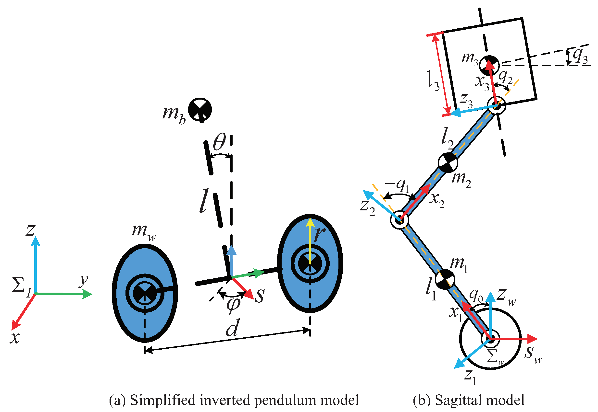
3. Dynamic Modeling
3.1. Equivalent Centroid Calculation
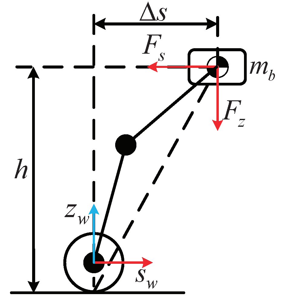
3.2. VL-WIP Modeling
3.3. Modeling of the Multi-Rigid Body System
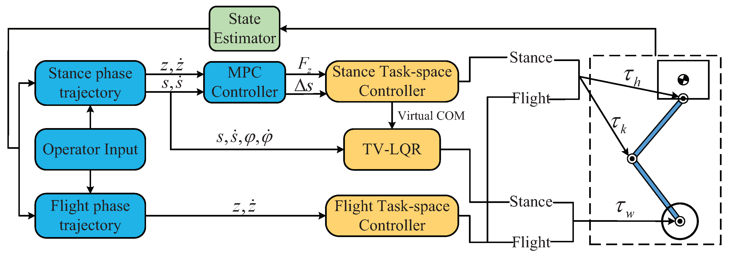
4. Control Strategy
4.1. VL-WIP Controller
4.2. Upper-Body Controller
4.3. State Estimation
5. Simulation and Experiment
5.1. Simulations
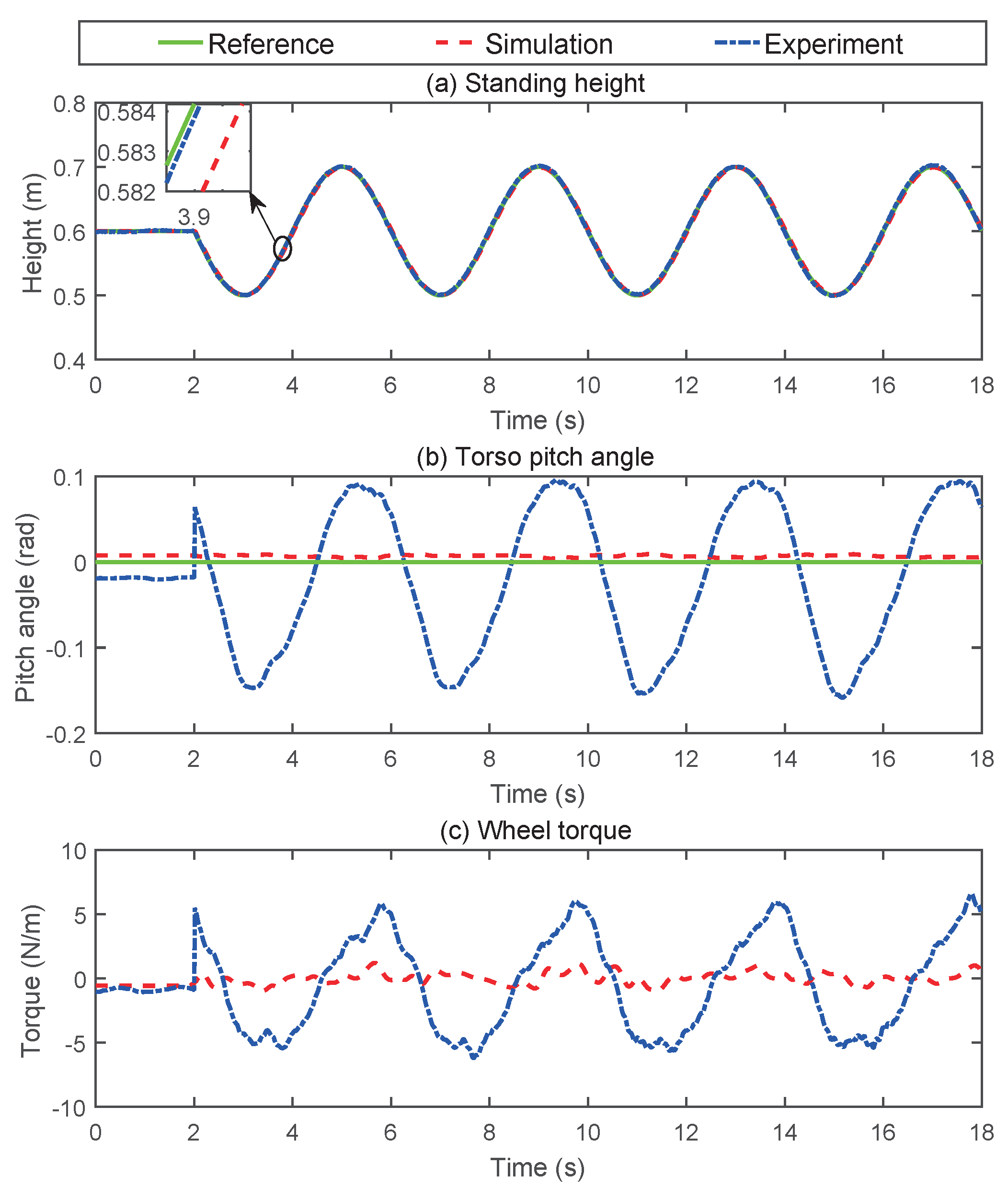
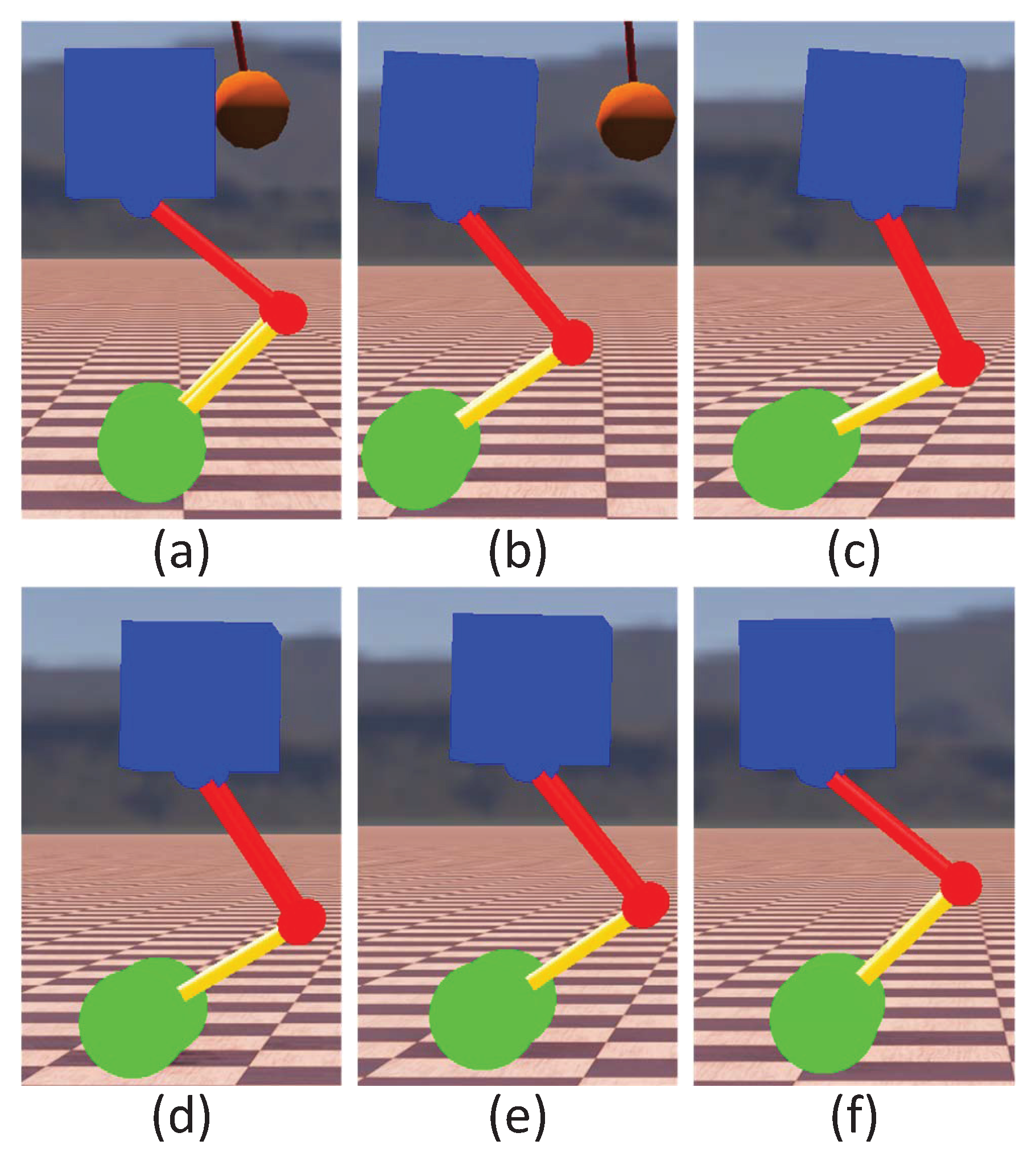
5.1.1. Changing Height
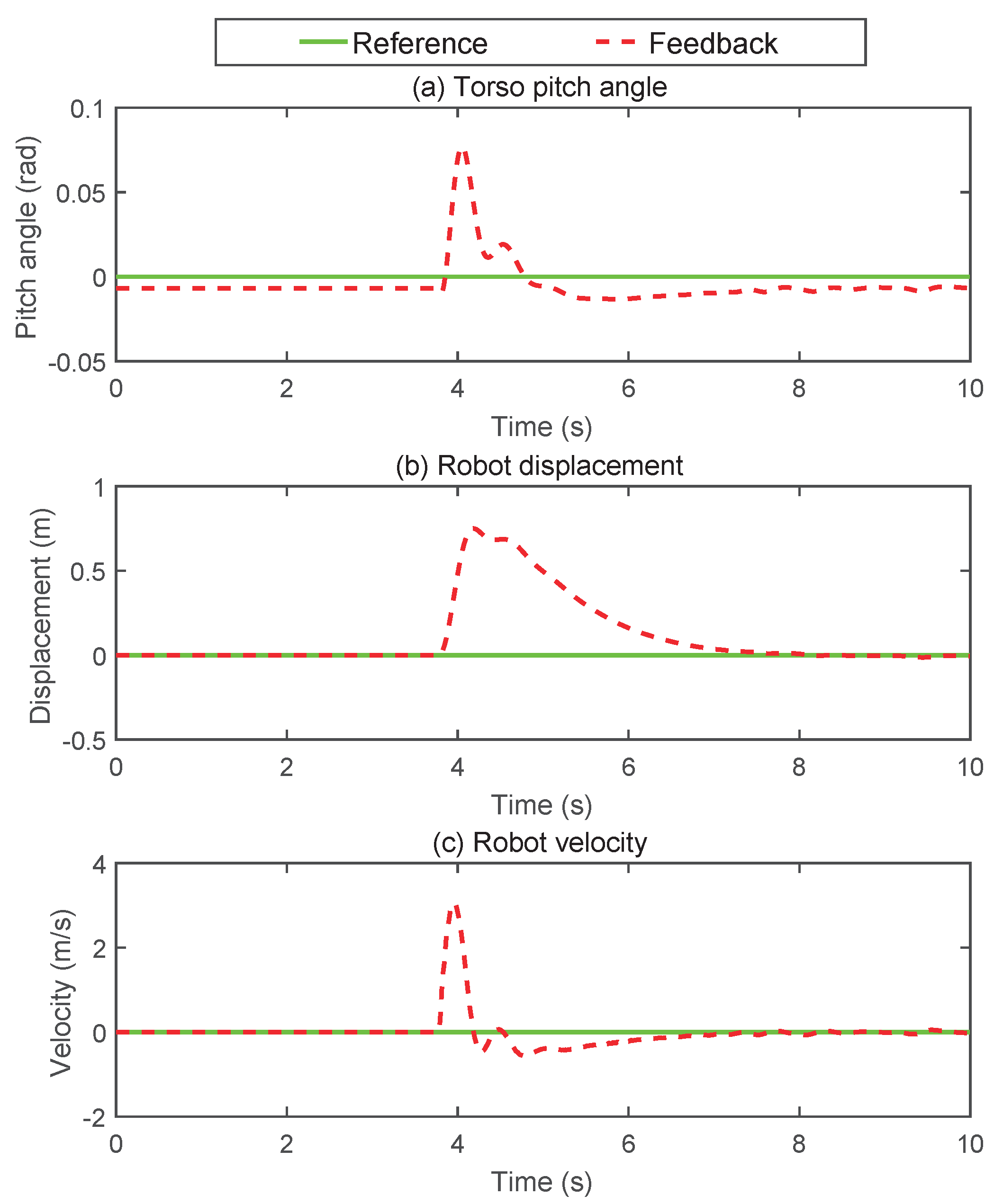
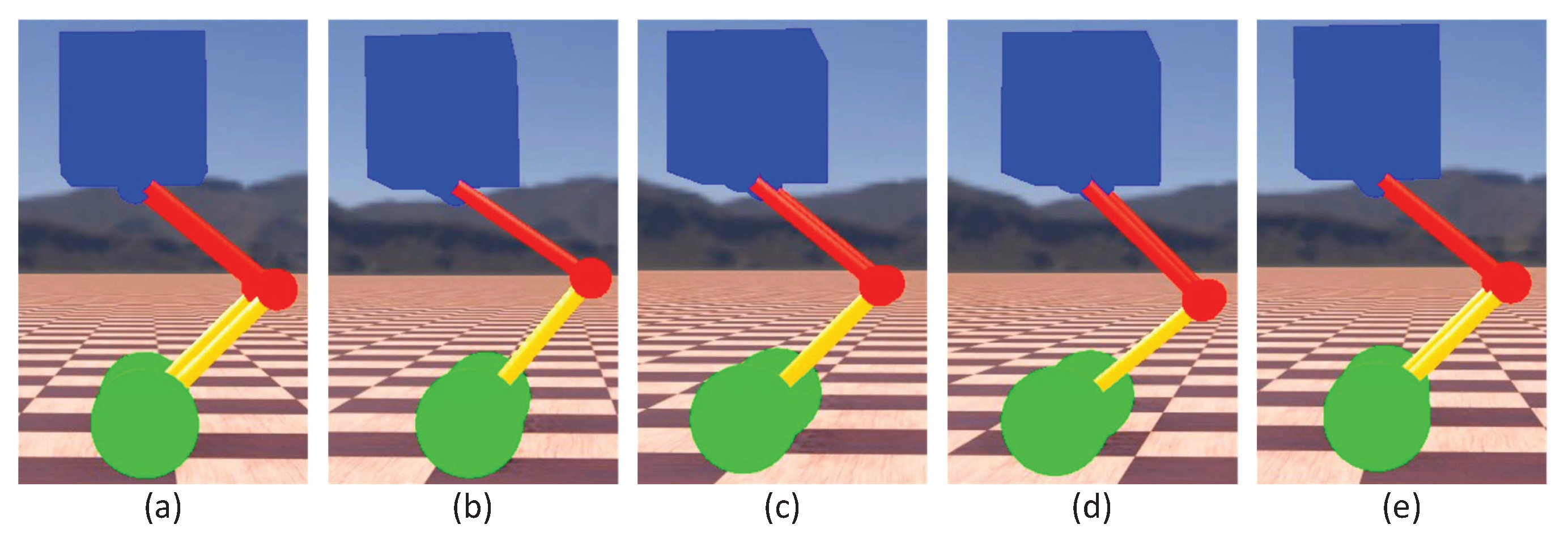
5.1.2. Sagittal Impact Recovery
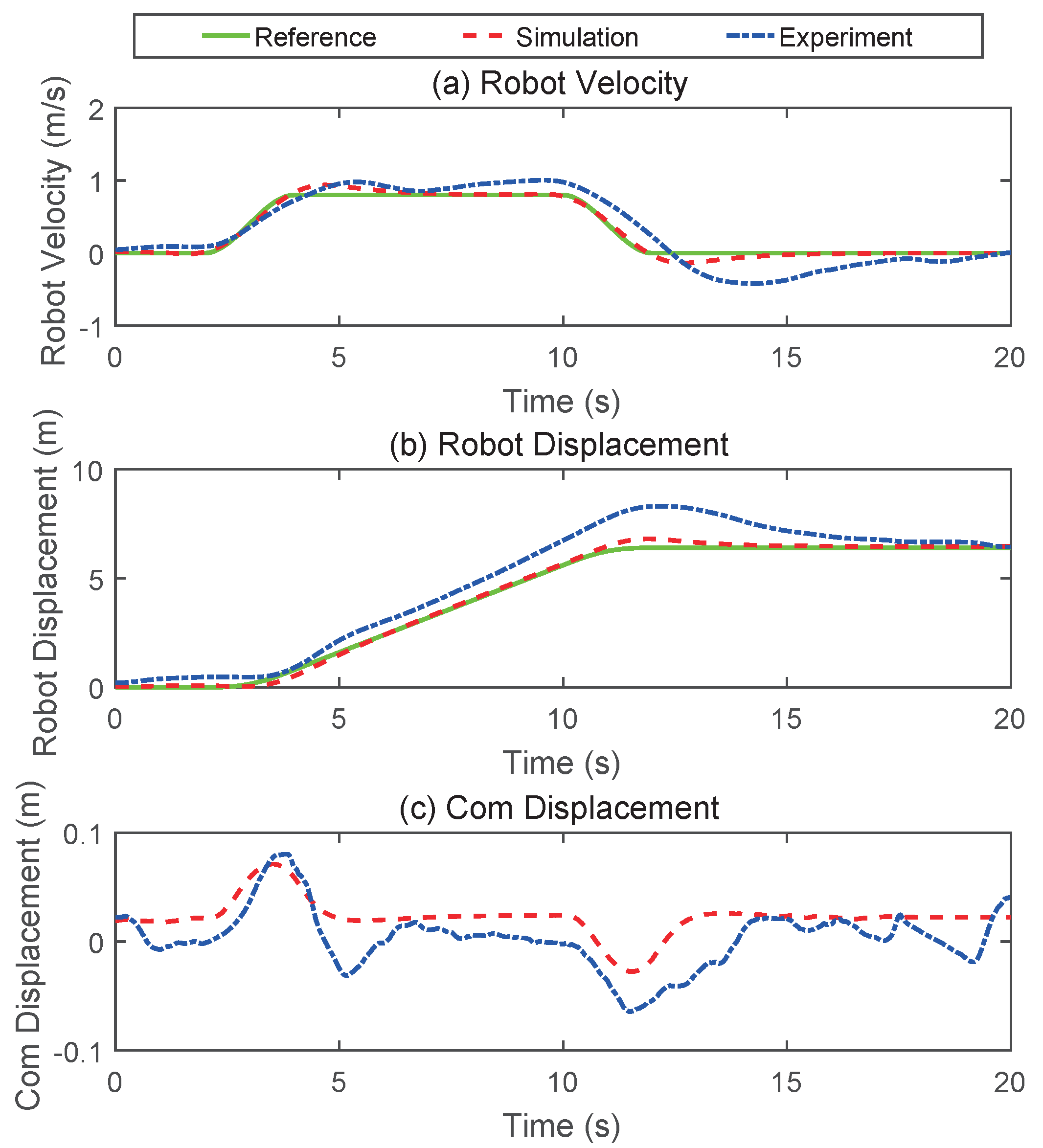
5.1.3. Velocity Tracking
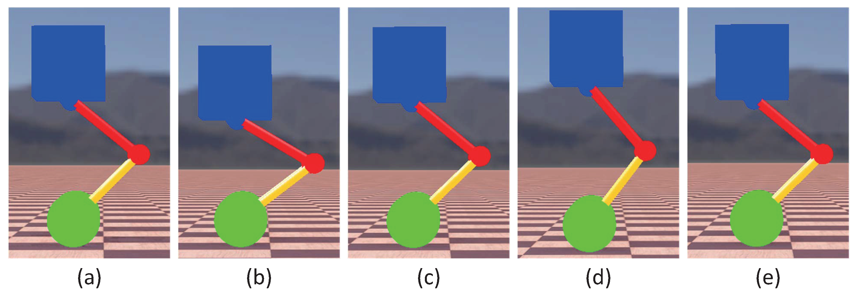
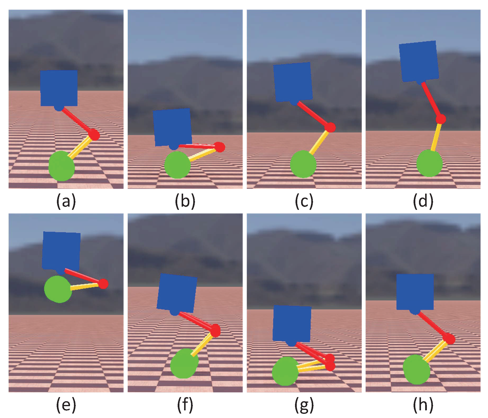
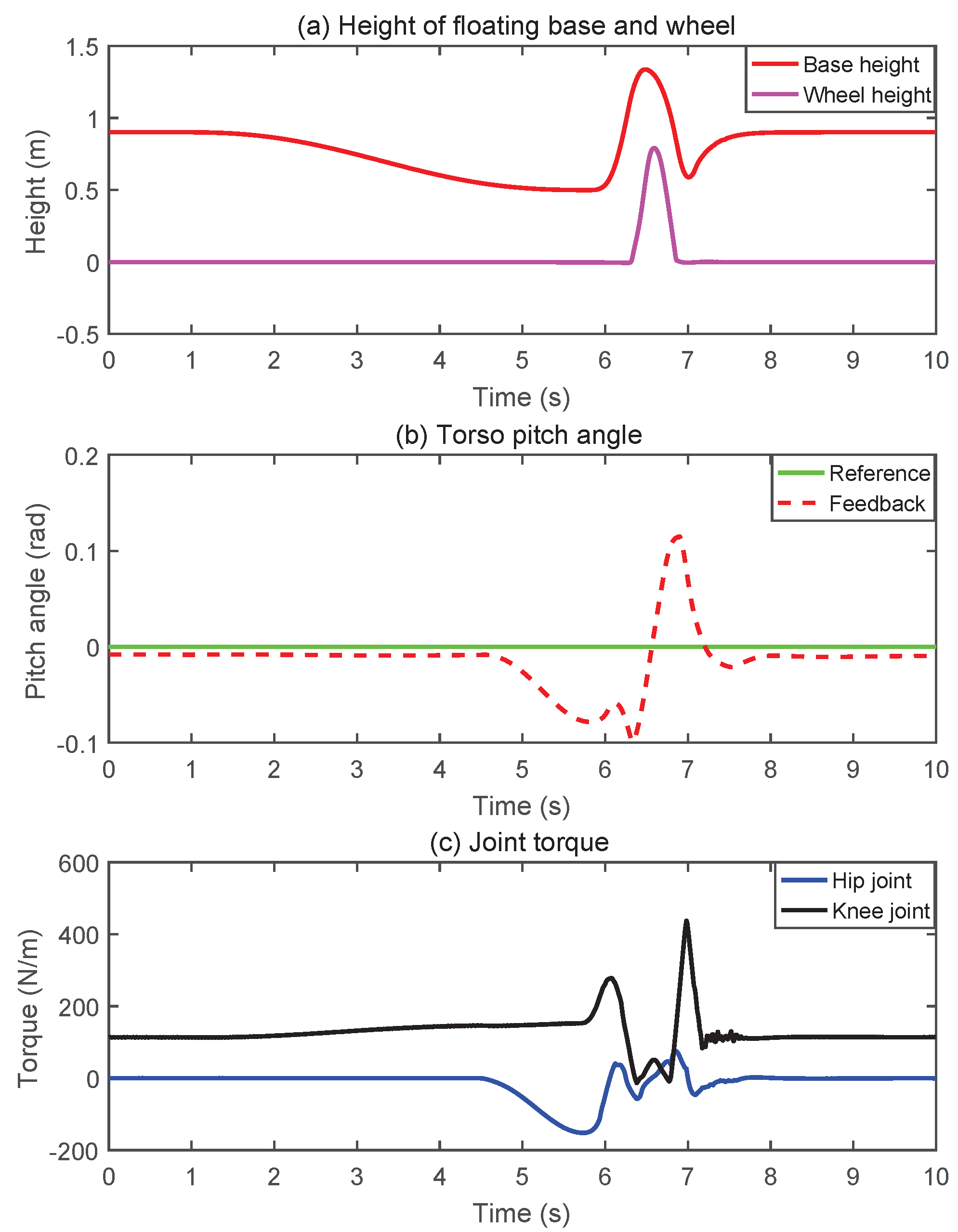
5.1.4. Jumping
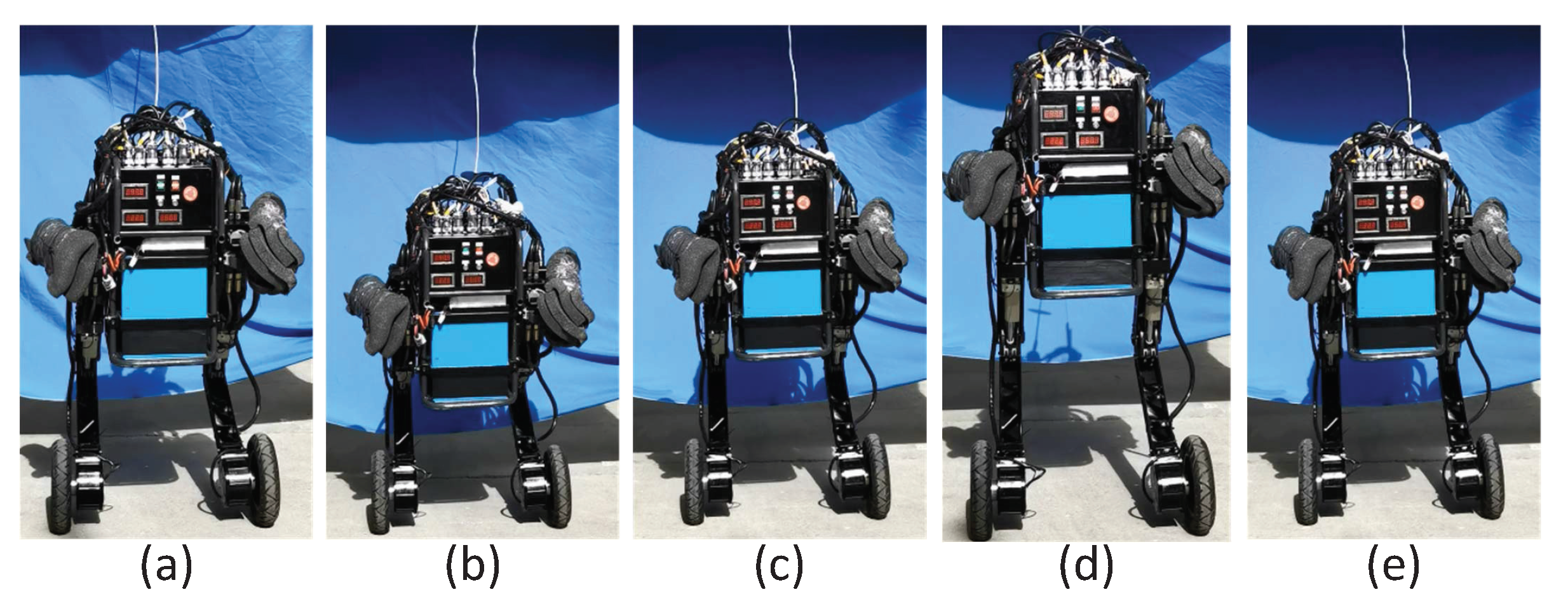
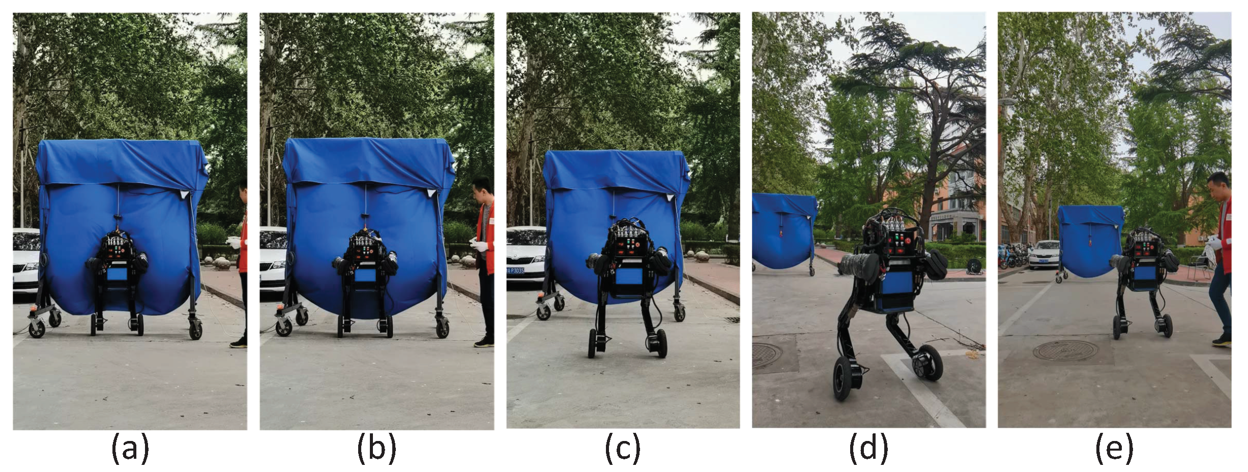
5.2. Physical Prototype Experiments
6. Conclusions and Future Work
Supplementary Materials
Author Contributions
Funding
Conflicts of Interest
References
- Xu, K.; Wang, S.; Wang, X.; Wang, J.; Chen, Z.; Liu, D. High-flexibility locomotion and whole-torso control for a wheel-legged robot on challenging terrain. In Proceedings of the 2020 IEEE International Conference on Robotics and Automation (ICRA), Paris, France, 31 May–31 August 2020; pp. 10372–10377. [Google Scholar]
- Chen, Z.; Li, J.; Wang, S.; Wang, J.; Ma, L. Flexible gait transition for six wheel-legged robot with unstructured terrains. Robot. Auton. Syst. 2022, 103989. [Google Scholar] [CrossRef]
- Bjelonic, M.; Bellicoso, C.D.; de Viragh, Y.; Sako, D.; Tresoldi, F.D.; Jenelten, F.; Hutter, M. Keep rollin’—Whole-body motion control and planning for wheeled quadrupedal robots. IEEE Robot. Autom. Lett. 2019, 4, 2116–2123. [Google Scholar] [CrossRef] [Green Version]
- Available online: https://www.youtube.com/watch?v=-7xvqQeoA8c (accessed on 28 February 2017).
- Li, X.; Zhou, H.; Feng, H.; Zhang, S.; Fu, Y. Design and experiments of a novel hydraulic wheel-legged robot (WLR). In Proceedings of the 2018 IEEE/RSJ International Conference on Intelligent Robots and Systems (IROS), Madrid, Spain, 1–5 October 2018; pp. 3292–3297. [Google Scholar]
- Li, X.; Zhou, H.; Zhang, S.; Feng, H.; Fu, Y. WLR-II, a hose-less hydraulic wheel-legged robot. In Proceedings of the 2019 IEEE/RSJ International Conference on Intelligent Robots and Systems (IROS), Macau, China, 3–8 November 2019; pp. 4339–4346. [Google Scholar]
- Klemm, V.; Morra, A.; Salzmann, C.; Tschopp, F.; Bodie, K.; Gulich, L.; Küng, N.; Mannhart, D.; Pfister, C.; Vierneisel, M.; et al. Ascento: A two-wheeled jumping robot. In Proceedings of the 2019 IEEE International Conference on Robotics and Automation (ICRA), Montreal, QC, Canada, 20–24 May 2019; pp. 7515–7521. [Google Scholar]
- Zhang, C.; Liu, T.; Song, S.; Meng, M.Q.H. System design and balance control of a bipedal leg-wheeled robot. In Proceedings of the 2019 IEEE International Conference on Robotics and Biomimetics (ROBIO), Dali, China, 6–8 December 2019; pp. 1869–1874. [Google Scholar]
- Liu, T.; Zhang, C.; Wang, J.; Song, S.; Meng, M.Q.H. Towards Terrain Adaptability: In Situ Transformation of Wheel-biped Robots. IEEE Robot. Autom. Lett. 2022, 2, 3819–3826. [Google Scholar] [CrossRef]
- Zhao, L.; Yu, Z.; Chen, X.; Huang, G.; Wang, W.; Han, L.; Qiu, X.; Zhang, X.; Huang, Q. System Design and Balance Control of a Novel Electrically-driven Wheel-legged Humanoid Robot. In Proceedings of the 2021 IEEE International Conference on Unmanned Systems (ICUS), Beijing, China, 15–17 October 2021; pp. 742–747. [Google Scholar]
- Raza, F.; Hayashibe, M. Towards robust wheel-legged biped robot system: Combining feedforward and feedback control. In Proceedings of the 2021 IEEE/SICE International Symposium on System Integration (SII), Iwaki, Japan, 11–14 January 2021; pp. 606–612. [Google Scholar]
- Xin, Y.; Rong, X.; Li, Y.; Li, B.; Chai, H. Movements and balance control of a wheel-leg robot based on uncertainty and disturbance estimation method. IEEE Access. 2019, 7, 133265–133273. [Google Scholar] [CrossRef]
- Wang, S.; Cui, L.; Zhang, J.; Lai, J.; Zhang, D.; Chen, K.; Zheng, Y.; Zhang, Z.; Jiang, Z. Balance control of a novel wheel-legged robot: Design and experiments. In Proceedings of the 2021 IEEE International Conference on Robotics and Automation (ICRA), Xi’an, China, 30 May–5 June 2021; pp. 6782–6788. [Google Scholar]
- Klemm, V.; Morra, A.; Gulich, L.; Mannhart, D.; Rohr, D.; Kamel, M.; Viragh, Y.; Siegwart, R. LQR-assisted whole-body control of a wheeled bipedal robot with kinematic loops. IEEE Robot. Autom. Lett. 2020, 5, 3745–3752. [Google Scholar] [CrossRef]
- Xin, Y.; Chai, H.; Li, Y.; Rong, X.; Li, B.; Li, Y. Speed and acceleration control for a two wheel-leg robot based on distributed dynamic model and whole-body control. IEEE Access. 2019, 7, 180630–180639. [Google Scholar] [CrossRef]
- Zhou, H.; Li, X.; Feng, H.; Li, J.; Zhang, S.; Fu, Y. Model decoupling and control of the wheeled humanoid robot moving in sagittal plane. In Proceedings of the 2019 IEEE-RAS 19th International Conference on Humanoid Robots (Humanoids), Toronto, ON, Canada, 15–17 October 2019; pp. 1–6. [Google Scholar]
- Chen, H.; Wang, B.; Hong, Z.; Shen, C.; Wensing, P.M.; Zhang, W. Underactuated motion planning and control for jumping with wheeled-bipedal robots. IEEE Robot. Autom. Lett. 2020, 6, 747–754. [Google Scholar] [CrossRef]
- Bledt, G. Regularized Predictive Control Framework for Robust Dynamic Legged Locomotion. Ph.D. Thesis, Massachusetts Institute of Technology, Cambridge, MA, USA, 2020. [Google Scholar]
- Kim, D.; Di Carlo, J.; Katz, B.; Bledt, G.; Kim, S. Highly dynamic quadruped locomotion via whole-body impulse control and model predictive control. arXiv 2019, arXiv:1909.06586. [Google Scholar]
- Gibson, G.; Dosunmu-Ogunbi, O.; Gong, Y.; Grizzle, J. Terrain-Aware Foot Placement for Bipedal Locomotion Combining Model Predictive Control, Virtual Constraints, and the ALIP. arXiv 2021, arXiv:2109.14862. [Google Scholar]
- Ding, Y.; Pandala, A.; Li, C.; Shin, Y.H.; Park, H.W. Representation-free model predictive control for dynamic motions in quadrupeds. IEEE Trans. Robot. 2021, 37, 1154–1171. [Google Scholar] [CrossRef]
- Di Carlo, J.; Wensing, P.M.; Katz, B.; Bledt, G.; Kim, S. Dynamic locomotion in the mit cheetah 3 through convex model-predictive control. In Proceedings of the 2018 IEEE/RSJ International Conference on Intelligent Robots and Systems (IROS), Madrid, Spain, 1–5 October 2018; pp. 1–9. [Google Scholar]
- Kajita, S.; Kanehiro, F.; Kaneko, K.; Fujiwara, K.; Harada, K.; Yokoi, K.; Hirukawa, H. Biped walking pattern generation by using preview control of zero-moment point. In Proceedings of the 2003 IEEE International Conference on Robotics and Automation (ICRA), Taipei, Taiwan, 14–19 September 2003; pp. 1620–1626. [Google Scholar]
- Wieber, P.B. Trajectory free linear model predictive control for stable walking in the presence of strong perturbations. In Proceedings of the 2006 6th IEEE-RAS International Conference on Humanoid Robots (Humanoids), Genova, Italy, 4–6 December 2006; pp. 137–142. [Google Scholar]
- Wensing, P.M.; Wang, A.; Seok, S.; Otten, D.; Lang, J.; Kim, S. Proprioceptive actuator design in the mit cheetah: Impact mitigation and high-bandwidth physical interaction for dynamic legged robots. IEEE Trans. Robot. 2017, 33, 509–522. [Google Scholar] [CrossRef]
- Zhou, Y.; Wang, Z.; Chung, K.W. Turning motion control design of a two-wheeled inverted pendulum using curvature tracking and optimal control theory. J. Optim. Theory Appl. 2019, 181, 634–652. [Google Scholar] [CrossRef] [Green Version]
- Goswami, A.; Kallem, V. Rate of change of angular momentum and balance maintenance of biped robots. In Proceedings of the 2004 IEEE International Conference on Robotics and Automation (ICRA), New Orleans, LA, USA, 26 April–1 May 2004; pp. 3785–3790. [Google Scholar]
- Jerez, J.L.; Kerrigan, E.C.; Constantinides, G.A. A condensed and sparse QP formulation for predictive control. In Proceedings of the 2011 50th IEEE Conference on Decision and Control and European Control Conference, Orlando, FL, USA, 12–15 December 2011; pp. 5217–5222. [Google Scholar]
- Pratt, J.; Chew, C.M.; Torres, A.; Dilworth, P.; Pratt, G. Virtual model control: An intuitive approach for bipedal locomotion. Int. J. Robot. Res. 2001, 20, 129–143. [Google Scholar] [CrossRef]
- Bloesch, M.; Hutter, M.; Hoepflinger, M.A.; Leutenegger, S.; Gehring, C.; Remy, C.D.; Siegwart, R. State estimation for legged robots-consistent fusion of leg kinematics and IMU. Robotics 2013, 17, 17–24. [Google Scholar]
- Kalman, R.E. A new approach to linear filtering and prediction problems. Trans. ASME–J. Basic Eng. 1960, 82, 35–45. [Google Scholar] [CrossRef] [Green Version]


| Parameter | Description | Value |
|---|---|---|
| Mass of the wheel | 3.5 kg | |
| Moment of inertia of the wheel | 0.1 kg · m | |
| l | Length of the pendulum | / |
| Tilt angle of the pendulum | / | |
| Yaw angle of the VL-WIP | / | |
| r | Radius of the wheel | 0.127 m |
| d | Distance between two wheels | 0.63 m |
| s | Displacement of the VL-WIP | / |
| Torque about the left wheel | / | |
| Torque about the right wheel | / | |
| Mass of the upper body | 73 kg | |
| Moment of inertia about the y-axis | ||
| Moment of inertia about the z-axis | 3.3 kg · m | |
| Mass of the shank | 1.2 kg | |
| Mass of the thigh | 5.3 kg | |
| Mass of the torso | 60 kg | |
| Length of the shank | 0.45 m | |
| Length of the thigh | 0.45 m | |
| Height of the torso | 0.35 m | |
| Angle of the ankle joint | ||
| Angle of the knee joint | / | |
| Angle of the hip joint | / | |
| Pitch angle of the torso | / |
Publisher’s Note: MDPI stays neutral with regard to jurisdictional claims in published maps and institutional affiliations. |
© 2022 by the authors. Licensee MDPI, Basel, Switzerland. This article is an open access article distributed under the terms and conditions of the Creative Commons Attribution (CC BY) license (https://creativecommons.org/licenses/by/4.0/).
Share and Cite
Cui, Z.; Xin, Y.; Liu, S.; Rong, X.; Li, Y. Modeling and Control of a Wheeled Biped Robot. Micromachines 2022, 13, 747. https://doi.org/10.3390/mi13050747
Cui Z, Xin Y, Liu S, Rong X, Li Y. Modeling and Control of a Wheeled Biped Robot. Micromachines. 2022; 13(5):747. https://doi.org/10.3390/mi13050747
Chicago/Turabian StyleCui, Zemin, Yaxian Xin, Shuyun Liu, Xuewen Rong, and Yibin Li. 2022. "Modeling and Control of a Wheeled Biped Robot" Micromachines 13, no. 5: 747. https://doi.org/10.3390/mi13050747