Ocean Eddies in the Drake Passage: Decoding Their Three-Dimensional Structure and Evolution

Abstract

The Drake Passage is known for its abundant mesoscale eddies, but little is known about their three-dimensional characteristics, which hinders our understanding of their impact on eddy-induced transport and deep-sea circulation. A 10-year study was conducted using GLORYS12 Mercator Ocean reanalysis data from 2009 to 2018. The study analyzed the statistical characteristics of eddies in the Drake Passage, spanning from the surface down to a depth of 2000 m in three dimensions. The findings indicate that the mean radius of the eddies is 35.5 km, with a mean lifespan of 12.3 weeks and mean vorticity of 2.2 × 10⁻⁵ s⁻¹. The eddies are most active and energetic near the three main fronts and propagate north-eastward at an average distance of 97.8 km. The eddy parameters vary with water depth, with more anticyclones detected from the surface to 400 m, displaying a larger radius and longer propagation distance. Cyclones have longer lifespans and greater vorticity. However, beyond 400 m, there is not much difference between anticyclones and cyclones. Approximately 23.3% of the eddies reach a depth of 2000 m, with larger eddies tending to penetrate deeper. The eddies come in three different shapes, bowl-shaped (52.7%), lens-shaped (27.1%) and cone-shaped (20.2%). They exhibit annual and monthly distribution patterns. Due to its high latitude location, the Drake Passage has strong rotation and weak stratification, resulting in the generation of small and deep-reaching eddies. These eddies contribute to the formation of Antarctic intermediate water and lead to modulation of turbulent dissipation.

1. Introduction

The Drake Passage (shown in Figure 1), a narrow and deep stretch of water that separates South America and the Antarctic Peninsula, serves as a choke point for the Antarctic Circumpolar Current (ACC), and plays significant role in the global oceanic and atmospheric systems [1]. The ACC flows through the Drake Passage from the south-west to the north-east, and it comprises three major fronts, namely, the Sub-Antarctic Front (SAF), the South Polar Front (PF) and the South Antarctic Circumpolar Current (SACCF), which are arranged from north to south [2]. The peculiar topographical features and instability of these fronts contribute to the formation of eddies [3,4]. Additionally, the presence of strong winds, large waves and intense currents in the area also play a crucial role in the formation and dynamics of ocean eddies in the Drake Passage.

Recent research has focused on understanding the behavior and dynamics of ocean eddies in the Drake Passage, which are important for the meridional transport of heat, salt and nutrients across the ACC and their influence on biogeochemistry. The strong zonal ACC creates a significant obstacle for cross-frontal interaction, but eddies can overcome this barrier by reducing potential vorticity gradients, flattening the isopycnals and facilitating cross-frontal transport [6,7]. Early analyses rely on ship measurements and mostly focus on individual eddies. Joyce, et al. [8] observed that the polar front was curved toward the equator to form a cold-core cyclone ring of 100 km diameter that drifted in a 5–10 cm s⁻¹ direction to the north-east. Subsequent research by Hofmann and Whitworth [3] found that mesoscale activity within the Drake Passage is dominated by the migration of three cold-core rings and one warm-core ring within the SACCF north to the SAF south. In recent years, with the increasing availability of satellite observations and improvements in numerical models, extensive research on eddies in the Drake Passage have been carried out. The eddies in the Drake Passage are mainly distributed between the three fronts, with higher eddy kinetic energy between SAF and PF [9]. The number of eddies varies monthly, with a higher number of anticyclones occurring from March to May, while a greater number of cyclones happen in July and August [10]. Eddies in the Drake Passage are mainly generated by the oblique pressure instability near the front. The meandering of fronts due to rugged bottom topography and twisting, narrow, deep canyons result in the continuous shedding of cyclones and anticyclones [11]. The anticyclonic eddies are generated in coherence with the meandering of PF and SACCF, while the cyclones are mainly from the southern fronts associated with Ona Rise and Terror Rise [12]. Additionally, the eddies in the Drake Passage lead to a northward shift of the front [13], and the eddy momentum force affects the strength and number of ACC fronts [14].

In terms of the contribution of eddies to the meridional heat and salt transport, the values of meridional heat transfer in the ACC region range from −0.4 to −1.1 PW [15]. Along the mid-ACC path, the transient eddies are almost entirely responsible for transporting heat fluxes across the front [16]. Seasonally, the poleward eddies in the Antarctic frontal zone have the strongest eddy heat fluxes in the fall and winter [6]. Furthermore, eddies have a significant impact on distribution of biota and phytoplankton [17]. They can cause phytoplankton blooms around islands, and generate interannual variability in phytoplankton [18,19]. The eddies shed by fronts in the Drake Passage can transport high chlorophyll water up to 100 km offshore [20], and contribute carbon and nutrients that maintain the iron supply and phenology of phytoplankton blooms [21]. The frontal eddies generated in the ACC make cross-frontal fish transport possible [22].

Previous research has focused on the surface characteristics of eddies, including their interactions with fronts, biogeochemical processes and energy transport in the Drake Passage. However, the lack of research into the three-dimensional structures of eddies has limited our understanding of their dynamics and effects. The three-dimensional structures of eddies are essential in their development, sustenance and dissipation [23]. In recent years, many studies have been dedicated to exploring the three-dimensional structure of eddies in several oceans. For example, the three-dimensional structures of eddies in the South China Sea (SCS) have been constructed and discussed using a combination of moored and altimeter data [24]. More than 7000 Argo profiles have been used to determine the composition of the three-dimensional structure of eddies [25]. Additionally, research on the three-dimensional eddy structure in the SCS has been aided by the use of underwater gliders and AUVs [24,26]. Global 3D eddy statistics show that there is a clear latitudinal dependence of eddies, with “small and deep-reaching” eddies at high latitudes playing an important role in linking the deep ocean circulation and the surface circulation [27]. In the ACC, most of the eddies are deep (~2000 m), and have shorter, more chaotic trajectories compared to other seas, with propagation in all directions [28]. However, due to the frequent strong storms and harsh weather conditions in the Drake Passage, observations of the eddies are less frequent than in other areas. Therefore, most studies eddies in the ACC have focused on individual 3D eddy structures [29]. Studies on the 3D structure of eddies in the entire Drake Passage area are lacking, which limits our understanding of eddy induced material and energy transport and the distribution of biological process in the region. To address this, we use 10-year (2009–2018) GLORYS12 Mercator Ocean reanalysis data to identify and track the eddies in the Drake Passage and study their statistically characteristics, including position, number, radius, lifetime and penetrating depth and their 3D structures, etc. This study is the most comprehensive work on the three-dimensional structures of eddies in the Drake Passage, and can provide insights into eddy-induced transport, and help to reveal the linkage between the surface and deep-sea circulation.

The paper is structured as follows: Section 2 provides the materials and methods to detect eddies. Eddy dataset evaluation, the characteristics and three-dimensional structures of mesoscale eddies are discussed in Section 3. Finally, the discussion is provided in Section 4.

2. Materials and Methods

2.1. Materials

The GLORYS12 is a reanalysis product of global eddy-resolving physical ocean and sea ice reanalysis data at 1/12° horizontal resolution, covering the period from 1993 to 2018, produced by Mercator Ocean International in the context of the Copernicus Marine Environment Monitoring Service (CMEMS, https://marine.copernicus.eu, accessed on 13 January 2022) [30]. The system is based largely on the current real-time global forecasting CMEMS system [30,31], with ocean observations assimilated through a reduced-order Kalman filter. GLORYS12 assimilates the along-track sea level anomaly (SLA) from satellite altimetric data from CMEMS [32], AVHRR satellite sea surface temperature (SST) from NOAA, Ifremer/CERSAT sea-ice concentration [33] and in situ temperature and salinity vertical profiles from the latest CORA in situ databases [34,35]. Note that the CORA product integrated both data from autonomous platforms (Argo profiles, fixed moorings, gliders, drifters, sea mammals) and vessels (CTDs, XBTs, ferrybox). Compared to the deeper area, no CORA profiles are available in shallow area north of YB, so, in this area, GLORYS could be less accurate. Through quality assessments, GLORYS12 captures the main climate interannual variability signals for oceans [30,31]. It has 50 vertical levels, the velocity standard deviation of GLORYS12 data decreases from the surface down to a minimum of around 2000 m [36]. Ten years’ worth (2009–2018) of data above 2000 m were used to our study, with an uneven interval interpolation: the interval is 50 m for depths up to 150 m, 100 m for depths ranging from 200 to 700 m and 200 m for depths between 800 and 2000 m. GLORYS12 is a widely used and applicable dataset in the Drake Passage, exhibiting good agreement with Argo profiling floats [30]. In addition, a comparison of its EKE with that of the AVISO product shows a good agreement [31], and the general eddy structures and intensities in GLORYS12 align with altimeter data [37]. Moreover, the GLORYS12 data performed well in the Drake Passage, with a 99% agreement with measured data [36,38].

We incorporate the “Mesoscale Eddy Trajectory Atlas” product in our analysis (wombat.ceoas.oregonstate.edu, accessed on 13 January 2022). Eddies in this dataset are detected from the spatially high-pass filtered daily SLA of AVISO, which is considered the most popular eddy dataset [39] and is provided by Chelton, et al. (2011) [40]. The dataset provides global eddy characteristics, including eddy track, location, radius, amplitude, rotation speed and polarity. For more information about this eddy dataset, please refer to Chelton, et al. (2011) [40].

2.2. Methods

In this study, mesoscale eddies are primarily detected using current velocity from GLORYS12. The eddies are identified based on their strong rotational characteristics, accompanied by convergence and divergence motions, which correspond to a positive (negative) sea level anomaly (SLA) within anticyclonic (cyclonic) eddies [41]. There are several mesoscale eddy identification methods, including closed contour [40], Okubo-Weiss (OW) [42,43], winding angle (WA) [44] and the vector geometry-based eddy detection algorithm (VG) [45]. Among these, the VG method identifies the eddy boundary based on the outmost contour of stream function. This method retains the structural consistency of an eddy, and ensures the interior water is fully trapped [46]. The method results in a recognition rate improvement and a lower excess tracking rate of 1.1% as reported in [47]. The VG method is widely used to detect eddies in different seas [48,49,50,51], and also can be used for the identification of three-dimensional eddies [52,53]. Here, we use this method for the identification of two-dimensional eddies. For more detail about the VG method, please refer to Nencioli, et al. (2011) [45].

To detect 3D eddies, we first apply the VG method to 16 layers (surface to 2000 m depth) of the velocity field to obtain information on the location, polarity, radius, generation and termination time of eddies in each depth layer. Next, we determine the vertical direction of the eddy with the same polarity and generation time. If an eddy present in layer k under the condition of $\left|s\left(i_{k+1},j_{k+1},\right.\right.\left.k+1)-s(i_k,j_k,k)\right|<\frac{1}{4}\times r\left(i_k,j_k,k\right)$, then it is taken to be present in layer k + 1. Otherwise, the depth of this eddy is considered to be in layer k. Here, the notation (i, j, k) represents the location of the eddy center in the (x,y,z) coordinate system. The $s(i_{k+1},j_{k+1},k+1)$ and $s(i_k,j_k,k)$ are the position of the eddy center in layer k and layer k+1, respectively, and $r(i_k,j_k,k)$ is the radius of the eddy in layer k [54]. More details on this method can be found in Dong, et al. (2012) [52] and Lin, et al. (2015) [53]. Finally, a discrete 3D eddy dataset is obtained, which includes the polarity, generation and termination time, penetrating depth, drift distance, radius and position of the 3D eddies.

3. Results

3.1. Evaluation of GLORYS12 Dataset

Prior to utilizing GLORYS12 for eddy detection, we conducted a comparison of the surface kinetic energy (EKE) distribution between GLORYS12 and AVISO, as well as the 1/12° HYCOM data (Figure 2). The spatial distribution pattern of EKE obtained from GLORYS12 is consistent with the altimeter data, showing that a high value of EKE is located in a general north-east to south-west direction, along the path of ACC [12]. This direction corresponds with the three main fronts between the Subantarctic front and the Polar front, particularly north of the Yaghan Basin and the Northeast Scotia Sea Basin [37]. GLORYS12 exhibits higher EKE intensity compared to AVISO, due to its higher resolution (1/12°), which reveals more frontal and eddy instabilities and submesoscale processes like filaments around the three main fronts (Figure 2b). AVISO’s lower resolution (1/4°) results in a lower EKE intensity at the same location. Additionally, the flow field of AVISO only consists of geostrophic currents, which is another contributing factor (Figure 2a). In contrast, the EKE distribution of HYCOM has a weak correlation with AVISO, with the maximum EKE found in the north of the Yaghan Basin and along the south-west part of SAF, which differs from the other two datasets (Figure 2c). GLORYS12 and HYCOM display relatively consistent vertical EKE distributions at different depths in the Drake Passage. EKE generally decreases with water depth (Figure 3). As depicted in Figure 3, the surface exhibits the highest EKE values, with average values of 271.3 cm² s⁻², 492.4 cm² s⁻² and 317.8 cm² s⁻² obtained from AVISO, HYCOM and GLORYS12, respectively. The mean EKE difference between GLORYS12 and HYCOM at the surface is 174.6 cm² s⁻², but the difference between GLORYS12 and AVISO is 46.5 cm² s⁻². GLORYS12 data is different from the HYCOM model data in shallower depths, but similar to the AVISO data. Below 50 m, mean EKE from GLORYS12 and HYCOM are nearly identical. As depth increases, the mean EKE decreases to a minimum of 76.2 and 77.4 cm² s⁻² for GLORYS12 and HYCOM, respectively, at a depth of 2000 m (Figure 3).

Quality assessments were conducted on global ocean 1/12° physical reanalysis GLORYS12V1 [30,31]. The mean zonal velocity from 2003–2016 at 15 m and 900 m between GLORYS12 and the observation results (that are not assimilated in situ and Argo data) were compared. The results showed that the general circulation pattern, including major currents and their intensity, were well-represented in the Drake Passage. The vertical distribution of GLORYS12′s annual mean temperature was evaluated and compared to the Argo results. As shown in Figure 4a, the annual mean temperature varied with water depth. In the upper 250 m, the mean temperature of GLORYS12 was slightly higher than that of Argo by approximately 0.1–0.2 °C. The largest difference between the two datasets was at the bottom of the thermocline (about 110 m), reaching 0.32 °C. Beyond a depth of 250 m, the average temperature of GLORYS12 was approximately 0.12 °C lower than that of Argo. The vertical sections along 57.5°S (Figure 4b,c) showed similar patterns, with the average temperature in the west Drake Passage being higher than that in the east. In the western part of 60°W, a significant warm core temperature was observed, with the warm water mass extending to a depth of 1200 m. On the other hand, the two cold cores were located in the eastern region of the Drake Passage, with one cold core presented at the upper 200 m, and the other extending from 800 m to 2000 m. Moreover, in the upper 200 m, the warm core of GLORYS12 was more extensive than Argo, while the range was smaller at deeper depths. Correspondingly, the cold anomaly amplitude at depths of 800 m in GLORYS12 was larger, and the area was smaller than that of Argo. Overall, the vertical distribution of the annual average temperature for the two datasets was relatively consistent.

We further applied the VG method to identify eddies in AVISO, HYCOM and GLORYS12. A snapshot from each dataset is randomly selected and displayed in Figure 4. The eddies detected by GLORYS12 in the Drake Passage are more consistent with background flow field in AVISO than in HYCOM, which is similar to the EKE distribution (Figure 3). The larger and stronger eddies are primarily located near the three main fronts, while the meanders of the PF near the Northeast Scotia Sea Basin are more likely to shed eddies (Figure 5). Conversely, fewer eddies were detected in the north-west of the Drake Passage. Although HYCOM currents are stronger, fewer eddies were detected from the HYCOM data (Figure 5c). Therefore, GLORYS12 is better for eddy detection in the Drake Passage.

For statistical characteristics, the eddies detected by GLORYS12 are compared with the “Mesoscale Eddy Trajectory Atlas” product in the Drake Passage (45°W–70°W, 55°S–65°S). To reduce noise during eddy detection, several constraints are applied. Firstly, for the VG eddy detection method, at least three adjacent gird boxes are required, since the horizontal resolution of GLORYS12 is 1/12°, eddies with an average radius less than 25 km are removed, to avoid the misidentification of elongated features as eddies. Although eddies are ubiquitous in the Drake Passage, and short-lived eddies also play an important role in air-sea interactions in the area, eddies with lifetimes of less than 8 weeks are excluded in order to prevent uncertainty caused by the detection and tracking procedure, and to ensure the eddies are persistent.

There are two methods for counting the number of eddies: Lagrangian and Eulerian. The former considers the entire lifespan of an eddy as one, while the latter identifies one snapshot of an eddy as one. For example, if an eddy survived for 100 days, with Eulerian methods, it would have had 100 snapshots. Using the Lagrangian method, we tracked a total of 680 eddies over a 10-year period (2009–2018), including 332 cyclones (CEs) and 348 anticyclones (AEs) in the Drake Passage. For the Eulerian method, we detected a total of 58,540 eddy snapshots, of which 28,804 were cyclones and 29,736 were anticyclones. The number of AEs was slightly higher than CEs.

In comparison to GLORYS12 model results, the “Mesoscale Eddy Trajectory Atlas” dataset displays a total of 557 eddies, including 261 CEs and 296 AEs. The number of eddies detected by GLORYS12 was 22.1% higher than that of “Mesoscale Eddy Trajectory Atlas” dataset. The spatial distribution patterns between GLORYS12 results, and the “Mesoscale Eddy Trajectory Atlas” dataset (shown in Figure 6a,b) exhibit no significant contrast. The main concentration of the largest eddies is around three main fronts, particularly in the southern region of the Northeast Scotia Sea Basin. The Yaghan Basin, centered at 63°W, 55°S, has a higher concentration of eddies compared to other areas, mainly because of the existence of barotropic basin modes that have energy at intra-seasonal time scales [37]. Both datasets showed a rapid decrease in eddy numbers with increasing lifetime (Figure 6c,d). In the GLORYS12 reanalysis dataset, the number of eddies with lifetimes exceeding 8, 16 and 32 weeks were 161, 44 and 2, respectively. There are slightly more AEs than CEs with lifetimes of 20 weeks or less (Figure 6c). While CEs dominated among eddies with lifetimes exceeding 32 weeks. Except for the period of 21–22 weeks, the altimeter dataset indicates a greater occurrence of anticyclones than cyclones. Specifically, there are 13 more anticyclones that have a lifespan of 8 weeks compared to cyclones with the same lifespan. The lines in Figure 6c,d have different slopes. Figure 5c shows a more rapid decrease, indicating more short-lived eddies were detected in the GLORYS12 model, but with more eddies lasting 35 weeks. In contrast, Figure 6d shows a relatively flat decrease. Overall, the two types of data show a very similar trend.

To obtain the frequency of eddies in different regions of the Drake Passage during the ten-year study period (2009–2018), we first divided the entire area into several 1° × 1° grids. Next, we counted the number of days on which eddies appeared in each grid over the ten-year period. Finally, the eddy appearing days was divided by 3652 days (the number of days in 10 years) to obtain the frequency of eddies in each grid (Figure 7a,b). Eddies with a lifetime of less than 8 weeks are distributed in almost all regions of the Drake Passage and are relatively discrete, but the frequency of eddies occurring in the north-east region is higher than that in other regions (Figure 7a). For eddies with lifespans longer than 8 weeks, most of them are concentrated in areas with water depths exceeding 2000 m, especially near the three main fronts (Figure 7b). The deeper water regions—such as the Former Phoenix Plate Basin, the Yaghan Basin and the Ona Basin, the Endurance Fracture Zone and the Shackleton Fracture Zone (see Figure 1)—have a higher frequency of eddies. The spatial distribution of eddy polarity in 1° × 1° grids for different lifespan intervals is presented in Figure 7c,d. Eddy polarity, which reflects the dominance of cyclones or anticyclones in a region, is calculated using $P=(F_{AE}-F_{CE})/(F_{AE}+F_{CE})$, where $F_{AE}$ and $F_{CE}$ are the number of anticyclones and cyclones appearing in each grid point, respectively. Hence, if P > 0, it implies that there are more anticyclones than cyclones in that grid point (as the orange bins shown), and vice versa [45,49]. The polarity of eddies varies more in the bend of the fronts. The distribution of eddies is consistent with the EKE distribution shown in Figure 2, suggesting that these eddies between SAF and SACCF are more representative of the characteristics of eddies in the Drake Passage.

Since our aim is to study the three-dimensional structure of the eddies, we compared the penetrating depth of eddies with and without these thresholds (lifetime > 8 weeks, mean radius > 25 km) for 3D detection. For non-threshold eddies, 58.9% could reach depths of less than or equal to 300 m, while only 15.7% and 8% of eddies could reach depths of 700 m and 1000 m, respectively, meaning that only 17.4% of the eddies had a depth exceeding 1000 m (Figure 8a). Most short-lived eddies are usually weak, so they do not penetrate as deep as the long-lived eddies. Moreover, as shown in Figure 7a, eddies with lifespans of less than 8 weeks tend to be located in shallow water areas. However, eddies with a lifetime of >8 weeks and a mean radius of >25 km are always located in areas with water depths exceeding 2000 m, and can reach significantly deeper. The proportion of eddies with depths of over 1000 m increased to 32.5%, and 23.3% of eddies could reach 2000 m (Figure 8b).

In summary, the GLORYS12 reanalysis data is suitable for analyzing eddies in the Drake Passage. Since GLORYS12 could be less accurate north of the YB, where eddies live for less than 8 weeks—and also because the resolution of the GLORYS12 data is 1/12°—we used lifetimes exceeding 8 weeks and average radii larger than 25 km as thresholds for further study.

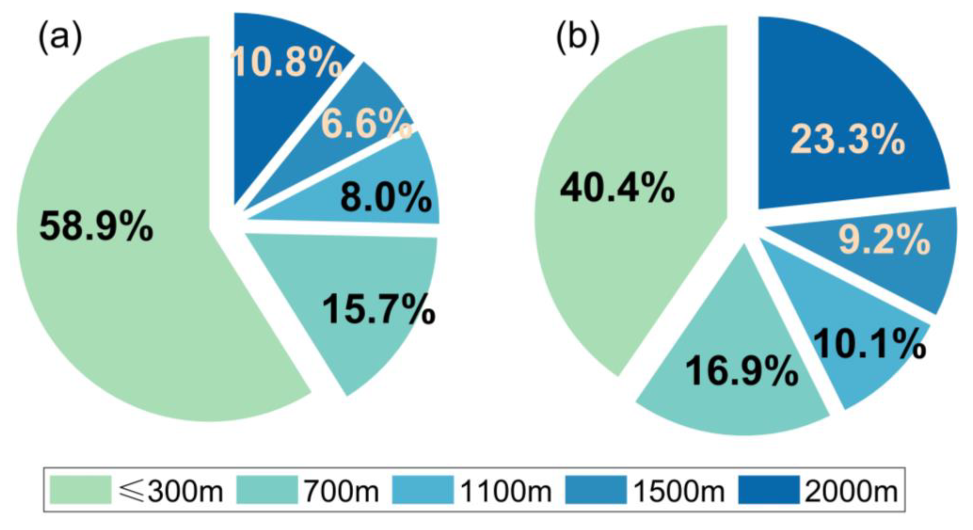
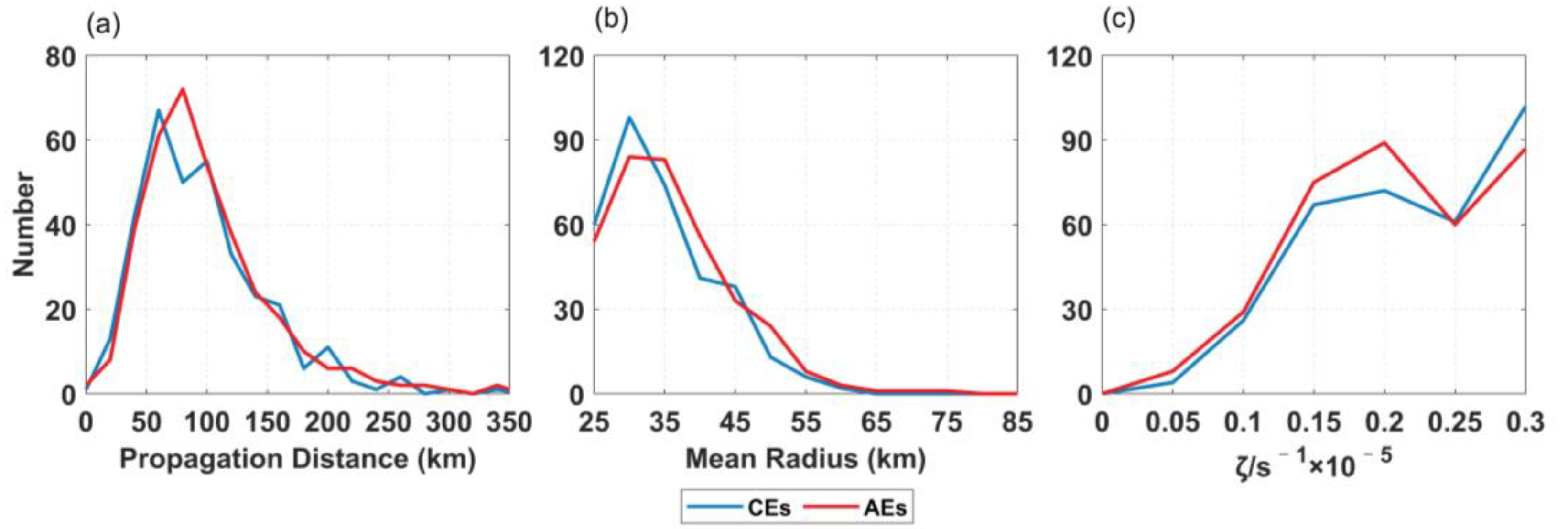
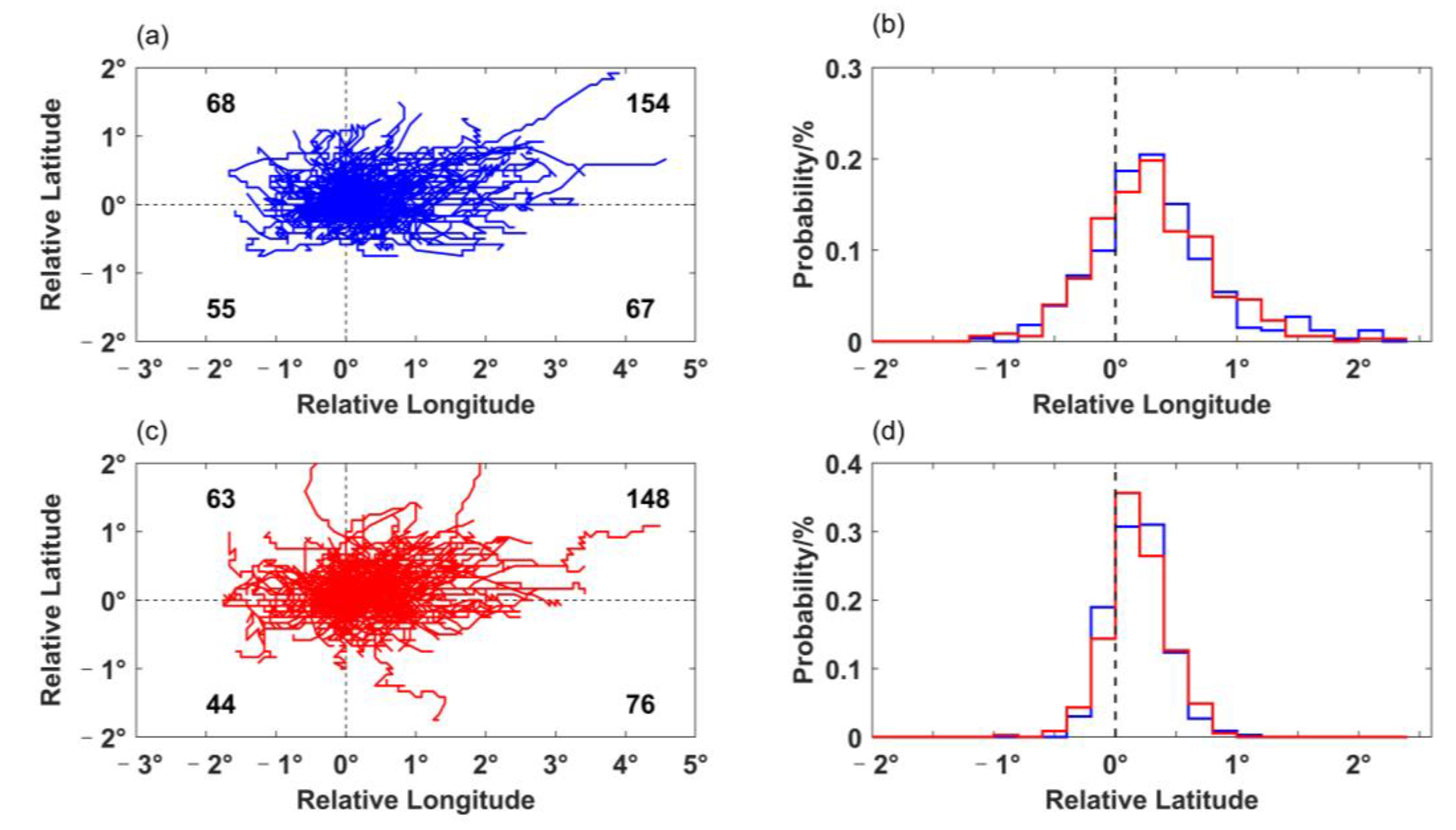
3.2. Eddy Radius, Voriticity and Propagation

A total of 680 eddies were detected using the 3D eddy detection method, with an average lifetime of 12.3 weeks and an average propagation distance of 97.8 km. The distribution of propagation distances peaks around 50–100 km, with 70.1% of the eddies having a propagation distance between 50 and 150 km (Figure 9a). The numbers of eddies with propagation distances greater than 50, 150 and 250 km are 575, 98 and 13, respectively. The average propagation distance of cyclones (96.7 km) is slightly smaller than that of anticyclones (98.9 km), with the number of cyclones slightly more than that of anticyclones for propagation distances of less than 60 km. However, the number of anticyclones becomes slightly more than that of cyclones as the propagation distance increases. The radius distribution of the cyclones and anticyclones are shown in Figure 9b. They range from 25 to 85 km with an average radius of 35.5 km, and are strongly skewed toward 25–45 km. Approximately 49.9% of the eddies are concentrated between 30 km and 35 km, while only 0.3% of the eddies have a radius greater than 65 km. The distribution of eddy radii is significantly skewed toward large values for anticyclonic eddies. For eddies with an average radius of 25 km to 30 km, there are more cyclones, while, for eddies with a larger radius, there are more anticyclones. The mean lifetime of cyclones (12.4 weeks) is almost same as that of anticyclones (12.2 weeks). For eddies with a lifetime of less than 10 weeks, there are 16 more anticyclones than cyclones. However, as the lifetime of the eddies increases, the difference between the number of cyclones and anticyclones becomes smaller, and, after more than 20 weeks, the number of cyclones slightly exceeds that of anticyclones. Regarding the absolute value of eddy vorticity, it is notable that 90.1% of eddies exhibit an absolute value of vorticity greater than 1.5 × 10⁻⁵ s⁻¹ (Figure 9c). The distribution of vorticity features two distinct peaks, occurring at 2 × 10⁻⁵ s⁻¹ and 3 × 10⁻⁵ s⁻¹, respectively. The average absolute value of vorticity for cyclones and anticyclones is 2.4 × 10⁻⁵ s⁻¹ and 2.2 × 10⁻⁵ s⁻¹, respectively. It is worth noting that more cyclones have vorticity values greater than 2.5 × 10⁻⁵ s⁻¹, while anticyclones typically have vorticity values of less than 2.5 × 10⁻⁵ s⁻¹.

It reveals that, in the Drake Passage, there is a positive correlation between eddy radius or vorticity and their lifetime, eddies with a larger radius or vorticity generally have a longer lifetime. Additionally, it appears that anticyclones tend to have longer propagation distances and larger mean radii than cyclones.

Mesoscale eddies are capable of transporting sea water during their movements, which, in turn, can affect the transport of various properties. The eddy propagation speed and direction are generally influenced by mean currents, and complex sea-air interactions can have an impact on the motion of eddies, too. Figure 10a,b illustrates the relative propagation trajectories of CEs and AEs, where both types of eddies start at the origin (0°N, 0°E), and their propagation trajectories are determined in relation to latitude and longitude, respectively. Generally, the average speed of eddies in the Drake Passage is 1.95 cm s⁻¹, and both cyclones and anticyclones have an average velocity of around 1.91 (1.98) cm s⁻¹. The propagation direction of most eddies is north-eastward for cyclones and anticyclones (Figure 10), accounting for 44.8% and 44.7%, respectively. The proportions of eddies in the other three quadrants are similar. Most eddies have propagation distances within 1 degree, consistent with Figure 9, while a few eddies can travel up to nearly 5 degrees. Both cyclones and anticyclones tend to move toward the equator, with cyclones accounting for 65% and anticyclones 64%. The mean zonal movement distances of CEs and AEs are 0.23 and 0.21 degrees, respectively, indicating the dominance of the eastward trend. This is inconsistent with previous research findings [41], which suggested that most cyclonic eddies move poleward, while most anticyclonic eddies move equatorward. In the zonal direction, both CEs and AEs move mainly westward within 50°S–50°N. The interactions between eddies and the Antarctic circumpolar current play a significant role in eddy movements in the Drake Passage, which is related to the flow direction of ACC as the background flow field. Compared with Kuroshio, eddies in the Drake Passage tend to have smaller propagation distances, shorter lifetimes and smaller radii. This is partly due to the fact that the latitude of Drake Passage is higher, and the Rossby deformation radius is smaller. It also because the Antarctic circumpolar current is a significant easterly flow with an average speed of less than 20 cm s⁻¹ [55], which offsets the westward movement caused by the combined effects of the $\beta$ effect and self-advection [41].

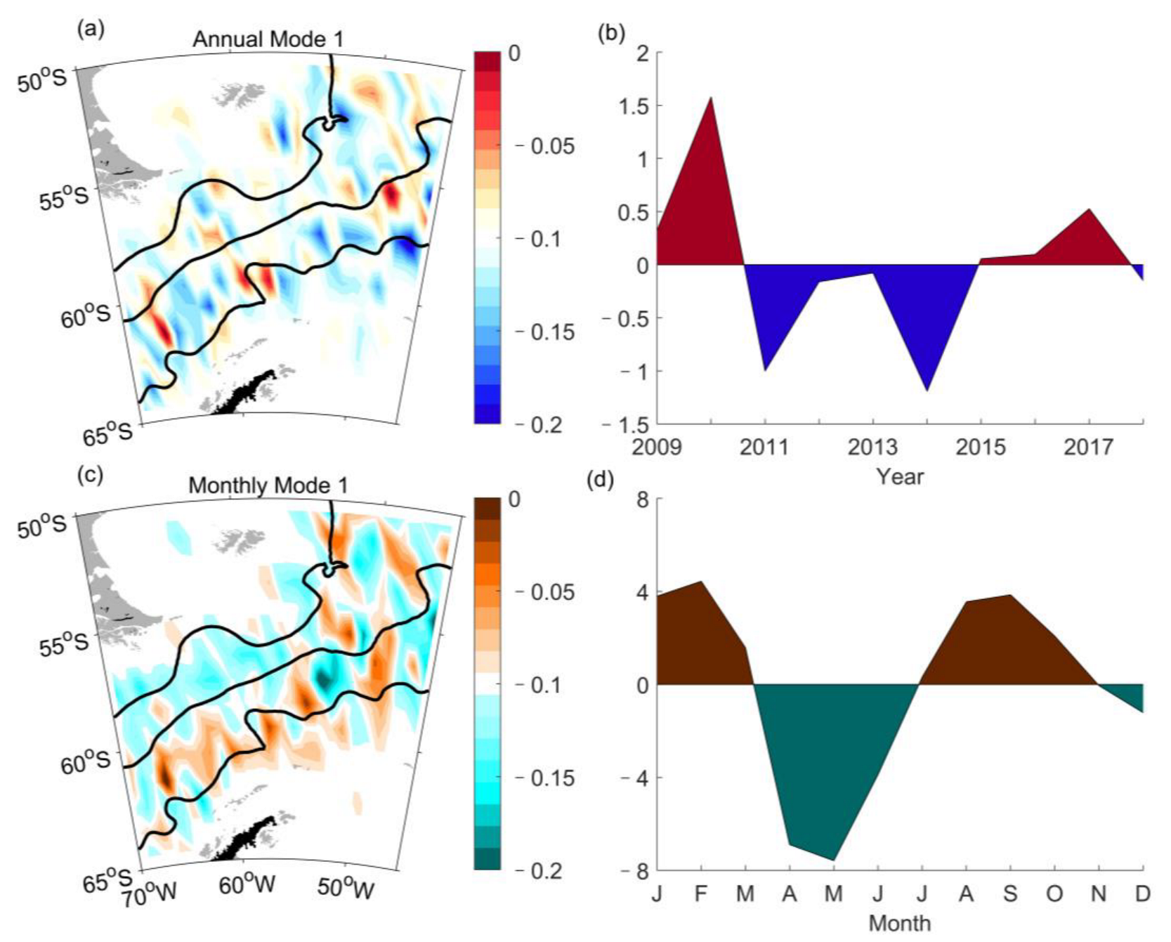
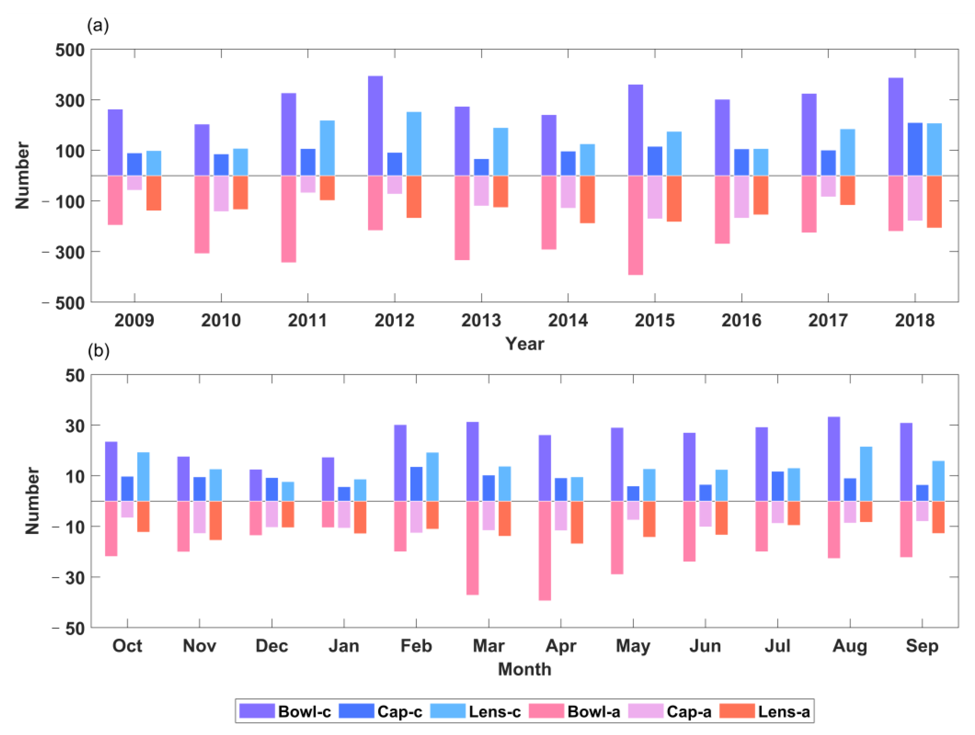
3.3. EOF Analysis of Eddy Annual and Monthly Variations

We utilized the EOF method to analyze the spatial and temporal variations of eddy numbers over 10 years (2009–2018) (Figure 11). Initially, we performed an EOF analysis of eddy numbers in a 1° × 1° grid to seek modes that correspond to the patterns and variation of time coefficients. Seven EOF modes are needed to represent 90% of the total variance. The first four EOFs accounted for 22.8%, 19.6%, 17.8% and 10.85% of the total variance and the spatial structures, respectively. The first EOF mode of both monthly and annual eddy numbers (Figure 11a,c) displays several standing eddies staggered in the south of SAF and the north of SACCF, which have a south-west–north-east direction, and are consistent with the positions of main fronts. In the annual distribution (Figure 11a), the eddies are particularly noticeable in significant fracture zones, such as the Endurance Fracture Zone (centered at 51°W, 57°S) and the Shackleton Fracture Zone (centered at 60°W, 59.5°S, as shown in Figure 1), where the frontal inflection is significant (consistent with Figure 7). For the principal components depicted in Figure 11b, the eddy numbers display significant interannual variations. In 2009, 2011, 2013 and 2015, the number of eddies was higher in the red area and lower in the blue area, and this variation decreases in magnitude over the years. The first mode pattern of the monthly eddy number variation exhibits more apparent spatial and temporal variations (Figure 11c,d). Take the PF as a boundary, the eddy numbers north and south of PF exhibit a seesaw pattern, with mainly positive values from October to February and June to August, indicating that eddy numbers increase in the south of the PF, especially in the Ona Basin, while they decrease north of the PF. From March to May, the pattern switches, with a decrease (increase) in eddy numbers in the south (north) of the PF.

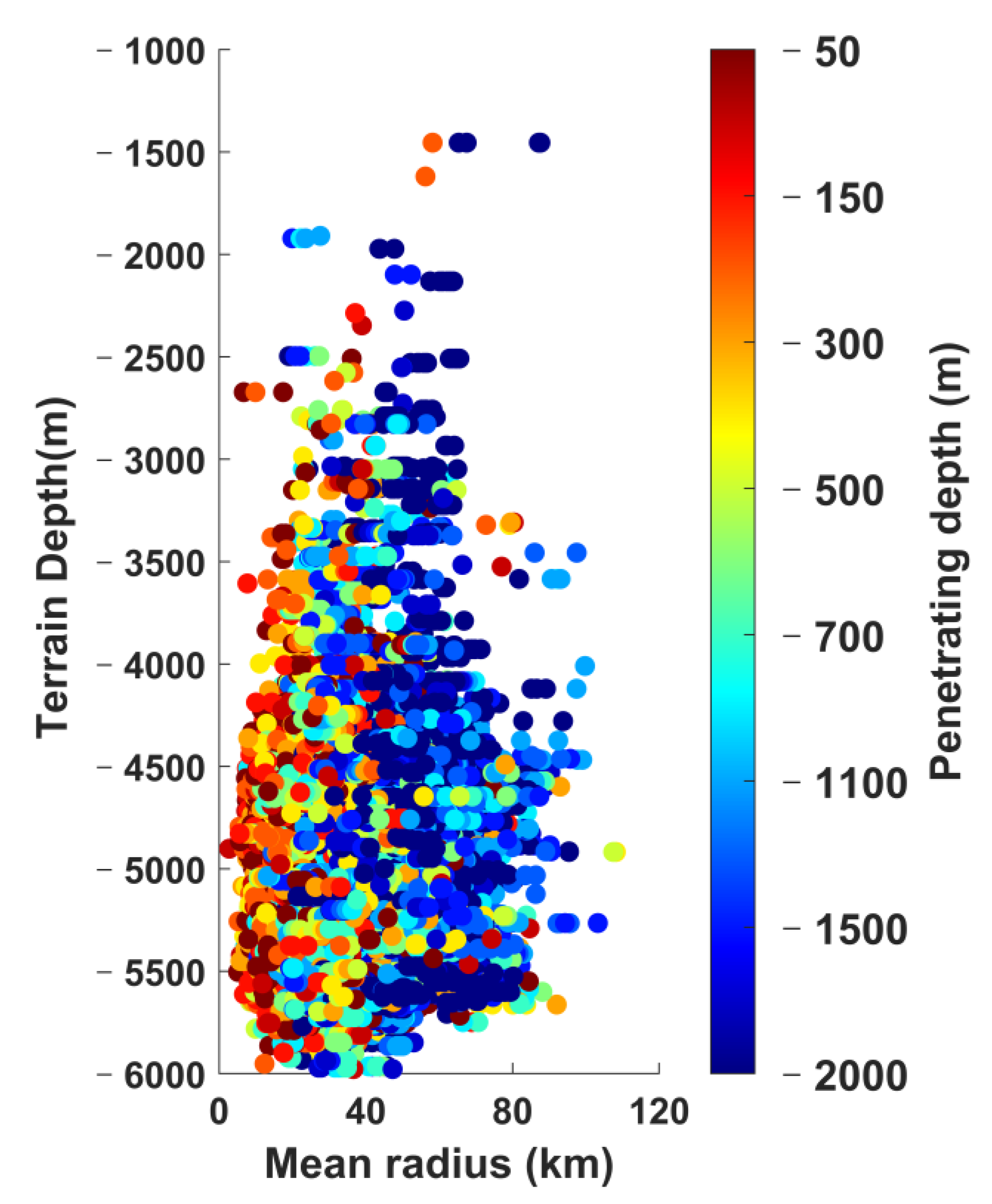
3.4. Eddy Variations with Water Depth

By examining the spatial distribution of the eddies (Figure 7a), it is apparent that the regions with the highest concentration of eddies are located in deeper waters, prompting us to investigate whether the activity of the eddies is related to the water depth of their locations. In this regard, we analyzed the eddy lifetime, mean radius, maximum radius, propagation distance and mean water depth at the location of the eddy. Figure 12 reveals that all the eddies in the Drake Passage with a mean radius larger than 25 km are distributed in waters deeper than 3500 m. This finding is consistent with previous research [56], which showed that eddies in the Southern Ocean are absent in water depths less than 2000 m. A significant portion (83%) of eddies in the Drake Passage are concentrated in water depths of 4500–5500 m water depth. Eddies with longer lifespans travel farther distances, and for eddies with a propagation distance greater than 300 km, their lifespan is typically greater than 25 weeks, and their average water depth is approximately 5500 m. However, no clear pattern exists between the lifespan of eddies and their average radius. From the relationship between the propagation distance and the average radius, the average radius of the more distant eddies ranges from 30 km to 50 km.

We conducted an analysis of the vertical characteristics of eddies, focusing on eddy numbers, average radius and lifespan with respect to water depth (Figure 13). The eddy number gradually decreases as the water depth increases. The highest number of eddies, totaling 734, is observed at a depth of 50 m. Above 400 m, the number of anticyclones slightly exceeds the number of cyclones, particularly at 50 m, where there are 40 more anticyclones than cyclones. Below 400 m, the difference in count between cyclones and anticyclones are negligible (Figure 13a). On average, the radius of anticyclones is slightly larger than cyclones, with the average radius decreasing with increasing water depth (Figure 13b). The mean radius of anticyclones across all depths, ranging from the surface to 2000 m, is 34.6 km (with a standard deviation of ±7.6 km), whereas for cyclones, it is 34.0 km (with a standard deviation of ±6.9 km). The largest average radius of anticyclones is found at around 400 m depth, where it is 1.5 km larger than cyclones. Beyond 900 m depth, the difference in average radius between cyclones and anticyclones is not significant, and at 1500 m the radius of cyclones is only 0.3 km larger than for anticyclones. However, the mean radius of anticyclones is still larger than for cyclones below 1500 m. The lifespan of eddies does not vary significantly with water depth, with an average lifespan of 12.8 weeks from the surface to 2000 m, and cyclones generally live longer than anticyclones (Figure 13c). This difference is more noticeable in the region above a depth of 400 m. Between 400 m and 900 m, the lifespans of the two types of eddies are comparable, but the standard deviation of anticyclones is slightly greater than that of cyclones. The lifespans of anticyclones are only longer than cyclones in the 900 m to 1500 m range, except at 1100 m, where the lifespan of cyclones is longer than anticyclones by up to 4.8 days.

Most eddies are found in regions where the water depths exceed 3500 m, with only a small percentage found in shallower waters (Figure 14). Eddies with a larger average radius are capable of reaching deeper depths. Eddies with radii smaller than 40 km can only penetrate to a maximum depth of 500 m. Eddies ranging from 40–80 km can penetrate to depths greater than 1500 m. Although the surface radius of the eddies is greater than 25 km, the average radius of these eddies at other depth is somewhat smaller, indicating that eddy shapes are different. Thus, further discussion is required to fully understand the three-dimensional structures of eddies.

According to previous research [53,54], three distinct three-dimensional eddy structures have been identified and named: bowl-shaped, cone-shaped and lens-shaped. Figure 15 displays three types of eddy shapes that each penetrating to a depth of 2000 m. The bowl-shaped anticyclone has a maximum radius of 28.2 km at surface and a minimum radius of 13.7 km at 1700 m. It has a warm core, with the warm anomaly extends down to 400 m. The tilting distance from eddy center in surface layer to the center in bottom layer is 5.3 km. The profiles of salinity anomaly and velocity also show significant anticyclone signals. The bowl-shaped cyclone has a maximum radius of 37.6 km at the surface, decreasing to a radius of 14.0 km at 2000 m. Its isotherm rises significantly, with a temperature anomaly greater than 0.5 °C compared to its surroundings. The center of this cold core is located at the surface and extends to a depth of 500 m, with a tilting distance of 5.5 km.

At a depth of 2000 m, the cone-shaped cyclone and anticyclone have maximum radii of 54.9 km and 55.3 km, respectively. The strongest warm temperature anomaly cores are between 300 to 800 m, with strong downwelling at the eddy center, and the velocity of the eddy boundary is 0.4 m s⁻¹. The upwelling of the cold- ore occurs up to 500 m, and the tilting distance of the cone-shaped anticyclone and cyclone are 4.9 km and 5.1 km, respectively.

The maximum radii of the lens-shaped anticyclone and cyclone are 47.9 km and 45.4 km, respectively, at depths of 1100 m and 900 m. The tilting distances of the other two eddies are 10.0 km and 5.2 km, respectively. The tilting distance of six cases ((a)–(e)) is around 5 km, which is consistent with previous results, and this is mainly due to their slow translation speed in each depth [51].

We categorized eddies that can penetrate to depths of 300, 700, 1100, 1500 and 2000 m into five groups. In each group, three types of three-dimensional eddy structures (bowl-shaped, cone-shaped and lens-shaped) are discussed. Figure 16 shows the variations in the number of these five groups of eddies. We found that the number of eddies with a penetrating depth of 2000 m is the largest, accounting for about 50% of all eddy snapshots, with 5822 cyclones snapshots and 5511 anticyclones snapshots. The number of eddies in the other four categories does not change much, with the total number of eddies varying between 2600 and 3200. Additionally, the number of anticyclones is slightly more than the number of cyclones in all other water depths except for eddies reaching 1500 m. For all five types of eddies at different water depths, bowl-shaped eddies are the most common (52.7%), followed by lens-shaped eddies (27.1%), and cap-shaped eddies are the least (20.2%), which is consistent with the findings in the western Pacific Ocean [57]. Moreover, for eddies reaching depths of 300 m and 700 m, the number of lens-shaped eddies and cone-shaped eddies were comparable, but for those deeper eddies, where the number of lens-shaped increased significantly compared to cone-shaped. Except for eddies reaching 2000 m depth, bowl-shaped eddies are more anticyclones than cyclones at all water depths.

Most of the Drake Passage eddies are small and can reach a depth of 2000 m. We explored the annual and monthly variations in the number of those eddies (Figure 17). On average, 1133 instantaneous eddies occur each year, but there is large interannual variability, with a minimum of 845 eddies in 2009 and a maximum of 1400 eddies in 2015. The number of cyclones and anticyclones varies significantly from year to year. The number of anticyclones was the smallest in 2009, with a count of 393, while the number of cyclones was the least in 2010, with a count of 398. In the years 2011–2012, and 2017–2018, there were more cyclones than anticyclones, with the highest number of cyclones occurring in 2018 with 806. While the rest of the years had fewer cyclones than anticyclones. The three types of eddies also show annual variations, with the largest number of bowl-shaped eddies occurring in 2015. Lens-shaped eddies had the highest number in 2012, with 421 (35%), while cone-shaped eddies had the highest number in 2018, with 389 (28%).

For the monthly variation, the total number of eddies is the lowest from March to April, and the highest from May to July. For other months, the number of eddies shows relatively little variation. Cyclones and anticyclones also exhibit monthly patterns, with more cyclones than anticyclones in five months, namely January, May and October to December. November has the highest number of cyclones with 641. Conversely, anticyclones dominate over cyclones in the remaining seven months, with July having the highest number of anticyclones at 680. In November, the difference in the number of cyclones and anticyclonic eddies was the largest, with 243 more cyclones than anticyclones, while, in September, the difference was the smallest, with 14 fewer cyclones than anticyclones. The three types of eddies exhibit distinct monthly trends, bowl-shaped eddies peak in June and reach their lowest point in March, while lens-shaped eddies peak in January, and have their lowest occurrence in March. Cone-shaped eddies show a peak in May and a trough in August. Overall, bowl-shaped eddies occur most frequently, followed by lens-shaped eddies and cone-shaped eddies. However, cone-shaped eddies are more prevalent than lens-shaped eddies in March.

4. Conclusions

Using 10 years of GLORYS12 Mercator Ocean reanalysis data (2009–2018), a three-dimensional statistical analysis of eddies in the Drake Passage was conducted. The accuracy of the GLORYS12 data was confirmed by comparing its results with satellite altimetry data and HYCOM model output, which showed good agreement with AVISO data. The surface spatial distribution and statistical characteristics of eddies were found to be consistent with Chelton’s eddy dataset. A 3D eddy dataset at 16 unevenly spaced vertical levels, ranging from the surface to 2000 m was obtained, including eddy temporal evolution of their characteristics, such as location, lifespan, radius, vorticity, propagation speed and distance. A total of 680 eddies, including 332 cyclones and 348 anticyclones, were detected for lifetime > 8 weeks and mean radius > 25 km. The mean lifespans of AEs and CEs were found to be 12.4 weeks and 12.2 weeks, respectively, with no significant difference between the two types of eddies from the surface to 2000 m. The average radius of eddies was 35.5 km, with about half of the eddies concentrated between 30–35 km, which is two to three times the baroclinic Rossby deformation radius. The variation of eddy radius with depth was found to be insignificant. The absolute value of vorticity for 90.1% of eddies was greater than 1.5 × 10⁻⁵ s⁻¹, with mean values of 2.4 × 10⁻⁵ s⁻¹ for cyclonic eddies and 2.2 × 10⁻⁵ s⁻¹ for anticyclonic eddies. Most of the eddies in the Drake Passage propagated north-eastward, influenced by the Antarctic Circumpolar Current, with an average propagation speed of 1.95 cm s-1 and average distance of 97.8 km. About 32.5% of eddies included 50% of eddy snapshots that penetrated deeper than 1000 m, and 23.3% reached a depth of 2000 m. Larger eddies were found to penetrate deeper, and were located over complex and deep-sea floor (>3500 m). Overall, anticyclones were found to be more prevalent from the surface to 400 m, exhibiting larger radius, and longer propagation distance, while cyclones had longer lifespans and greater vorticity. Between 400 and 2000 m, both anticyclones and cyclones demonstrated consistent values in terms of radius, lifetime and vorticity, but the anticyclones always have deeper penetration depth from surface to 2000 m.

Out of all eddies in the Drake Passage, 52.7% are bowl-shaped, and have the largest radius at the surface, followed by 27.1% lens-shaped eddies, with the largest radius at the middle-depth. The least common are cone-shaped eddies, with the largest radius at the eddy bottom. The occurrence of eddies in the Drake Passage varies annually and monthly, with more eddies in 2015 and fewer in 2009. Anticyclones outnumbered cyclones for four years (2011–2012 and 2017–2018), while cyclones outnumbered anticyclones for the remaining six years. For the monthly variation, the total number of eddies was the lowest from March to April and the highest from May to July. EOF analysis revealed significant annual eddy distribution in the Endurance Fracture Zone and the Shack Fracture Zone, while the monthly distribution of eddy number shows a seesaw pattern between the north and south of the PF. The Yaghan Basin is a region of cyclogenesis, and the Ona Basin is populated with deep-reaching eddies. The Drake Passage, located at high latitude with strong rotation and weak stratification, is more likely to generate small and deep-reaching eddies. These eddies are trapped by bottom topography; they do not propagate much, and their radius also not change too much. These deep-penetrating eddies not only affect the formation and ventilation of Antarctic intermediate water, but also interact with topography and induce turbulent dissipation modulation.

References

1. Provost, C.; Renault, A.; Barré, N.; Sennéchael, N.; Garçon, V.; Sudre, J.; Huhn, O. Two repeat crossings of Drake Passage in austral summer 2006: Short-term variations and evidence for considerable ventilation of intermediate and deep waters. Deep Sea Res. Part II Top. Stud. Oceanogr. 2011, 58, 2555–2571. [Google Scholar] [CrossRef]
2. Nowlin Jr, W.D.; Whitworth III, T.; Pillsbury, R.D. Structure and transport of the Antarctic Circumpolar Current at Drake Passage from short-term measurements. J. Phys. Oceanogr. 1977, 7, 788–802. [Google Scholar] [CrossRef]
3. Hofmann, E.E.; Whitworth III, T. A synoptic description of the flow at Drake Passage from year-long measurements. J. Geophys. Res. Ocean. 1985, 90, 7177–7187. [Google Scholar] [CrossRef]
4. Morrow, R.; Donguy, J.-R.; Chaigneau, A.; Rintoul, S.R. Cold-core anomalies at the subantarctic front, south of Tasmania. Deep. Sea Res. Part I Oceanogr. Res. Pap. 2004, 51, 1417–1440. [Google Scholar] [CrossRef]
5. Park, Y.H.; Park, T.; Kim, T.W.; Lee, S.H.; Hong, C.S.; Lee, J.H.; Rio, M.H.; Pujol, M.I.; Ballarotta, M.; Durand, I. Observations of the Antarctic Circumpolar Current over the Udintsev Fracture Zone, the narrowest choke point in the Southern Ocean. J. Geophys. Res. Ocean. 2019, 124, 4511–4528. [Google Scholar] [CrossRef]
6. Gutierrez-Villanueva, M.O.; Chereskin, T.K.; Sprintall, J. Upper-Ocean Eddy Heat Flux across the Antarctic Circumpolar Current in Drake Passage from Observations: Time-Mean and Seasonal Variability. J. Phys. Oceanogr. 2020, 50, 2507–2527. [Google Scholar] [CrossRef]
7. Meredith, M.P.; Woodworth, P.L.; Chereskin, T.K.; Marshall, D.P.; Allison, L.C.; Bigg, G.R.; Donohue, K.; Heywood, K.J.; Hughes, C.W.; Hibbert, A. Sustained monitoring of the Southern Ocean at Drake Passage: Past achievements and future priorities. Rev. Geophys. 2011, 49, RG4005. [Google Scholar] [CrossRef]
8. Joyce, T.; Patterson, S.; Millard, R., Jr. Anatomy of a cyclonic ring in the Drake Passage. Deep Sea Res. Part A Oceanogr. Res. Pap. 1981, 28, 1265–1287. [Google Scholar] [CrossRef]
9. Sprintall, J. Seasonal to interannual upper-ocean variability in the Drake Passage. J. Mar. Res. 2003, 61, 27–57. [Google Scholar] [CrossRef]
10. Barré, N.; Provost, C.; Sennechael, N.; Lee, J.H. Circulation in the Ona Basin, southern Drake Passage. J. Geophys. Res. Ocean 2008, 113, C04033. [Google Scholar] [CrossRef]
11. Bryden, H.L.; Heath, R.A. Energetic eddies at the northern edge of the Antarctic Circumpolar Current in the southwest Pacific. Prog. Oceanogr. 1985, 14, 65–87. [Google Scholar] [CrossRef]
12. Barré, N.; Provost, C.; Renault, A.; Sennéchael, N. Fronts, meanders and eddies in Drake Passage during the ANT-XXIII/3 cruise in January–February 2006: A satellite perspective. Deep Sea Res. Part II Top Stud. Oceanogr. 2011, 58, 2533–2554. [Google Scholar] [CrossRef]
13. Zhang, B.; Klinck, J.M. The effect of Antarctic Circumpolar Current transport on the frontal variability in Drake Passage. Dyn. Atmos. Ocean 2008, 45, 208–228. [Google Scholar] [CrossRef]
14. Lenn, Y.-D.; Chereskin, T.K.; Sprintall, J.; McClean, J.L. Near-surface eddy heat and momentum fluxes in the Antarctic Circumpolar Current in Drake Passage. J. Phys. Oceanogr. 2011, 41, 1385–1407. [Google Scholar] [CrossRef]
15. Trani, M.; Falco, P.; Zambianchi, E. Near-surface eddy dynamics in the Southern Ocean. Polar Res. 2011, 30, 11203. [Google Scholar] [CrossRef]
16. de Szoeke, R.A.; Levine, M.D. The advective flux of heat by mean geostrophic motions in the Southern Ocean. Deep Sea Res. Part A Oceanogr. Res. Pap. 1981, 28, 1057–1085. [Google Scholar] [CrossRef]
17. Frenger, I.; Münnich, M.; Gruber, N. Imprint of Southern Ocean mesoscale eddies on chlorophyll. Biogeosciences 2018, 15, 4781–4798. [Google Scholar] [CrossRef]
18. Kahru, M.; Mitchell, B.; Gille, S.; Hewes, C.; Holm-Hansen, O. Eddies enhance biological production in the Weddell-Scotia confluence of the Southern Ocean. Geophys. Res. Lett. 2007, 34, L14603. [Google Scholar] [CrossRef]
19. Korb, R.E.; Whitehouse, M. Contrasting primary production regimes around South Georgia, Southern Ocean: Large blooms versus high nutrient, low chlorophyll waters. Deep Sea Res. Part I Oceanogr. Res. Pap. 2004, 51, 721–738. [Google Scholar] [CrossRef]
20. Erickson, Z.K.; Thompson, A.F.; Cassar, N.; Sprintall, J.; Mazloff, M.R. An advective mechanism for deep chlorophyll maxima formation in southern Drake Passage. Geophys. Res. Lett. 2016, 43, 10846–10855. [Google Scholar] [CrossRef]
21. Jersild, A.; Delawalla, S.; Ito, T. Mesoscale Eddies Regulate Seasonal Iron Supply and Carbon Drawdown in the Drake Passage. Geophys. Res. Lett. 2021, 48, e2021GL096020. [Google Scholar] [CrossRef]
22. Bernard, A.; Ansorge, I.; Froneman, P.; Lutjeharms, J.; Bernard, K.; Swart, N. Entrainment of Antarctic euphausiids across the Antarctic Polar Front by a cold eddy. Deep Sea Res. Part I Oceanogr. Res. Pap. 2007, 54, 1841–1851. [Google Scholar] [CrossRef]
23. Hu, J.; Gan, J.; Sun, Z.; Zhu, J.; Dai, M. Observed three-dimensional structure of a cold eddy in the southwestern South China Sea. J. Geophys. Res. Ocean. 2011, 116. [Google Scholar] [CrossRef]
24. Zhang, Z.; Tian, J.; Qiu, B.; Zhao, W.; Chang, P.; Wu, D.; Wan, X. Observed 3D structure, generation, and dissipation of oceanic mesoscale eddies in the South China Sea. Sci. Rep. 2016, 6, 24349. [Google Scholar] [CrossRef]
25. He, Q.; Zhan, H.; Cai, S.; He, Y.; Huang, G.; Zhan, W. A new assessment of mesoscale eddies in the South China Sea: Surface features, three-dimensional structures, and thermohaline transports. J. Geophys. Res. Ocean. 2018, 123, 4906–4929. [Google Scholar] [CrossRef]
26. Qiu, C.; Liang, H.; Huang, Y.; Mao, H.; Yu, J.; Wang, D.; Su, D. Development of double cyclonic mesoscale eddies at around Xisha Islands observed by a ‘Sea-Whale 2000’autonomous underwater vehicle. Appl. Ocean. Res. 2020, 101, 102270. [Google Scholar] [CrossRef]
27. Liu, Z.; Liao, G.; Hu, X.; Zhou, B. Aspect ratio of eddies inferred from Argo floats and satellite altimeter data in the ocean. J. Geophys. Res. Ocean. 2020, 125, e2019JC015555. [Google Scholar] [CrossRef]
28. Petersen, M.R.; Williams, S.J.; Maltrud, M.E.; Hecht, M.W.; Hamann, B. A three-dimensional eddy census of a high-resolution global ocean simulation. J. Geophys. Res. Ocean. 2013, 118, 1759–1774. [Google Scholar] [CrossRef]
29. Cunningham, S.; Alderson, S.; King, B.; Brandon, M. Transport and variability of the Antarctic circumpolar current in drake passage. J. Geophys. Res. Ocean. 2003, 108. [Google Scholar] [CrossRef]
30. Jean-Michel, L.; Eric, G.; Romain, B.-B.; Gilles, G.; Angélique, M.; Marie, D.; Clément, B.; Mathieu, H.; Olivier, L.G.; Charly, R. The Copernicus global 1/12 oceanic and sea ice GLORYS12 reanalysis. Front. Earth Sci. 2021, 9, 698876. [Google Scholar] [CrossRef]
31. Lellouche, J.-M.; Le Galloudec, O.; Greiner, E.; Garric, G.; Regnier, C.; Drevillon, M.; Bourdallé-Badie, R.; Bricaud, C.; Drillet, Y.; Le Traon, P.-Y. The Copernicus Marine Environment Monitoring Service global ocean 1/12 physical reanalysis GLORYS12V1: Description and quality assessment. In Proceedings of the EGU General Assembly Conference Abstracts, Vienna, Austria, 8–13 April 2018; p. 19806. [Google Scholar]
32. Pujol, M.-I.; Faugère, Y.; Taburet, G.; Dupuy, S.; Pelloquin, C.; Ablain, M.; Picot, N. DUACS DT2014: The new multi-mission altimeter data set reprocessed over 20 years. Ocean Sci. 2016, 12, 1067–1090. [Google Scholar] [CrossRef]
33. Ezraty, R.; Girard-Ardhuin, F.; Piollé, J.-F.; Kaleschke, L.; Heygster, G. Arctic and Antarctic Sea Ice Concentration and Arctic Sea Ice Drift Estimated from Special Sensor Microwave Data; Département d’Océanographie Physique et Spatiale (IFREMER): Brest, France; University of Bremen: Bremen, Germany, 2007. [Google Scholar]
34. Cabanes, C.; Grouazel, A.; von Schuckmann, K.; Hamon, M.; Turpin, V.; Coatanoan, C.; Paris, F.; Guinehut, S.; Boone, C.; Ferry, N. The CORA dataset: Validation and diagnostics of in-situ ocean temperature and salinity measurements. Ocean Sci. 2013, 9, 1–18. [Google Scholar] [CrossRef]
35. Szekely, T.; Gourrion, J.; Pouliquen, S.; Reverdin, G.; Merceur, F. CORA, Coriolis Ocean Dataset for Reanalysis. 2019. Available online: https://www.seanoe.org/data/00351/46219/ (accessed on 13 January 2022).
36. Artana, C.; Ferrari, R.; Bricaud, C.; Lellouche, J.-M.; Garric, G.; Sennéchael, N.; Lee, J.-H.; Park, Y.-H.; Provost, C. Twenty-five years of Mercator ocean reanalysis GLORYS12 at Drake Passage: Velocity assessment and total volume transport. Adv. Space Res. 2021, 68, 447–466. [Google Scholar] [CrossRef]
37. Xia, Q.; Li, G.; Dong, C. Global Oceanic Mass Transport by Coherent Eddies. J. Phys. Oceanogr. 2022, 52, 1111–1132. [Google Scholar] [CrossRef]
38. Artana, C.; Provost, C.; Poli, L.; Ferrari, R.; Lellouche, J.M. Revisiting the Malvinas Current Upper Circulation and Water Masses Using a High-Resolution Ocean Reanalysis. J. Geophys. Res. Ocean. 2021, 126, e2021JC017271. [Google Scholar] [CrossRef]
39. Meng, Y.; Liu, H.; Lin, P.; Ding, M.; Dong, C. Oceanic mesoscale eddy in the Kuroshio extension: Comparison of four datasets. Atmos. Ocean. Sci. Lett. 2021, 14, 100011. [Google Scholar] [CrossRef]
40. Chelton, D.B.; Schlax, M.G.; Samelson, R.M. Global observations of nonlinear mesoscale eddies. Prog. Oceanogr. 2011, 91, 167–216. [Google Scholar] [CrossRef]
41. Fu, L.-L.; Chelton, D.B.; Le Traon, P.-Y.; Morrow, R. Eddy dynamics from satellite altimetry. Oceanography 2010, 23, 14–25. [Google Scholar] [CrossRef]
42. Okubo, A. Horizontal dispersion of floatable particles in the vicinity of velocity singularities such as convergences. Deep Sea Res. Oceanogr. Abstr. 1970, 17, 445–454. [Google Scholar] [CrossRef]
43. Weiss, L.A. Bankruptcy resolution: Direct costs and violation of priority of claims. J. Financ. Econ. 1990, 27, 285–314. [Google Scholar] [CrossRef]
44. Chaigneau, A.; Gizolme, A.; Grados, C. Mesoscale eddies off Peru in altimeter records: Identification algorithms and eddy spatio-temporal patterns. Prog. Oceanogr. 2008, 79, 106–119. [Google Scholar] [CrossRef]
45. Nencioli, F.; Dong, C.; Dickey, T.; Washburn, L.; McWilliams, J.C. A vector geometry–based eddy detection algorithm and its application to a high-resolution numerical model product and high-frequency radar surface velocities in the Southern California Bight. J. Atmos. Ocean. Technol. 2010, 27, 564–579. [Google Scholar] [CrossRef]
46. Cui, W.; Wang, W.; Zhang, J.; Yang, J. Identification and census statistics of multicore eddies based on sea surface height data in global oceans. Acta Oceanol. Sin. 2020, 39, 41–51. [Google Scholar] [CrossRef]
47. Xing, T.; Yang, Y. Three mesoscale eddy detection and tracking methods: Assessment for the South China Sea. J. Atmos. Ocean. Technol. 2021, 38, 243–258. [Google Scholar] [CrossRef]
48. Chen, G.; Hou, Y.; Chu, X. Mesoscale eddies in the South China Sea: Mean properties, spatiotemporal variability, and impact on thermohaline structure. J. Geophys. Res. Ocean. 2011, 116, C06018. [Google Scholar] [CrossRef]
49. Mkhinini, N.; Coimbra, A.L.S.; Stegner, A.; Arsouze, T.; Taupier-Letage, I.; Béranger, K. Long-lived mesoscale eddies in the eastern Mediterranean Sea: Analysis of 20 years of AVISO geostrophic velocities. J. Geophys. Res. Ocean. 2014, 119, 8603–8626. [Google Scholar] [CrossRef]
50. Schaeffer, A.; Gramoulle, A.; Roughan, M.; Mantovanelli, A. Characterizing frontal eddies along the East Australian Current from HF radar observations. J. Geophys. Res. Ocean. 2017, 122, 3964–3980. [Google Scholar] [CrossRef]
51. Wang, X.; Zhang, S.; Lin, X.; Qiu, B.; Yu, L. Characteristics of 3-Dimensional Structure and Heat Budget of Mesoscale Eddies in the South Atlantic Ocean. J. Geophys. Res. Ocean. 2021, 126, e2020JC016922. [Google Scholar] [CrossRef]
52. Dong, C.; Lin, X.; Liu, Y.; Nencioli, F.; Chao, Y.; Guan, Y.; Chen, D.; Dickey, T.; McWilliams, J.C. Three-dimensional oceanic eddy analysis in the Southern California Bight from a numerical product. J. Geophys. Res. Ocean. 2012, 117, C00H14. [Google Scholar] [CrossRef]
53. Lin, X.; Dong, C.; Chen, D.; Liu, Y.; Yang, J.; Zou, B.; Guan, Y. Three-dimensional properties of mesoscale eddies in the South China Sea based on eddy-resolving model output. Deep Sea Res. Part I Oceanogr. Res. Pap. 2015, 99, 46–64. [Google Scholar] [CrossRef]
54. Qiu, C.; Yi, Z.; Su, D.; Wu, Z.; Liu, H.; Lin, P.; He, Y.; Wang, D. Cross-Slope Heat and Salt Transport Induced by Slope Intrusion Eddy’s Horizontal Asymmetry in the Northern South China Sea. J. Geophys. Res. Ocean. 2022, 127, e2022JC018406. [Google Scholar] [CrossRef]
55. Klinck, J.; Nowlin, W. Antarctic Circumpolar Current. In Encyclopedia of Ocean Sciences; Steele, J., Thorpe, S., Turekian, K., Eds.; Academic Press: Cambridge, MA, USA, 2001; Volume 151, p. 159. [Google Scholar]
56. Frenger, I.; Münnich, M.; Gruber, N.; Knutti, R. Southern Ocean eddy phenomenology. J. Geophys. Res. Ocean. 2015, 120, 7413–7449. [Google Scholar] [CrossRef]
57. Yang, G.; Lin, X.; Han, G.; Liu, Y.; Chen, G.; Wang, J. Three-dimensional characteristics of mesoscale eddies simulated by a regional model in the northwestern Pacific Ocean during 2000–2008. Acta Oceanol. Sin. 2022, 41, 74–93. [Google Scholar] [CrossRef]
Figure 1. Bottom topography (m) of the Drake Passage. Black thick lines represent the climatological location of the major ACC fronts. Park et al. [5] have made the data on the geographical locations of five altimetry-derived fronts of the Antarctic Circumpolar Current available for open access. The data can be downloaded from https://www.seanoe.org/data/00486/59800/. From north to south: the Subantarctic Front (SAF), the Polar Front (PF) and the Southern ACC front (SACCF). The SAF and PF exit the Drake Passage and enter the Argentine Basin. The main basins in the Drake Passage are: the Former Phoenix Plate Basin (FPPB), the Yaghan Basin (YB), the Ona Basin (OB) and the Northeast Scotia Sea Basin (NESSB). The EFZ and SFZ represent the Endurance Fracture Zone and the Shackleton Fracture Zone, respectively. The 2000 m isobaths are represented by thick gray lines.
Remotesensing 15 02462 g001
Figure 2. Mean eddy kinetic energy (EKE, cm2 s−2) calculated from gridded surface geostrophic current anomalies during 2009–2018. (a) AVISO; (b) HYCOM; and (c) GLORYS12. The three black thick lines are the climatological location of three main fronts.
Remotesensing 15 02462 g002
Figure 3. The vertical distribution of area-averaged eddy kinetic energy (EKE), along with their corresponding standard deviations. The orange lines and shades are from HYCOM data, while the purple ones represent GLORYS12′s result. At the surface, the mean EKE values calculated from AVISO, GLORYS12 and HYCOM are represented by blue, purple and orange points, respectively.
Remotesensing 15 02462 g003
Figure 4. (a) The vertical distribution of area-averaged annual mean temperature. The black and red lines are vertical annual mean temperature from the Argo and GLORYS12 dataset, respectively. (b) The vertical sections of temperature along 57.5°S (the median latitude of the study area) from the Argo data, (c) are the same as (b), but the data is from GLORYS12. The Argo data was downloaded from https://argo.ucsd.edu/data/argo-data-products/, accessed on 2 May 2023.
Remotesensing 15 02462 g004
Figure 5. Snapshots of the eddy distribution on the same date (6th November, 2010). (a) AVISO; (b) GLORYS12; (c) HYCOM. The quivers represent velocity directions and colors are the absolute velocity.
Remotesensing 15 02462 g005
Figure 6. (a) The spatial distribution of eddies with radius greater than 25 km and lifespan greater than 8 weeks obtained using GLORYS12 model; (b) results from “Mesoscale Eddy Trajectory Atlas” product. The variation of eddy number with lifespan obtained by different datasets: (c) eddy number varied with different lifespans from GLORYS12 data and (d) the Chelton dataset.
Remotesensing 15 02462 g006
Figure 7. Ratio distribution of eddies production sites in a 1° × 1° grid for various lifespan ranges and corresponding distribution of eddies polarity: (a) distribution of eddy with an average lifespan of less than 8 weeks; (b) eddy with average lifetime of longer than 8 weeks; (c) the distribution of eddy polarities with a lifespan of fewer than 8 weeks; (d) is the same as (c), but for lifespans of more than 8 weeks. The orange bins indicate a higher count of anticyclones compared to cyclones; the blue bins represent a higher count of cyclones over anticyclones.
Remotesensing 15 02462 g007
Figure 8. Distribution of penetrating depth for eddies detected using the 3D eddy detection method. (a) The penetrating depth distribution of original eddies without any thresholds; (b) the penetrating depth distribution of eddies with the applied thresholds, i.e., eddies with lifespans greater than 8 weeks and mean radii greater than 25 km. The percentages represent the proportion of eddies at different penetration depths, with a black font for those less than 1000 m and gray and white fonts for those exceeding 1500 m.
Remotesensing 15 02462 g008
Figure 9. The number of eddies varied with eddy parameters during their lifespans. (a) Propagation distance, (b) average radius, (c) absolute value of vorticity.
Remotesensing 15 02462 g009
Figure 10. The deflections and average displacement of propagation trajectories. (a) Propagation trajectories of all CEs from their initial positions (set as 0°N, 0°E). (b) Same as (a) but for all AEs. Negative changes in longitude (latitude) indicate westward (poleward) movement, while positive changes in longitude and latitude represent eastward and equatorward, respectively. The histograms on the right panels show the average movement of each eddy trajectory along (c) longitude and (d) latitude. The blue and red lines represent CEs and AEs, respectively.
Remotesensing 15 02462 g010
Figure 11. EOF analysis of eddy numbers in 1° × 1° grid and their corresponding time coefficients. (a) The first EOF mode of the annual eddy numbers; (b) the corresponding principal components. (c,d) are similar to (a,b), respectively, but for monthly eddy numbers. The three thick black lines from north to south represent SAF, PF and SACCF, respectively.
Remotesensing 15 02462 g011
Figure 12. (a) The water depth where eddies occur and the relationship between their lifespan and propagation distance; (b) similar to (a), the relationship between water depth and eddy lifespan and mean radii; (c) the relationship between the maximum radius of eddies and their lifespans and propagation distance; (d) the relationship between the mean radius of eddies and their lifespans and propagation distance.
Remotesensing 15 02462 g012
Figure 13. Eddy parameters varied with water depth. (a) Eddy number; (b) mean radius; (c) mean lifetime. The blue lines are the mean values of cyclones, and the red dashed line represents the mean values of anticyclones. The blue and red patches represent the standard deviations of cyclones and anticyclones, respectively.
Remotesensing 15 02462 g013
Figure 14. Distribution of mean radius and penetrating depth of eddies varied with water depth. The color represents eddy penetrating depth.
Remotesensing 15 02462 g014
Figure 15. The three types of eddies with distinct vertical structures. (a) The bowl-shaped cyclones (anticyclones) and their temperature, salinity anomaly and velocity along longitude through eddy center; (b) same as (a), but with examples of cone-shaped cyclones (anticyclones); (c) lens-shaped cyclones (anticyclones). The thick black solid lines denote the eddy centers, while the dashed black lines are contours representing the outermost enclosed streamlines surrounding these centers, thus, delineating the eddy boundaries.
Remotesensing 15 02462 g015aRemotesensing 15 02462 g015b
Figure 16. The number of different three-dimensional structures for different water depth eddies. Dark blue (orange) circles represent bowl-shaped anticyclonic (cyclonic) eddies, yellow (purple) diamonds represent cone-shaped anticyclonic (cyclonic) eddies and green (light blue) squares are lens-shaped anticyclones (cyclones).
Remotesensing 15 02462 g016
Figure 17. (a) Annual and (b) monthly variation of three different structures of eddies reaching depths of 2000 m. The purple, dark blue and light blue bars represent bowl-shaped, cone-shaped and lens-shaped cyclones, respectively. The magenta, pink and orange bars represent anticyclones with different 3D structures.
Remotesensing 15 02462 g017
Disclaimer/Publisher’s Note: The statements, opinions and data contained in all publications are solely those of the individual author(s) and contributor(s) and not of MDPI and/or the editor(s). MDPI and/or the editor(s) disclaim responsibility for any injury to people or property resulting from any ideas, methods, instructions or products referred to in the content.