Article

Sea Surface pCO2 Response to Typhoon “Wind Pump” and Kuroshio Intrusion in the Northeastern South China Sea

1
State Key Laboratory of Tropical Oceanography, South China Sea Institute of Oceanology, Chinese Academy of Sciences, Guangzhou 510301, China
2
Guangdong Remote Sensing Center for Marine Ecology and Environment (GDRS), Southern Marine Science and Engineering Guangdong Laboratory (Guangzhou), Guangzhou 511458, China
3
South China Sea Development Research Institute, Ministry of Natural Resources, Guangzhou 510300, China
4
University of Chinese Academy of Sciences, Beijing 100049, China
*
Author to whom correspondence should be addressed.
Remote Sens. 2024, 16(1), 123; https://doi.org/10.3390/rs16010123
Submission received: 1 December 2023 / Revised: 20 December 2023 / Accepted: 21 December 2023 / Published: 27 December 2023

Abstract

:
The Luzon Strait (LS) is a key region for estimating carbon sources and sinks in the South China Sea (SCS) and is highly influenced by the Kuroshio Current (KC) and typhoons. Understanding the variations in the sea surface partial pressure of carbon dioxide (pCO2-sw) under the combined effects of typhoons and KC in this region is crucial for estimating local and regional changes in ocean carbon flux. Based on valuable in situ pCO2-sw and remote sensing data, this study aimed to reveal the temporal variations and the physical mechanisms of pCO2-sw variations under the comprehensive effects of both typhoons and Kuroshio Intrusion (KI) in the LS. One week after the passage of the tropical cyclone (TC) Nanmadol, the concentration in the pCO2-sw and the influencing mechanisms varied in three different regions (W1–W3) on Transect A (120°E). In the region dominated by SCS waters (W1), the average pCO2-sw increased by 5.1 μatm after TC, which was mainly due to the TC “Wind Pump” inducing strong vertical mixing, which brought dissolved inorganic carbon (DIC)-rich deeper water up to the surface. In the region affected by KC (W2 and W3), pCO2-sw decreased after the TC (−8.2 μatm and −1.8 μatm, respectively) with TC-enhanced KI because the invasion of lower pCO2-sw of Kuroshio waters inhibited the TC-induced upwelling. More significant TC-induced upwelling (W3) would alleviate the decrease in pCO2-sw caused by the TC-enhanced KI. This study is a rare case providing a better understanding of the variations in pCO2-sw under TC-enhanced KI, which provides support for regional climate change prediction and carbon flux estimation in the western boundary current regions.

1. Introduction

The sea surface partial pressure of carbon dioxide (pCO2-sw) is an intermediate factor of sea–air carbon dioxide exchange and plays a vital role in the transportation of carbon from the ocean surface to deeper layers [1]. The pCO2-sw is determined by four primary factors, temperature, dissolved inorganic carbon (DIC), total alkalinity, and salinity [2]. The concentration and distribution of pCO2-sw are affected by multiple biological, chemical, and physical processes [2,3].
The South China Sea (SCS) is an essential part of the global ocean carbon cycle and generally acts as a carbon source for atmospheric CO2, and the carbon source–sink pattern presents temporal and spatial disparities [4,5,6,7]. In the northern SCS, it acts as a carbon source in the summer and autumn [8]. Among the northern SCS, the Luzon Strait (LS), as the boundary between the SCS and the Pacific Ocean, is also a typical western boundary current region [9]. The unique geographical environments and circulation processes make it a highly representative area in the SCS. The variations in pCO2-sw also exhibit regional characteristics over the LS.
A high frequency of typhoon activities occurs in the northeastern South China Sea (NESCS), especially over the LS. Previous studies have shown that typhoon “Wind Pump” have a significant impact on the physical and biochemical environment of the upper ocean, including causing a decrease in sea surface temperature (SST), an increase in sea surface salinity (SSS), an increase in surface or subsurface phytoplankton biomasses, an increase in dissolved oxygen (DO), etc. [10,11,12,13,14,15,16,17,18,19]. Typhoon “Wind Pump” also induce dynamic ocean processes, such as upwelling, vertical mixing, eddies, and fronts. Variations in these physical and biochemical processes may affect the concentration of pCO2-sw. The degree of influence is determined by the typhoon’s intensity, moving path, moving speed, precipitation, and the combined effects of the marine environment and other factors [14,15,16,17,20,21,22,23,24]. Nemoto et al. (2009) discovered that three typhoons were responsible for approximately 60% of the CO2 emissions during the summer season in the western subtropical North Pacific. The variation in pCO2-sw was likely influenced by the vertical mixing and upwelling caused by the typhoons [20]. Sun et al. (2014) found that the passage of a TC over the SCS turned a sink for atmospheric CO2 into a source. The undersaturation of CO2 prior to the TC due to dilution by freshwater and the preexisting cold eddy and the slow translation speed of the TC were the influencing mechanisms for the CO2 flux change [16]. Ye et al. (2017) examined the typhoon-induced changes in pCO2-sw and CO2 flux in the SCS and corroborated the previous conclusion that the local air–sea CO2 flux was affected significantly by oceanographic conditions during the typhoon [17]. Yu et al. (2020) studied the changes in pCO2-sw and carbon flux before and after three typhoons in the northern SCS and proposed three processes through which typhoons could affect pCO2-sw, which were cooling, vertical mixing, and upwelling. Typhoons were found to cause an average increase in the air–sea CO2 flux that ranged from 3.6 to 5.4 times the pre-typhoon flux [21]. Kao et al. (2023) revealed a significant decrease in pCO2-sw following typhoon Maria in the upwelling region in the southern East China Sea (ECS), both on the shelf break and middle shelf. Among the controlling factors, the effect of temperature accounted for 38% to 40%, net biological activity −33% to −36%, and mixing −24% [22].
In addition, the horizontal transport process of Kuroshio water will also affect the concentration of pCO2-sw, modifying the regional ocean carbon cycle [7,25,26,27]. Tsao et al. (2023) studied 9 years of measured pCO2-sw data for the Kuroshio Current (KC) in the eastern ECS and found that the rapidly warming KC may have led to an increasing trend in pCO2-sw [25]. Li et al. (2022) investigated the latitudinal changes in pCO2-sw and air–sea partial pressure difference (ΔpCO2) in the Kuroshio extension (KE) area on the northwest side of the North Pacific and found that northward cooling and vertical mixing were the two main processes controlling the latitudinal gradients of surface pCO2-sw and ΔpCO2, while biological influences were relatively minor [28]. Chou et al. (2007) studied the transport of subsurface water in the SCS, including pH, DIC, TA, and other factors, and proved that Kuroshio could considerably change its water properties in its onshore flank due to the SCS subsurface outflow as it bypassed the LS [27].
Fan et al. (2022) investigated how pCO2-sw responded to both typhoons Saola and Kuroshio in eastern Taiwan Island in 2012. Significant changes in the horizontal transport pattern of Kuroshio water were observed before and after the typhoon, which played a crucial role in controlling pCO2-sw. The deepening of the mixed layer after typhoons had less of an impact on pCO2-sw due to the offsetting effects of increased salinity and DIC input from the lower layer [29].
In summary, the impacts of typhoons or Kuroshio on pCO2-sw have been documented by several studies. However, few studies have explored the changes in pCO2-sw under the combined effects of typhoons and Kuroshio in LS, as it is hard to obtain in situ data in extreme weather, such as typhoons. In this study, we obtained in situ pCO2 data after the typhoon over the LS region where enhanced Kuroshio Intrusion (KI) was found in September 2011. These valuable data provided an opportunity for further revealing the change in pCO2-sw under extreme weather conditions.
Based on the in situ measurements and remote sensing data, this study analyzes the variations in pCO2-sw before and after the TC in three different regions along the LS, and reveals their possible mechanisms under the comprehensive effects of a typhoon “Wind Pump” and KI in the NESCS. This study may contribute to a better understanding of the variations in air–sea carbon fluxes under TC-enhanced KI and provides support for regional climate change prediction and carbon flux estimation in the western boundary current regions.
This study is structured as follows: The background is provided in Section 1. Data and methods are provided in Section 2. The results of the variations in pCO2-sw and other related parameters are provided in Section 3. Discussions of the possible mechanisms of pCO2-sw variations under the combined effects of the typhoon “Wind Pump” and KI in three defined regions are provided in Section 4. Conclusions are provided in Section 5.

2. Data and Methods

2.1. Typhoon Track Data

The typhoon or tropical cyclone (TC)’s track data were acquired from the Joint Typhoon Warning Center. They consisted of 6-hourly time series of the typhoon’s center locations, maximum sustained wind speed (MSW) at a height of 10 m above the mean sea level, satellite imagery, and the TC status. The velocity of the typhoon was estimated by calculating the change in the position of its center over time. On 22 August in 2011, the TC Nanmadol generated in the western Pacific Ocean as a tropical depression. Subsequently, the TC gradually strengthened into a tropical storm and altered its trajectory toward the northwest. On 27 August, it arrived at the LS with a MSW of 110 m/s. The TC passed the LS from 00:00 UTC on 27 August to 18:00 UTC on 28 August, with an average transition velocity of 2.9 m/s. The TC weakened to a tropical storm after it passed Taiwan Island and finally made landfall at 00:00 UTC on 31 August (Figure 1).

2.2. In Situ Data

The cruise data were obtained from the research vessel Shiyan 3 in the SCS. The cruise, organized by the South China Sea Institute of Oceanology, Chinese Academy of Sciences, was conducted from 19 August to 12 September 2011. In this study, we focus on the data from approximately one week following the passage of the TC in Transect A (120°E, 19.5°N to 21.5°N, 3 September to 4 September in 2011).

2.2.1. The pCO2

An automated flowing pCO2 measuring system (GO8050), widely used for measuring pCO2-sw on ships and other at-sea platforms, was utilized to collect data on pCO2-sw and atmospheric pCO2 (pCO2-air) [5]. The pCO2-sw was measured for 70 s/record, and the pCO2-sw records were averaged over a period of 3 min. It was measured every 2 h in air pumped from a bow intake located at the prow, situated 10 m above the water’s surface. In the system, a LICOR nondispersive infrared spectrometer was used to measure dried CO2 fractions (xCO2) in the equilibrator and in the air [5]. This system continuously monitored the pressure and temperature inside the main balancer. By using measurements of sea surface temperature and salinity, along with all the parameters obtained by the system, it was possible to calculate the effective pressure of both seawater and the surface atmosphere. After a series of calculations and adjustments, the pCO2-sw could be obtained. The saturated water vapor pressure and the temperature effect coefficient of 4.23%_C−1 were used to calculate the in situ pCO2-sw [2]. The standard error between standard gases and measured values was less than 1% [5,16].
We compared the in situ data with the recent research to ensure the reliability of the data. In the region near the LS, the range of the pCO2-sw was 360–380 μatm in September, which was close to the equilibrium with the atmosphere and consistent with the previous research [26,28,30].
Surface Ocean CO2 Atlas (SOCAT) is a database that provides access to quality-controlled, in situ measurements of pCO2-sw. SOCAT data are collected from a range of sources, including research cruises, moored buoys, and autonomous platforms, and undergo rigorous quality control procedures to ensure accuracy and consistency. The database includes variables such as latitude, longitude, time, temperature, salinity, and pCO2, allowing researchers to analyze and model the carbon dioxide dynamics in the surface ocean. Data from Jan 2008 to April 2009 could be found within the area of 118–122°E and 15–25°N, which were used to calculate the background level of pCO2-sw in our study area.

2.2.2. SST and SSS

During the entire cruise, seawater was continuously extracted from a bow intake positioned 5 m below the sea surface: SST and SSS were measured and recorded at a frequency of every 5 s using a Seabird CTD (SBE21, Sea-Bird Scientific, Bellevue, WA, USA), and the records were averaged over a period of 3 min.

2.2.3. ADCP Current

An acoustic Doppler current profiler (ADCP) was employed to determine the speed and direction of the ocean currents at various depths. Current profiles were obtained at intervals of 16 m starting from a depth of 38 m and extending down to a depth of 500 m.

2.2.4. Argo Floats

In this study, observations obtained from Argo floats were utilized to analyze the temporal variations in temperature and salinity within the upper layer of the western LS during the passage of Nanmadol in 2011. Two Argo floats, named Argo1 and Argo2, were identified in close proximity to the LS and Transect A (Figure 1). The potential temperature, salinity, and potential density of the two Argo floats from 5–200 m were employed to investigate the vertical hydrographic responses to Nanmadol in the upper ocean.

2.3. Satellite Data and Model Data

2.3.1. Satellite Data

The near-surface wind field, characterized by a spatial resolution of 25 km, was retrieved from data of the Advanced Scatterometer (ASCAT) onboard the European MetOp satellite. The SST data (8-day composites with 4 km resolution) were derived from data of the Moderate-Resolution Imaging Spectroradiometer (MODIS) onboard the Aqua satellite. The sea level anomaly (SLA) data were retrieved from the AVISO website with a spatial resolution of 1/3° × 1/3° and a temporal resolution of 7 days. The SLA data were merged from the radar altimeters onboard the ERS1/2, TOPEX/Poseidon, and Jason satellites. The weekly precipitation data were computed using the daily data acquired from the ASCAT dataset, with a spatial resolution of 0.25° × 0.25°.

2.3.2. HYCOM Data

The HYCOM + NCODA data, with a resolution of 1/12°, were retrieved on a Mercator grid between 80.48°S and 80.48°N (1/12° equatorial resolution), which had 40 vertical layers. Weekly three-dimensional potential temperature, salinity, and current data were calculated from the daily data produced by this HYCOM + NCODA Global 1/12° Analysis (GLBa0.08) (http://hycom.org/dataserver/glb-analysis, accessed on 20 December 2023).
All the above data were listed in Table 1.

2.4. Method

2.4.1. Calculation of Normalized pCO2

To examine the effects of factors other than temperature on the variation in pCO2-sw, pCO2-sw was normalized as NpCO2 using the mean SST as follows:
N p CO 2 = p CO 2 sw exp ( 0.0423 Tobs Tmean )
where T represents the SST, Tmean represents the mean SST during the entire observation period, and Tobs represents the in situ SST [2].

2.4.2. Calculation of Ekman Pumping Velocity

The geostrophic current and the Ekman pumping velocity (EPV) were calculated as follows:
The geostrophic current is defined by:
u = g f p y ,   v = g f p x
where g is the gravitational acceleration, f is the Coriolis parameter, and p is sea surface height.
The EPV is defined by:
EPV = C u r l ( τ w i n d /   ρ w f )
where τ w i n d = ρ a i r C d U 10   2 is the wind stress, ρ w is the density of water, ρ a i r is the density of air, C d   is the wind drag coefficient, and U 10   is the wind speed at 10 m above sea level [31].

2.4.3. Calculation of Mixed Layer Depth

The mixed layer depth (MLD) was estimated from the CTD temperature profiles. The MLD was defined as the depth where the temperature was 0.5 °C lower than the mean value in the upper 5 m of the water column [32].

3. Results

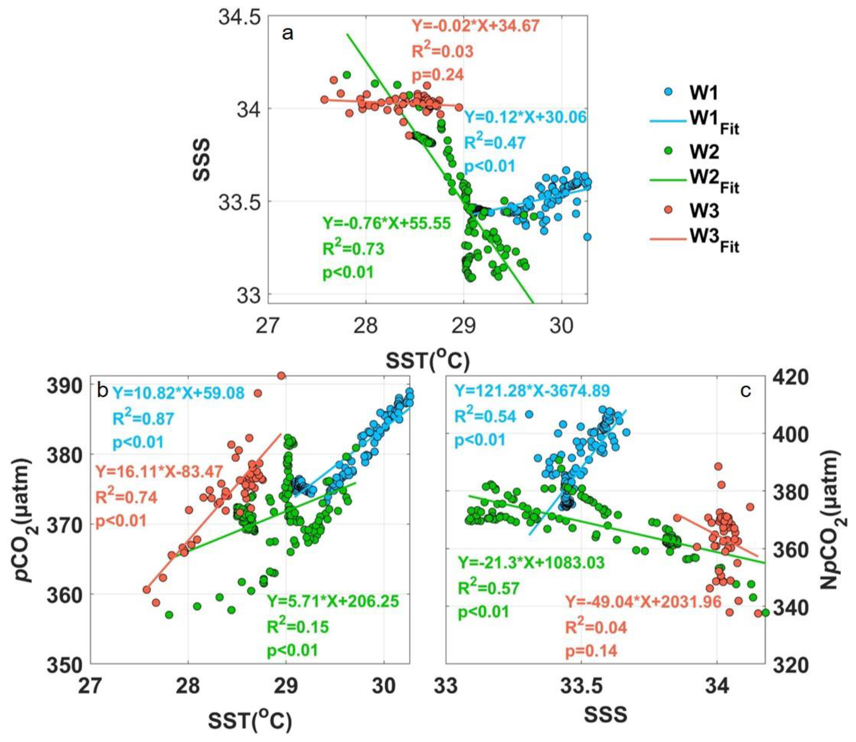
3.1. In Situ Observation of pCO2 and Its Relative Parameters along Transect A

The ship-borne measured data from 3 September to 4 September were used to analyze the variations in SST, SSS, pCO2-sw, pCO2-air, and NpCO2 along Transect A (120°E, 19.5–21.2°N) near the LS (Figure 2). A trough in the curve of pCO2-sw can be found around 20.7–20.9°N along the LS one week after the typhoon (Figure 2b). The distribution of pCO2-sw along Transect A was similar to that of the observed SST and SSS (Figure 2a). The SST reached its minimum value of 27.6 °C at 20.87°N, which was 1.9 °C lower than the average SST value of 19.5–20.4°N (29.5 °C). A maximum SSS of 34.2 psu was located at 20.8°N, indicating an increment of 0.7 psu compared with the average value of 33.5 psu within 19.5–20.4°N (Figure 2a). SSS continued to exhibit higher values between 20.9 and 21.2°N. The average value of pCO2-sw was 380.0 μatm within 19.5–20.4°N, and the lowest value of pCO2-sw (357.0 μatm) occurred at 20.82°N, which was 23.0 μatm lower than the average value of 380.0 μatm (Figure 2b). The pCO2-air was constant at 387.5 μatm (Figure 2b).
To eliminate the influence of temperature, the pCO2-sw was normalized to a reference temperature of 29 °C, which closely approximated the mean SST. The variation in NpCO2 was in the range of 375.1 ± 8.6 μatm along 19.5–21.2°N (Figure 2b).

3.2. Regions Defined by Water Masses from In Situ T-S

The K-means clustering method was employed to classify water masses during the cruise based on temperature–salinity (T-S) profiles. Three different regions of water masses were defined by in situ T-S profiles one week after TC during 3 September to 4 September. Here, the region of each water mass was defined as W1, W2, and W3 respectively. The data of the SCS and KI T-S profile data were drawn according to Chen et al. (1996) [33] and Xu et al. (2018) [34].
W1 with the closest T-S profiles to that of SCS waters, indicating that this region was mainly controlled by SCS waters after TC. W3 was closest to the T-S profiles of Kuroshio waters, indicating that W3 was mainly dominated by KI waters after TC. The T-S characteristics of W2 were situated between those of the SCS water and KI water, indicating that W2 was mainly mixed by the SCS and KI waters after TC (Figure 3).

3.3. Vertical Profile of Isotherm and Currents along Transect A

The deepest MLD (19.7 m) was observed in W1, while the shallowest (7.4 m) was found in W3, with an intermediate MLD (11.0 m) in W2 (Table 2).
A relatively wide range of higher-temperature water was found in the upper 100 m in W1, which indicated downwelling, while an uplift of a 27.5 °C curve in the upper 50 m and downward shift of a 25 °C curve between W2 and W3 were found, which indicated upwelling in shallow water and downwelling in the deeper layers (Figure 4a). The deepest MLD in W1 among three regions (Table 2) was consistent with the downwelling signal found in Figure 4a, while the shallowest MLD in W3 (Table 2) was consistent with the strongest uplift (upwelling) in the center of W3 found in Figure 4a. From the ADCP current data, it can be found that a constantly westward current from the western Pacific Ocean could be found in the northern LS (W3 and to its north), while SCS water constantly traveled eastward to the western Pacific Ocean in the southern LS (W1 and to its south). This proves the accuracy of the processing of the ADCP current data. Combining with these ADCP data, it can be further confirmed that an anticyclone eddy existed in W1 as an anticyclonic current was found in W1, while a cyclonic eddy existed in W3 (westward current in the north and eastward current in the south) and strong fronts (intense flow field variations) existed over the southern part of W2.

3.4. Ekman Pumping Velocity and SST before, during and after Typhoon

The EPVs and wind fields before, during, and after the passage of the TC are depicted in Figure 5. Before TC (21 August), wind blew constantly eastward along the entirety of Transect A (Figure 5a). During the passage of TC (28 August), positive EPVs could be observed almost in all three regions (W1–W3), with the highest EPV appearing in W3, indicating that EPV may induce upwelling in all three regions and the strongest EPV-induced upwelling occur in W3 (Figure 5b). EPVs gradually restored to the pre-TC level one week after the TC (3 September). SST presented a time lag compared with EPV, for which the SST cooling pattern around W2–W3 coincided with the significant positive EPV during the TC and the most significant SST cooling located in W3, where the strongest EPV occurred (Figure 5d–f).

3.5. SLA before, during and after Typhoon

The entirety of W1 and most of W2 were located on the eastern flank of a pre-existing strong anticyclone eddy, while no significant eddy feature was found in W3 one week before the TC (21 August) (Figure 6a). During the TC (28 August), a cyclone eddy generated in the east side near W2 and W3, while W1 was still controlled by an anticyclone eddy (Figure 6b). One week after the TC (3 September), the cyclone eddy strengthened and moved westward into the region where W2 and W3 were located, and W1 started to no longer be controlled by the pre-existing anticyclone eddy (Figure 6c). Combining with those found in the CTD data on the same day after the TC (3 September to 4 September) (Figure 4a), it can be inferred that warmer water subducted in W1 resulted from the warm eddy and the shallow upwelling signal between W2 and W3 resulted from the cold eddy. However, there still remained the question of the downwelling signal between W2 and W3 in a deeper layer (Figure 4a), which will be clarified in the discussion section.

4. Discussion

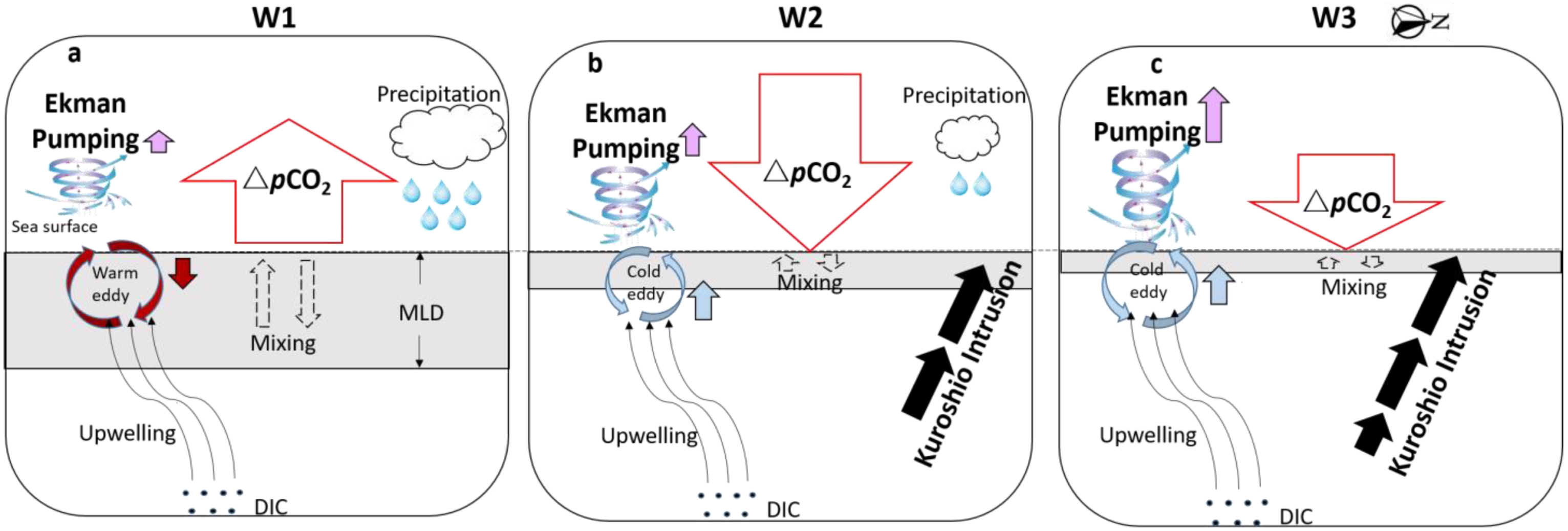
4.1. Effects of Kuroshio Intrusion on pCO2-sw

Compared with the seawater of the SCS, the Kuroshio water was characterized by low surface nutrients, high temperature, and high salinity [18]. Temperature is the primary controlling factor of the pCO2-sw in the SCS [35]. At the same water temperature, the pCO2-sw in the Kuroshio region was lower than that in the SCS [35]. During transportation, the temperature was lowered by radiating heat to the atmosphere, and the pCO2-sw was then reduced through the temperature effect [35]. TCs may also affect the flow direction and intensity of the KI [36].
The variations in the sea surface geostrophic currents (GC) before and after the TC were extracted in this study (Figure 7a–d). The currents of the Kuroshio mainstream (KM) moved northeast along the LS before the TC. TC Nanmadol was at the east side of KM during the early stage of typhoon passage, and it traveled northwestwards into the NESCS and crossed the KM in the middle of LS (Figure 7b). With time, TC Nanmadol gradually modified the trajectory of the KC and bent the KM northeastward following its moving path one and two weeks after the TC (Figure 7c,d), which can be supported by the contour lines of the GC or SLA as well as the KM calculated from each depth of HYCOM data (Figure 7e–i). This conclusion was also supported by the isotherm, where higher temperature and salinity waters appeared deeper than 50 m at 20.8°N (Figure 4a). The flow field with counterclockwise vorticity was also generated during this process one week after the TC, indicating that cyclone eddies can be induced if TCs cause a KI (Figure 7c). Two weeks after the typhoon, the KC shed and its mainstream gradually restored to its pre-TC stage (Figure 7d).
The correlation analysis of temperature, salinity, and pCO2-sw among different regions also revealed interesting findings (Figure 8). The regions influenced by the KC exhibited a negative correlation between temperature and salinity (W2: −0.76; W3: −0.02), and a stronger influence by the KC was associated with a lower significance of the negative correlation (p-value: W2 < 0.01; W3 = 0.24). However, the region dominated by SCS water showed a positive correlation between temperature and salinity (W1: coefficient of 0.12, p-value < 0.01). Additionally, pCO2-sw was jointly governed by temperature and salinity, positively correlated in water dominated by the SCS (W1) (significance coefficients for temperature and salinity), while that in water masses was influenced to a greater extent by the KC (W3 > W2) gradually transitioning from salinity-driven to temperature-driven dynamics (W2: significant correlation between salinity and NpCO2, while temperature and pCO2-sw were less correlated; W3: significant correlation between temperature and pCO2-sw, but no significant correlation with salinity and NpCO2).
Previous research demonstrated a positive correlation between SSS and NpCO2 in the open ocean [16,17], which could also be found in W1 dominated by SCS water (Figure 8c). The significantly different relationship, with a negative correlation, between salinity and NpCO2 in W2 and W3 further proved the accuracy of the water masses clustering. It also revealed that the intrusion of Kuroshio into the SCS might have led to the reversal of the relevance between salinity and NpCO2, and salinity may have dominated the pCO2-sw in the early stage of intrusion, but temperature may have dominated when strong intrusion occurred.

4.2. Wind Pump Effects of Typhoon on pCO2-sw

As the in situ pCO2-sw data in this study were collected after TC Nanmadol, we utilized the monthly averaged values calculated from SOCAT in situ pCO2-sw data around this region (374.9 μatm, which is consistent with previous studies [26,30]) as the pre-TC pCO2-sw. The TC caused strong upper ocean processes due to its slow movement speed (~2.9 m/s) and strong wind speeds when passing through the LS, which could affect pCO2-sw.
After the passage of the TC, the average value of pCO2-sw increased by 5.1 μtam in W1, and decreased by 8.2 μatm and 1.8 μatm in W2–W3, respectively (Figure 9a). The lowest pCO2-sw was 357.0 μatm at 20.8°N (Figure 2a). A trough of pCO2-sw was found at W2–W3. The average pCO2-sw in W3 (373.1 μatm) was 6.9 μatm lower than the average pCO2-sw in W1 (380.0 μatm).
As a result of the TC “Wind Pump” effects, subsurface waters, which were colder and richer in CO2, were uplifted and mixed with the surface water. This dynamic process could lead to a decrease [20,21,22,37,38] or increase [16,17] in pCO2-sw, depending on the dominant influence of cooling or carbon enrichment on carbonate chemistry [39].
In this research, we utilized the EPV, SST, SLA, and rainfall data extracted from satellites to analyze the mechanisms for the changes in pCO2-sw in W1–W3 (Table 3, Figure 9).
The W1 was mainly affected by the SCS waters and less affected by KI due to the characteristics of SST and SSS being similar to that of SCS (Figure 3a). An anti-cyclone eddy was found both pre-TC and post-TC with a positive SLA, even though the decrease in SLA was greater than 0.1 m after TC (Figure 6c and Figure 9f). Meanwhile, the weakest EPV was found in W1 among all three regions, indicating that the weakest EPV-induced SST cooling should be found in W1, rather than in other regions. However, the decrease in SST in W1 was almost the same as that in W3 (where the strongest SST cooling occurred) (Figure 9d). The most vital rainfall in W1, which could induce significant SST cooling and break the upper ocean stratification, may have contributed to the strong SST cooling and upper ocean vertical mixing, where the most substantial MLD deepening with a weakened effect of warm eddy occurred in W1. The most robust vertical mixing after TC may have benefitted the deeper water with high DIC mixing to the surface, which could increase pCO2-sw. Therefore, the TC-induced vigorous vertical mixing was likely the main reason for the increased pCO2-sw in W1 after TC.
The strongest decrease in SLA was found in W2 among the three defined regions, which shifted from a positive SLA to a negative one, demonstrating that a strong cyclone eddy was generated (strongest eddy-induced upwelling among three regions) after TC (Figure 9a–f). A strong EPV (wind-induced upwelling) was also found in this region. The rainfall in W2 was much weaker than that in W1, with slight changes in MLD (indicating insignificant vertical mixing) (Figure 9c). Therefore, the upwelling caused by the EPV and cyclone eddy may dominate the mesoscale upper ocean processes, which would theoretically cause DIC-rich deeper water to uplift to the surface and increase the pCO2-sw. However, pCO2-sw presented a decreasing trend in W2, indicating that other more important processes must dominate pCO2-sw, such as KI (Figure 8).
In W3, a higher increase in EPV was found than that in W2, indicating the strongest EPV-induced upwelling among all three defined regions (Figure 9b–e). Moreover, a more significant negative SLA was found in this region than that in W2, indicating that the strongest cyclone eddy was generated with the strongest eddy-induced upwelling among all three water mass regions (Figure 9f). The larger MLD uplift could also support the above inference (Figure 9c). In theory, these two processes should have caused DIC-rich deeper water mixing to the surface and induce a more significant increase in pCO2-sw than that in W2. However, pCO2-sw also presented a decrease trend similar to that of W2 in this region, indicating that other similar dominant processes must have affected the pCO2-sw in this region, such as stronger KI.
The Argo buoy data also supported the above inference. The salinity and temperature profile data during the passage of the TC were obtained from two Argo floats near Transect A (Figure 10). The locations of selected days of Argo1 data were close to region W1, and those of Argo2 were close to W3 (Figure 1).
Apparent upwelling could be found in Argo1 as a significant uplift of salinity and temperature profiles during the TC in the upper ocean (0–100 m), and upwelling shifted into downwelling in the subsurface layer (20–100 m), which may have been due to continued existence of an anti-cyclone eddy (Figure 10a). All these phenomena were consistent with the above inference in W1 regions.
Upwelling signals could also be found in Argo2 during and after the TC in the shallow surface layer (0–35 m) (Figure 10b), which was consistent with the previous inference in W3 (Figure 7). At the same time, a high salinity and temperature peak could be found around 50 m during TC, and higher salinity and temperature appeared along almost the whole profiles deeper than 50 m during and after the TC, which should be KI, with higher temperature and salinity waters than those of the SCS (Figure 10b). These were also consistent with the above inference that KI was the more important process affecting the pCO2-sw than TC-induced upwelling in W2 and W3.

5. Conclusions

Based on in situ measurements and satellite data, the changes in pCO2-sw following the passage of TC Nanmadol in September 2011 in NESCS were investigated. The physical processes induced by the typhoon “Wind Pump”, including upwelling, vertical mixing, eddy, and KI, were expected to imact the concentration of pCO2-sw. The mechanisms varied in different regions (Figure 11).
(1) In the region dominated by SCS waters (W1), the TC “Wind Pump” induced strong vertical mixing, uplifting DIC-rich deeper water to the surface, and dominated the increase in pCO2-sw after the typhoon.
(2) In the region affected by Kuroshio waters (W2 and W3), pCO2-sw presented a decreasing trend under conditions of TC-enhanced KI with the invasion of lower-pCO2-sw Kuroshio waters.
(3) More significant TC-induced upwelling (EPV-induced upwelling and TC-induced eddy upwelling) would alleviate the decrease in pCO2-sw caused by the TC-enhanced KI.
This research clearly demonstrates the importance of the typhoon “Wind Pump” in changing the air–sea interaction during the passage of typhoons in three different regions. The case presents the source–sink changes in the LS under the influence of a typhoon and also illustrates the non-negligible role of the Kuroshio in estimating carbon fluxes in the SCS. Further analysis and research are needed by combining more measured data for statistical analysis to derive more adequate statistical rules and using model research to clarify the contribution of each process to the carbon cycle.

Author Contributions

Conceptualization, J.L. and D.T.; Data curation, J.L. and Q.S.; Funding acquisition, Y.L. and D.T.; Methodology, J.L. and H.Y.; Visualization, Y.L.; Writing—original draft, J.L.; Writing—review and editing, J.L., Y.L., D.T., X.Z. and Y.G. All authors have read and agreed to the published version of the manuscript.

Funding

This research was funded by Guangdong Special Key Team Program, grant number 2019BT02H594, the Southern Marine Science and Engineering Guangdong Laboratory (Guangzhou), grant number GML2021GD0810, the Major Project of National Social Science Foundation of China, grant number 21ZDA097, the Guangdong Basic and Applied Basic Research Foundation, grant number 2020A1515110196, the Nansha research project, grant number 2022ZD003, the Project of the National Natural Science Foundation of China, grant number 42206186, the Development Fund of South China Sea Institute of Oceanology of the Chinese Academy of Sciences, grant number SCSIO202204, the Independent Research Project Program of State Key Laboratory of Tropical Oceanography, grant number LTOZZ2203, the Key Laboratory of Ocean Space Resource Management Technology, Ministry of Natural Resources, grant number KF-2021-103, and the Key Program of Marine Economy Development Special Foundation of Department of Natural Resources of Guangdong Province, grant numbers GDNRC[2023]41 and GDNRC[2022]20.

Data Availability Statement

Publicly available datasets were analyzed in this study. The typhoon data were obtained from http://weather.unisys.com (accessed on 25 September 2011); the SOCAT data were from https://socat.info/index.php/data-access (accessed on 6 May 2021); the SST data were from http://oceancolor.gsfc.nasa.gov (accessed on 9 December 2020); the wind vectors were from http://manati.star.nesdis.noaa.gov (accessed on 23 June 2022); the SLA datasets were from http://www.aviso.oceanobs.com (accessed on 12 September 2022); the HYCOM data were from http://hycom.org/dataserver/glb-analysis (accessed on 30 September 2022); the rainfall data were from http://www.remss.com (accessed on 26 September 2022); and the Argo float data were from www.argodatamgt.org (accessed on 19 April 2023).

Acknowledgments

We appreciate the South China Sea Open Cruise, R/V Shiyan 3 (SCSIO, CAS) for the in situ data, and also are very thankful to the National Aeronautics and Space Administration (NASA), the Joint Typhoon Warning Center (JTWC), Surface Ocean CO2 Atlas (SOCAT), International Argo Program, Copernicus Marine and Environment Monitoring Service (CMEMS), and the OceanColor Group, National Oceanic and Atmospheric Administration (NOAA), for sharing the datasets.

Conflicts of Interest

The authors declare no conflicts of interest.

References

  1. Takahashi, T.; Sutherland, S.C.; Wanninkhof, R.; Sweeney, C.; Feely, R.A.; Chipman, D.W.; Hales, B.; Friederich, G.; Chavez, F.; Sabine, C. Climatological mean and decadal change in surface ocean pCO2, and net sea–air CO2 flux over the global oceans. Deep Sea Res. Part II Top. Stud. Oceanogr. 2009, 56, 554–577. [Google Scholar] [CrossRef]
  2. Takahashi, T.; Sutherland, S.C.; Sweeney, C.; Poisson, A.; Metzl, N.; Tilbrook, B.; Bates, N.; Wanninkhof, R.; Feely, R.A.; Sabine, C. Global sea–air CO2 flux based on climatological surface ocean pCO2, and seasonal biological and temperature effects. Deep Sea Res. Part II Top. Stud. Oceanogr. 2002, 49, 1601–1622. [Google Scholar] [CrossRef]
  3. Lévy, M.; Lengaigne, M.; Bopp, L.; Vincent, E.M.; Madec, G.; Ethé, C.; Kumar, D.; Sarma, V.V.S.S. Contribution of tropical cyclones to the air-sea CO2 flux: A global view. Glob. Biogeochem. Cycles 2012, 26, GB2001. [Google Scholar] [CrossRef]
  4. Dai, M.H.; Meng, F.F. Carbon cycle in the South China Sea: Flux, controls and global implications. Sci. Technol. Rev. 2020, 38, 30–34. (In Chinese) [Google Scholar] [CrossRef]
  5. Zhai, W.; Dai, M.; Cai, W.-J.; Wang, Y.; Hong, H. The partial pressure of carbon dioxide and air–sea fluxes in the northern South China Sea in spring, summer and autumn. Mar. Chem. 2005, 96, 87–97. [Google Scholar] [CrossRef]
  6. Tseng, C.M.; Wong, G.T.F.; Chou, W.C.; Lee, B.S.; Sheu, D.D.; Liu, K.K. Temporal variations in the carbonate system in the upper layer at the SEATS station. Deep Sea Res. Part II Top. Stud. Oceanogr. 2007, 54, 1448–1468. [Google Scholar] [CrossRef]
  7. Dai, M.; Cao, Z.; Guo, X.; Zhai, W.; Liu, Z.; Yin, Z.; Xu, Y.; Gan, J.; Hu, J.; Du, C. Why are some marginal seas sources of atmospheric CO2? Geophys. Res. Lett. 2013, 40, 2154–2158. [Google Scholar] [CrossRef]
  8. Li, Q.; Guo, X.; Zhai, W.; Xu, Y.; Dai, M. Partial pressure of CO2 and air-sea CO2 fluxes in the South China Sea: Synthesis of an 18-year dataset. Prog. Oceanogr. 2020, 182, 102272. [Google Scholar] [CrossRef]
  9. Chern, C.-S.; Wang, J. A numerical study of the summertime flow around the Luzon Strait. J. Oceanogr. 1998, 54, 53–64. [Google Scholar] [CrossRef]
  10. Sui, Y.; Sheng, J.; Tang, D.; Xing, J. Study of storm-induced changes in circulation and temperature over the northern South China Sea during Typhoon Linfa. Cont. Shelf Res. 2022, 249, 104866. [Google Scholar] [CrossRef]
  11. Zhang, H.; He, H.; Zhang, W.-Z.; Tian, D. Upper ocean response to tropical cyclones: A review. Geosci. Lett. 2021, 8, 1. [Google Scholar] [CrossRef]
  12. Liu, Y.; Tang, D.; Evgeny, M. Chlorophyll Concentration Response to the Typhoon Wind-Pump Induced Upper Ocean Processes Considering Air–Sea Heat Exchange. Remote Sens. 2019, 11, 1825. [Google Scholar] [CrossRef]
  13. Ye, H.; Tang, S.; Morozov, E. Variability in Sea Surface pCO2 and Controlling Factors in the Bay of Bengal Based on buoy Observations at 15°N, 90°E. J. Geophys. Res. Ocean. 2022, 127, e2022JC018477. [Google Scholar] [CrossRef]
  14. Ye, H.; Sheng, J.; Tang, D.; Morozov, E.; Kalhoro, M.A.; Wang, S.; Xu, H. Examining the Impact of Tropical Cyclones on Air-Sea CO2 Exchanges in the Bay of Bengal Based on Satellite Data and In Situ Observations. J. Geophys. Res. Ocean. 2019, 124, 555–576. [Google Scholar] [CrossRef]
  15. Sun, Q.; Lin, J.; Tang, D.; Pan, G.; Jiang, Z. Different mechanisms of air-sea CO2 exchange respond to “Wind Pump” effect of two tropical cyclones. Ecol. Sci. 2020, 39, 9–16. (In Chinese) [Google Scholar] [CrossRef]
  16. Sun, Q.; Tang, D.; Legendre, L.; Shi, P. Enhanced sea-air CO2 exchange influenced by a tropical depression in the South China Sea. J. Geophys. Res. Ocean. 2014, 119, 6792–6804. [Google Scholar] [CrossRef]
  17. Ye, H.; Sheng, J.; Tang, D.; Siswanto, E.; Ali Kalhoro, M.; Sui, Y. Storm-induced changes in pCO2 at the sea surface over the northern South China Sea during Typhoon Wutip. J. Geophys. Res. Ocean. 2017, 122, 4761–4778. [Google Scholar] [CrossRef]
  18. Liu, Y.; Tang, D.; Tang, S.; Morozov, E.; Liang, W.; Sui, Y. A case study of Chlorophyll a response to tropical cyclone Wind Pump considering Kuroshio invasion and air-sea heat exchange. Sci. Total Environ. 2020, 741, 140290. [Google Scholar] [CrossRef]
  19. Lin, J.; Tang, D.; Alpers, W.; Wang, S. Response of dissolved oxygen and related marine ecological parameters to a tropical cyclone in the South China Sea. Adv. Space Res. 2014, 53, 1081–1091. [Google Scholar] [CrossRef]
  20. Nemoto, K.; Midorikawa, T.; Wada, A.; Ogawa, K.; Takatani, S.; Kimoto, H.; Ishii, M.; Inoue, H.Y. Continuous observations of atmospheric and oceanic CO2 using a moored buoy in the East China Sea: Variations during the passage of typhoons. Deep Sea Res. Part II Top. Stud. Oceanogr. 2009, 56, 542–553. [Google Scholar] [CrossRef]
  21. Yu, P.; Wang, Z.A.; Churchill, J.; Zheng, M.; Pan, J.; Bai, Y.; Liang, C. Effects of Typhoons on Surface Seawater pCO2 and Air-Sea CO2 Fluxes in the Northern South China Sea. J. Geophys. Res. Ocean. 2020, 125, e2020JC016258. [Google Scholar] [CrossRef]
  22. Kao, K.J.; Huang, W.J.; Chou, W.C.; Gong, G.C.; Weerathunga, V. Factors Controlling the Sea Surface Partial Pressure of Carbon Dioxide in Upwelling Regions: A Case Study of the Southern East China Sea Before and after Typhoon Maria. J. Geophys. Res. Ocean. 2023, 128, e2022JC019195. [Google Scholar] [CrossRef]
  23. Shih, Y.-Y.; Hung, C.-C.; Huang, S.-Y.; Muller, F.L.; Chen, Y.-H. Biogeochemical variability of the upper ocean response to typhoons and storms in the northern South China Sea. Front. Mar. Sci. 2020, 7, 151. [Google Scholar] [CrossRef]
  24. Ning, J.; Xu, Q.; Zhang, H.; Wang, T.; Fan, K. Impact of cyclonic ocean eddies on upper ocean thermodynamic response to typhoon Soudelor. Remote Sens. 2019, 11, 938. [Google Scholar] [CrossRef]
  25. Tsao, S.-E.; Shen, P.-Y.; Tseng, C.-M. Rapid increase of pCO2 and seawater acidification along Kuroshio at the east edge of the East China Sea. Mar. Pollut. Bull. 2023, 186, 114471. [Google Scholar] [CrossRef] [PubMed]
  26. Zhai, W. Sea Surface partial pressure of CO2 and its controls in the northern South China Sea in the non bloom period in spring. Haiyang Xuebao 2015, 37, 31–40. (In Chinese) [Google Scholar] [CrossRef]
  27. Chou, W.C.; Sheu, D.D.; Chen, C.A.; Wen, L.S.; Yang, Y.; Wei, C.L. Transport of the South China Sea subsurface water outflow and its influence on carbon chemistry of Kuroshio waters off southeastern Taiwan. J. Geophys. Res. Ocean. 2007, 112, C12008. [Google Scholar] [CrossRef]
  28. Li, C.; Zhai, W.; Qi, D. Unveiling controls of the latitudinal gradient of surface pCO2 in the Kuroshio Extension and its recirculation regions (northwestern North Pacific) in late spring. Acta Oceanol. Sin. 2022, 41, 110–123. [Google Scholar] [CrossRef]
  29. Fan, L.-F.; Chow, C.H.; Gong, G.-C.; Chou, W.-C. Surface Seawater pCO2 Variation after a Typhoon Passage in the Kuroshio off Eastern Taiwan. Water 2022, 14, 1326. [Google Scholar] [CrossRef]
  30. Zhai, W.D.; Dai, M.H.; Chen, B.S.; Guo, X.H.; Li, Q.; Shang, S.L.; Zhang, C.Y.; Cai, W.J.; Wang, D.X. Seasonal variations of sea–air CO2 fluxes in the largest tropical marginal sea (South China Sea) based on multiple-year underway measurements. Biogeosciences 2013, 10, 7775–7791. [Google Scholar] [CrossRef]
  31. Price, J.F. Upper ocean response to a hurricane. J. Phys. Oceanogr. 1981, 11, 153–175. [Google Scholar] [CrossRef]
  32. Obata, A.; Ishizaka, J.; Endoh, M. Global verification of critical depth theory for phytoplankton bloom with climatological in situ temperature and satellite ocean color data. J. Geophys. Res. Ocean. 1996, 101, 20657–20667. [Google Scholar] [CrossRef]
  33. Chen, C.T.A.; Huang, M.H. A mid-depth front separating the South China Sea water and the Philippine sea water. J. Oceanogr. 1996, 52, 17–25. [Google Scholar] [CrossRef]
  34. Xu, W.L.; Wang, G.F.; Zhou, W.; Xu, Z.T.; Cao, W.X. Vertical variability of chlorophyll a concentration and its responses to hydrodynamic processes in the northeastern South China Sea in summer. J. Trop. Oceanogr. 2018, 37, 62–73. (In Chinese) [Google Scholar] [CrossRef]
  35. Zhai, W.; Dai, M.; Cai, W.-J.; Wang, Y.; Wang, Z. High partial pressure of CO2 and its maintaining mechanism in a subtropical estuary: The Pearl River estuary, China. Mar. Chem. 2005, 93, 21–32. [Google Scholar] [CrossRef]
  36. Guo, L.; Xiu, P.; Chai, F.; Xue, H.; Wang, D.; Sun, J. Enhanced chlorophyll concentrations induced by Kuroshio intrusion fronts in the northern South China Sea. Geophys. Res. Lett. 2017, 44, 11565–11572. [Google Scholar] [CrossRef]
  37. Bates, N.R.; Knap, A.H.; Michaels, A.F. Contribution of hurricanes to local and global estimates of air–sea exchange of CO2. Nature 1998, 395, 58–61. [Google Scholar] [CrossRef]
  38. Huang, P.; Imberger, J. Variation of pCO2 in ocean surface water in response to the passage of a hurricane. J. Geophys. Res. Ocean. 2010, 115, C10024. [Google Scholar] [CrossRef]
  39. Ye, H.; Morozov, E.; Tang, D.; Wang, S.; Liu, Y.; Li, Y.; Tang, S. Variation of pCO2 concentrations induced by tropical cyclones “Wind-Pump” in the middle-latitude surface oceans: A comparative study. PLoS ONE 2020, 15, e0226189. [Google Scholar] [CrossRef]
Figure 1. The track of tropical cyclone (TC) Nanmadol and the positions of five in situ stations (S1–S5) on Transect A (120°E, 19.5°N to 21.5°N). The TC centers are denoted by circles with colors indicating TC wind speed. The in situ stations are denoted by black triangles. The tracks of Argo floats are denoted by squares (Argo1: 1 August to 6 September, Argo2: 8 August to 7 September), and the five-pointed star indicates the starting point of the Argo.
Remotesensing 16 00123 g001
Figure 2. Variations in SST, SSS, pCO2-sw, pCO2-air, and NpCO2 along Transect A from 3 September to 4 September in 2011. (a) SST (orange) and SSS (navy blue), (b) pCO2-sw (green), NpCO2 (pink), and pCO2-air (purple dash). Org indicates the original points.
Remotesensing 16 00123 g002
Figure 3. Water mass clustered using K-means along Transect A over the LS. (a) T-S diagram of the in situ data along Transect A and climatological SCS and KI waters. (b) Horizontal distribution of the three regions defined by water masses clustering results. W1: blue, W2: yellow, W3: orange.
Remotesensing 16 00123 g003
Figure 4. Vertical profiles of temperature and acoustic Doppler current profiler (ADCP) currents. (a) Isotherms derived from CTD. (b) ADCP currents. The blue dashed line indicates the isotherm of 27.5 °C. The distribution of the currents was measured at depths ranging from 38 to 294 m, with an interval of 16 m between each depth level. The black dashed lines identify the horizontal distributions of the three defined regions.
Remotesensing 16 00123 g004
Figure 5. Ekman pumping velocity (EPV) and SST before, during, and after the passage of the TC. Arrows indicate wind fields. The three colored lines (blue, yellow, and red) indicate the three defined regions (W1–W3), respectively. (ac) indicate EPV one week before, during, and one week after the TC, respectively. (df) indicate the SST one week before, during, and one week after the TC, respectively.
Remotesensing 16 00123 g005
Figure 6. Sea level anomaly (SLA) before, during, and after the TC. (a) SLA one week before the TC, (b) SLA during the TC, and (c) SLA one week after the TC. The black dots and lines indicate the typhoon path. The three colored lines indicate the three defined regions.
Remotesensing 16 00123 g006
Figure 7. Geostrophic currents (GC) and Kuroshio mainstream (KM) extracted by the HYCOM model flow field changes before, during, and after the TC. (a) GC one week before the TC, (b) GC during the TC, (c) GC one week after the TC, (d) GC two weeks after the TC, (e) KM at 75 m depth, (f) KM at 100 m depth, (g) KM at 125 m depth, (h) KM at 150 m depth, and (i) KM at 200 m depth. The colored lines indicate the three defined regions. The red boxes indicate the location of the Kuroshio intrusion.
Remotesensing 16 00123 g007
Figure 8. The correlations between different oceanographic variables of the three defined regions along Transect A from 3 September to 4 September in 2011. (a) SST and SSS, (b) SST and pCO2-sw, and (c) SSS and NpCO2.
Remotesensing 16 00123 g008
Figure 9. The comparison of pCO2-sw and other environmental parameters before and after the typhoon in the three defined regions. (a) pCO2-sw, (b) EPV, (c) MLD, (d) SST, (e) Rainfall, (f) SLA, and (g) the normalized difference of the parameters.
Remotesensing 16 00123 g009
Figure 10. The vertical distributions of salinity (black) and temperature (red) from the surface to 300 m depths before, during, and after the TC from Argo1 and Argo2. (a) Argo1; (b) Argo2. The full line curve indicates pre-TC, the dashed line curve indicates during TC, and the dotted line curve indicates post-TC.
Remotesensing 16 00123 g010
Figure 11. Schematic diagram of the three influencing mechanisms in the three defined regions caused by both the typhoon “Wind Pump” and Kuroshio Intrusion (KI). (a) Influencing mechanism in W1 (TC rain-induced vertical mixing), (b) influencing mechanism in W2 (KI and TC-induced upwelling), and (c) influencing mechanism in W3 (TC-enhanced KI and TC-induced stronger upwelling). The red unfilled up/down arrows indicate the increment/decline of pCO2-sw after the typhoon. The black filled arrows indicate the Kuroshio intrusion. The red filled anti-cyclonic arrows indicate the warm eddy, while the blue filled cyclonic arrows indicate the cold eddy. The gray box indicates the MLD. The purple filled arrows indicate Ekman Pumping. The red/blue filled arrows indicate the weaken/strengthen in the eddy. The shape and size of the signals indicate the magnitude of the variables.
Remotesensing 16 00123 g011
Table 1. Lists of data used in this research.
Order NumberData TypeData NameInformation
1Typhoon trackTyphoon track6-hourly time series
2In situ datapCO2-swVessel-mounted; 70 s/record, and averaged every 3 min
3SOCAT pCO2Jan 2008 to April 2009
4SSTEvery in situ station; 5 s/record, and averaged every 3 min
5SSSEvery in situ station; 5 s/record, and averaged every 3 min
6ADCP currentEvery in situ station; 16 m per interval
7Argo floats5–200 m depths
8Satellite and model dataWind fieldSpatial resolution: 25 km; daily
9SSTSpatial resolution: 4 km × 4 km; Temporal resolution: 8 days
10SLASpatial resolution: 1/3° × 1/3°; Temporal resolution: 7 days
11PrecipitationSpatial resolution: 0.25° × 0.25°; Temporal resolution: 7 days
12HYCOM1/12° equatorial resolution
Table 2. Statistics of MLD, SST, SSS, pCO2-sw, NpCO2, and pCO2-air of the three defined regions (W1–W3) in Transect A from 3 September to 4 September in 2011.
RegionData Collecting TimeLocation (°N)Sample QuantityMLD
(m)
SST (°C)SSS (psu)pCO2-sw
(μatm)
NpCO2
(μatm)
pCO2-air
(μatm)
W14 September 201119.49–20.3616119.729.5 ± 0.433.5 ± 0.1378.7 ± 4.6386.6 ± 11.0387.5
W24 September 201120.37–20.8213611.028.9 ± 0.3333.6 ± 0.3371.2 ± 4.91368.7 ± 8.3387.5
W33 September 201120.83–21.20587.428.43 ± 0.3134.0 ± 0.1374.3 ± 6.0364.3 ± 10.3387.5
Table 3. Summary of the normalized difference in pCO2-swpCO2-sw), EPV (ΔEPV), mixed layer depth (ΔMLD), SST (ΔSST), rainfall (ΔRainfall), and SLA (ΔSLA) before and after the passage of the TC in the three defined regions (W1–W3).
Water MassΔpCO2-swΔEPVΔMLDΔSSTΔRainfallΔSLA
W10.620.241−0.971−0.68
W2−10.74−0.24−0.990.63−1
W3−0.221−0.28−10.03−0.91
Disclaimer/Publisher’s Note: The statements, opinions and data contained in all publications are solely those of the individual author(s) and contributor(s) and not of MDPI and/or the editor(s). MDPI and/or the editor(s) disclaim responsibility for any injury to people or property resulting from any ideas, methods, instructions or products referred to in the content.

