A Reference-Free Method for the Thematic Accuracy Estimation of Global Land Cover Products Based on the Triple Collocation Approach

Abstract

Global land cover (GLC) data are an indispensable resource for understanding the relationship between human activities and the natural environment. Estimating their classification accuracy is significant for studying environmental change and sustainable development. With the rapid emergence of various GLC products, the lack of high-quality reference data poses a severe risk to traditional accuracy estimation methods, in which reference data are always required. Thus, meeting the needs of large-scale, fast evaluation for GLC products becomes challenging. The triple collocation approach (TCCA) is originally applied to assess classification accuracy in earthquake damage mapping when ground truth is unavailable. TCCA can provide unbiased accuracy estimation of three classification systems when their errors are conditionally independent. In this study, we extend the idea of TCCA and test its performance in the accuracy estimation of GLC data without ground reference data. Firstly, to generate two additional classification systems besides the original GLC data, a k-order neighbourhood is defined for each assessment unit (i.e., geographic tiles), and a local classification strategy is implemented to train two classifiers based on local samples and features from remote sensing images. Secondly, to reduce the uncertainty from complex classification schemes, the multi-class problem in GLC is transformed into multiple binary-class problems when estimating the accuracy of each land class. Building upon over 15 million sample points with remote sensing features retrieved from Google Earth Engine, we demonstrate the performance of our method on WorldCover 2020, and the experiment shows that screening reliable sample points during training local classifiers can significantly improve the overall estimation with a relative error of less than 4% at the continent level. This study proves the feasibility of estimating GLC accuracy using the existing land information and remote sensing data, reducing the demand for costly reference data in GLC assessment and enriching the assessment approaches for large-scale land cover data.

1. Introduction

Since the Global Land Cover Characterisation dataset was first released in the early 1990s, tremendous efforts have been made to produce global land cover (GLC) products towards better accuracy and resolution [1,2]. Benefiting from remote sensing and artificial intelligence techniques, GLC production efficiency has significantly improved in the last decades. More than 10 GLC products with up to 10 m resolution are available now [3,4,5,6,7]. These GLC products provide unprecedented details of the Earth’s surface and promote a batch of studies on environmental, biological and social sciences on a global scale [8,9,10,11].

The application scope of a GLC product is significantly affected by its uncertainty, which many factors can influence, including the definition of the classification scheme (e.g., the hierarchy and description of land classes) [12], mapping scale (e.g., the minimum mapping unit) [13], input data (e.g., satellite image) and classification methods [14]. Thematic accuracy assessment is a fundamental procedure for producers and users to learn the uncertainty in GLC data and thus make rational decisions [12,15]. Currently, most GLC datasets are assessed by comparison with ground reference data. The confusion matrix, together with some related descriptive metrics such as the overall accuracy (OA), user accuracy (UA) and producer accuracy (PA), is used to characterise the accuracy [5,16,17]. Reference data are commonly collected based on a stratified random sampling design, in which the true class for each sample point is determined by either field survey or visual interpretation using high-resolution satellite images [15,18]. However, given the huge amount of sample points needed for GLC assessment, obtaining sufficient high-quality reference data on a global scale is always laborious and time-consuming [19,20,21].

Considerable efforts have been made to reduce the cost of reference data collection, such as utilising open data sources such as OpenStreetMap or establishing web-based platforms to collect crowdsourcing data from global volunteers for the validation of specific GLC products [22,23,24,25]. A recent example can be seen in the validation of GlobeLand30, in which an online system GLCVal was designed and used by approximately 30 countries and international organisations for collaborative assessment [26]. Crowdsourcing also indicates a promising direction for GLC assessment with the increasing popularity of geotagged social media and related mobile apps [27,28]. However, significant concerns are raised about the reliability of crowdsourcing data because of the varying expertise of volunteers, and the uneven distribution of volunteers would possibly lead to very few sample points in some regions [29,30].

Considering the limitation of sample-based assessment, some scientists seek to estimate accuracy without standard reference data. Given the availability of vast global and regional land cover products, various cross-comparison strategies were proposed to investigate the spatial, semantic or areal consistency between different GLC datasets [31,32,33]. The conversion of GLC products with heterogeneous classification systems is the first step to enabling cross-comparison [34]. Considerable efforts have been made to harmonise different land cover products, for example, by converting them into a standard classification system or developing fuzzy approaches based on the semantic similarity in the definition of land classes [32,33]. However, these methods require many subjective rules and present several difficulties in dealing with complex land classes, which makes the conversion of various GLC products still a challenging practice [35,36,37].

Instead of rigorous accuracy estimation, some studies have attempted to identify potentially erroneous land objects without reference data, in which models based on outlier detection techniques were widely adopted. A typical example can be seen in Radoux and Defourny (2010) [38], where probabilistic outliers in terms of spectral features were detected based on an iterative trimming method. This method was also extended to extract reliable samples for GLC mapping [39]. To overcome the possible failure of statistical assumptions in detecting outlying land objects, Chen et al. developed a series of reference-free methods by adopting proximity-based outlier detection techniques and proposed several quantitative measures of the reliability of land cover vector data [40] and raster data [21]. Although these methods are useful as an auxiliary tool to assist the manual inspection and the improvement of land cover products, they cannot estimate the confusion matrix and fail to provide explicit information of accuracy.

Another batch of model-based studies took the ground truth as an unobserved (latent) variable. Inference models, such as the latent class model (LCM) and triple collocation approach (TCCA (The acronym TCCA is used following the original study of Pierdicca et al. [41])), were adapted to estimate the thematic accuracy based on additional labels for each land case [13,41,42,43,44]. Specially, TCCA was established to estimate the confusion matrixes of three classification systems without reference data. The estimation was proven unbiased when the three systems’ errors were conditionally independent [41]. These pioneering works verified the feasibility of estimating land cover accuracy without ground reference data, and TCCA seems promising because it can provide rich accuracy information (e.g., the confusion matrix) rather than a single accuracy metric. However, a critical issue emerges when applying TCCA to the assessment of GLC. Given that a GLC product could be deemed as a single snapshot of the surface at a specific point in time, no other independent versions of GLC follow the same classification scheme and specification that can directly serve as the additional two systems to build up the foundation of TCCA. Furthermore, given the massive data and unbalanced distribution of GLC, the performance of TCCA in GLC accuracy estimation remains unclear.

This study aims to investigate strategies for using TCCA when only a single classification dataset is available and, thus, proposes a feasible workflow for estimating GLC accuracy without reference data. To reduce the influence of complex classification schemes, the multi-class problem in GLC is transformed into multiple binary-class problems when estimating the accuracy of each land class. Taking geographic tiles as the basic assessed unit, two local classifiers are independently trained for each land class of each assessed tile based on samples randomly selected from its neighbouring tiles. To ensure the basic assumption on conditional independence of TCCA, a Gaussian density function is applied to weight the number of samples from neighbouring tiles of different orders. These local classifiers are then applied to predict the land labels of the assessed unit, and the resultant local classifications and the original one are taken as the input of TCCA to estimate the classification accuracy. We also explore the effectiveness of the outlier detection technique in extracting reliable local samples, which might reduce errors in local classifications that are inherited from the original data and thus avoid the potential violation of conditional independence. Building upon over 15 million sample points retrieved from Google Earth Engine (GEE) and model parameters tuned from a regional land cover dataset, LandCover-Net Africa (LCN-AFR), we test the performance of our approach on high-resolution GLC datasets, European Space Agency (ESA) WorldCover 2020. Our approach is expected to provide a low-cost solution for a rapid investigation of the spatial accuracy of GLC and enrich the methodological framework of GLC mapping.

2. Methods

2.1. Mathematical Foundation of TCCA

The triple collocation technique was initially developed for modelling the errors in ocean wind speed retrievals [45] and subsequently adopted in the assessment of many geophysical variables, such as soil moisture [46], sea surface salinity [47] and precipitation [48]. Concerning discrete variables in classification problems, Pierdicca et al. [41] conceived the TCCA model to estimate the confusion matrixes of three classification systems without ground truth data.

Let $X,Y \mathrm{and} Z$ denote the three systems, and $\Theta$ be the unobserved ground truth. The sample points associated with each $X,Y,Z$ system and $\Theta$ are denoted as $x,y,z$ and $\theta$, respectively. The basic assumption of TCCA is that the errors of $X,Y,Z$ are conditionally independent (e.g., $P\left(x|y,\theta \right)=P\left(x,\theta \right)$), and thus the following equation is obtained:

$$P(x,y,\theta )=P(x|y,\theta )P(y,\theta )=\frac{P(x,\theta )P(y,\theta )}{P(\theta )}$$

(1)

By marginalising over parameter $\theta$, we could obtain the joint probability $P\left(x,y\right)$, which is equivalent to the confusion matrix of $X,Y$ systems. The element of the confusion matrix XY can be expressed as follows:

$$p_{i,j}^{XY}={\displaystyle \sum _{k=1}^N\frac{p_{i,k}^{X\mathsf{\Theta }}{p}_{i,k}^{Y\mathsf{\Theta }}}{p_k^{\mathsf{\Theta }}}}$$

(2)

where $p_{i,k}^{X\mathsf{\Theta }}$ denotes the joint probability for a sample point of a true class $k$ being labelled as class $i$ in system $X$, and $p_k^{\mathsf{\Theta }}$ is the probability for a sample point belonging to class $k$ in ground truth $\mathsf{\Theta }$.

According to Equation (2), the target confusion matrixes $X\mathsf{\Theta }$, $Y\mathsf{\Theta }$ and $Z\mathsf{\Theta }$ in accuracy estimation should satisfy the following equations after some matrix operations:

$$\begin{array}{l}X\mathsf{\Theta }\cdot P\cdot X{\mathsf{\Theta }}^T=XZ\cdot Y{Z}^{-1}\cdot X{Y}^T\\ Y\mathsf{\Theta }\cdot P\cdot Y{\mathsf{\Theta }}^T=YZ\cdot X{Z}^{-1}\cdot XY\\ Z\mathsf{\Theta }\cdot P\cdot Z{\mathsf{\Theta }}^T=Y{Z}^T\cdot X{Y}^{-1}\cdot XZ\end{array}$$

(3)

where P is a diagonal matrix composed of $\frac{1}{p_k^{\mathsf{\Theta }}}$ ($k=1,\dots ,N$). Additionally, considering the prevalence of each class in $\mathsf{\Theta }$, one can obtain the following constraints:

$$p_k^{\mathsf{\Theta }}={\displaystyle \sum _{i=1}^N{p}_{i,j}^{X\mathsf{\Theta }}}={\displaystyle \sum _{i=1}^N{p}_{i,j}^{Y\mathsf{\Theta }}}={\displaystyle \sum _{i=1}^N{p}_{i,j}^{Z\mathsf{\Theta }}}$$

(4)

Considering the joint probability $P\left(x,y,z,\theta \right)$ similar to the deduction in Equations (1) and (2), one can obtain additional constraints:

$$p_{i,j,k}^{X,Y,Z}={\displaystyle \sum _{m=1}^N\frac{p_{i,m}^{X,\mathsf{\Theta }}{p}_{j,m}^{Y,\mathsf{\Theta }}{p}_{k,m}^{Z,\mathsf{\Theta }}}{{(p_m^{\mathsf{\Theta }})}^2}}$$

(5)

Finally, together with Equations (3)–(5), the target confusion matrixes $X\mathsf{\Theta }$, $Y\mathsf{\Theta }$ and $Z\mathsf{\Theta }$ can be obtained with some algebraic operations, and more computational details can be found in the original paper [41].

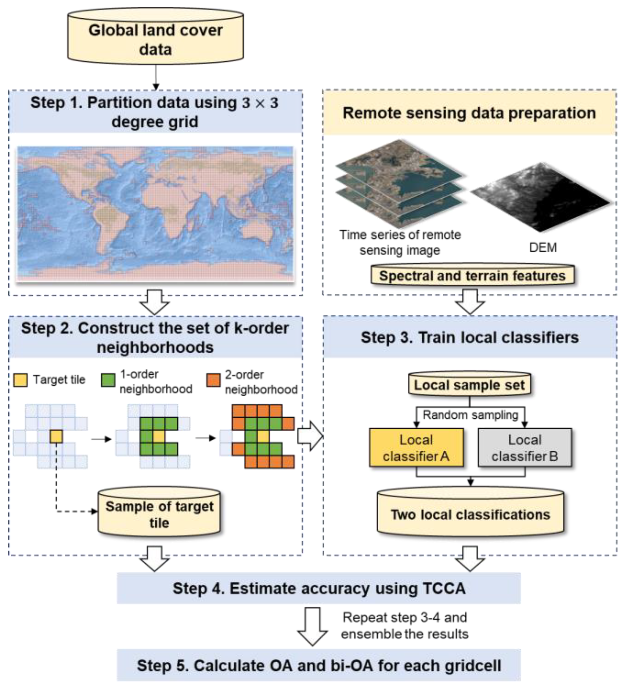
2.2. Solution for TCCA Applied to GLC Assessment

To distinguish our method from the original TCCA, we termed our method GLC-TCCA in the following contents. The workflow of GLC-TCCA is shown in Figure 1. The core of GLC-TCCA is to generate additional two classification system based on local classifiers trained by samples from neighbouring tiles of the assessed one. Indeed, training local classifiers is not unusual in current land cover production [39,49,50]. Given the heterogeneity of the surface, a local classifier is expected to achieve better classification accuracy than a global one by adaptively learning the regional characteristics of the land. Sample for training local classifiers are obtained by either manual interpretation or derived from the existing land cover products [51]. While manual interpretation generally provides reliable samples but involves a huge workload [52], deriving samples from existing datasets has been demonstrated to be much more efficient and allows the resultant classifications to follow the same classification scheme, making it increasingly popular in large-scale land cover mapping [51,53]. The processes will be introduced step by step in the following subsections.

2.2.1. Data Partition

The GLC dataset is first partitioned using specific geographical tiles (e.g., a 3 × 3 degree grid). This step aims to determine the assessed unit in the estimation and reduce the data size processed at once.

2.2.2. Neighbourhood Construction

Training sample points are randomly selected from the training pool of each tile $t$, which is here defined as its neighbourhood set ${\mathsf{\Phi }}_k\left(t\right)=\left\{{\varphi }_1,\dots ,{\varphi }_k\right\}$, where ${\varphi }_i$ is the i-order neighbourhood of $t_i$ as shown in Figure 1, and $k$ is the maximum order considered here. Unlike the common definition of the neighbourhood as the adjacent 3 × 3 tiles [51,54], the adoption of a high-order neighbourhood would introduce a certain amount of sample points from distant tiles into the training phase. According to Tobler’s First Law of Geography [55], points that are distant from $t$ would be less related to the ones from t. Given the basic assumption of TCCA, that is, the errors of the three systems should be conditionally independent to generate unbiased estimation [41], using a high-order neighbourhood set is expected to increase further the independence between ${\mathsf{\Phi }}_k\left(t\right)$ and $t$, while keeping the effectiveness of local classifiers as local features are still captured. However, as high-order neighbourhoods would dominate ${\mathsf{\Phi }}_k\left(t\right)$ with an increase in k, this study adopts a Gaussian density function to determine the number of sample points $m_i$ from the i-order neighbourhood, which can be written as:

$$m_i=M\times \frac{\mathrm{Norm}(u,{\sigma }^2)}{{\displaystyle \sum _{i=1}^k\mathrm{Norm}(u,{\sigma }^2)}}$$

(6)

where the $\mathrm{Norm}\left(u,{\sigma }^2\right)$ refers to the Gaussian density function with the expectation of $u$ and standard deviation of $\mathsf{\sigma }$. $M$ is the total number of sample points for training. For simplicity, $\sigma$ is set to 1, and $k$ is set to 9 in this study, while the optimal value of $u$ is tuned by the simulation experiment discussed in Section 3.2.

2.2.3. Training Two Local Classifiers

By taking the sample points’ class label as the dependent variable, two different classifiers were trained on a balanced dataset using features from remote sensing data. To reduce the correlation between the two local classification systems, the classifiers were trained using exclusive points. It should be notable that since the two classifiers have different mechanisms and are trained on different bases, their errors tend to be uncorrelated [44,56].

The local classifiers were subsequently applied to $t_i$ so that two additional systems could be obtained for further analysis using TCCA. Given the widely existing spatial heterogeneity in large-scale land cover data [57,58], the classification errors in different tiles are also likely to present different distributions. In this regard, the correlation between the original classification and the one predicted by local classifier could be largely reduced using the sample from the defined neighbourhood in this study.

Finally, to increase the robustness of our method, the training and analysis phases were repeated multiple times with different random samples, and the results were combined to obtain the final estimation of the thematic accuracy.

2.2.4. Estimating the Accuracy for a Single Class

TCCA is theoretically capable of handling multi-class problems with the complexity of approximately $\mathrm{O}\left(n^2\right)$, which would significantly increase with a larger number of classes [41]. Therefore, in this study, considering various classification schemes in GLC projects, we transform the multi-class problem into multiple binary-class problems by iteratively taking one class as positive and the rest as negative. This operation has at least two advantages. Firstly, the model uncertainty from local classifiers and TCCA would be vastly reduced as the number of classes decreases [59]. Secondly, the sample space, which determines the possible outcome of an experiment, will significantly change as some classes are merged [60]. As a result, the correctness of the reformed dichotomous data would be theoretically higher than the raw one, which might help to reduce the potential error correlation between the local classification systems and the original one to improve the effectiveness of TCCA.

2.2.5. Estimating the Overall Accuracy

One issue raised by the transformation mentioned above is the ensembling of accuracy metrics: one can only obtain the accuracy estimation for a single class for each binary-class case, while the accuracy information (e.g., the OA) of the entire data is not directly measured. The present study takes OA as an example to demonstrate the calculation of the accuracy of the entire data using the OA estimations from the binary-class case of each class.

Let $C{M}_t$ denote the confusion matrix of the sample from tile $t$, which can be expressed as follows:

$$C{M}_t=\left[\begin{array}{cccc}{n}_{11}& n_{12}& \dots & n_{1N}\\ n_{21}& n_{22}& \dots & n_{2N}\\ \dots & \dots & \dots & \dots \\ n_{N1}& \dots & \dots & n_{NN}\end{array}\right]$$

(7)

where $N$ is the number of classes of the target GLC. The OA for class m after transforming to the binary-class problem could be expressed as follows:

$$O{A}_m=\frac{n_{mm}+{\displaystyle \sum _{i\ne m,j\ne m}^N{n}_{ij}}}{{\displaystyle \sum _{i=1,j=1}^N{n}_{ij}}}$$

(8)

We term the OA in Equation (8) as bi-OA in the following content to distinguish it from the generic OA metric. Therefore, let $O{A}_{all}$ denote the OA of ${\mathrm{CM}}_t$; the sum of bi-OAs could be written as follows:

$${\displaystyle \sum _{m=1}^{N}O{A}_m=}\frac{N{\displaystyle \sum _{i=1}^N{n}_{ii}}+(N-2){\displaystyle \sum _{i=1,j=1,i\ne j}^N{n}_{ij}}}{{\displaystyle \sum _{i=1,j=1}^N{n}_{ij}}}=2*O{A}_{all}+N-2$$

(9)

Thus, one can follow Equation (9) to calculate $O{A}_{all}$ based on the bi-OA estimations.

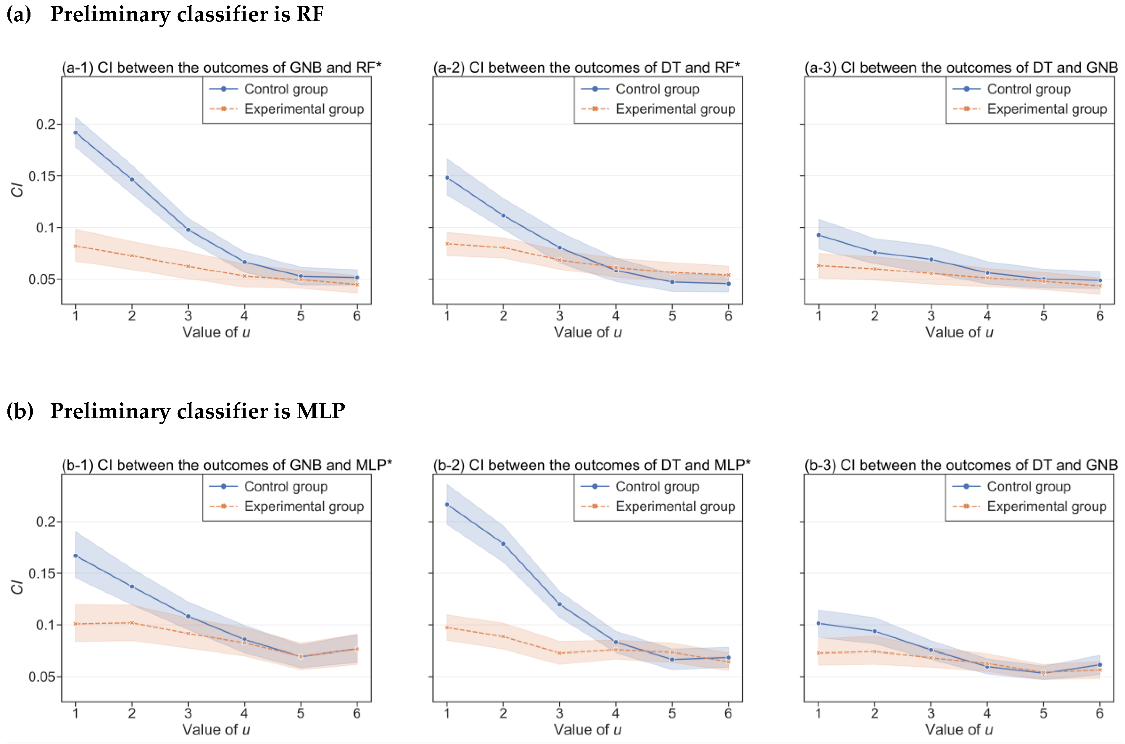
2.3. Testing Conditional Independence

Conditional independence is a crucial assumption in GLC-TCCA. To find out the optimal couple of classifiers that satisfied TCCA’s assumption on conditional independence, we need to first test the conditional independence among the local classification systems and the prediction. In this study, the degree of conditional independence was quantified based on the following equation:

$${\rho }_1=\frac{S_1^{*}-S_1^X{S}_1^Y}{\sqrt{S_1^X(1-S_1^X)S_1^Y(1-S_1^Y)}}$$

(10)

for the target class and

$${\rho }_0=\frac{S_0^{*}-S_0^X{S}_0^Y}{\sqrt{S_0^X(1-S_0^X)S_0^Y(1-S_0^Y)}}$$

(11)

for the rest data in the dichotomous problem. The superscripts X and $Y$ denote the two classification systems to be compared. $S_1^{*}=P(X=1,Y=1|\mathsf{\Theta }=1)$ and $S_0^{*}=P(X=0,Y=0|\mathsf{\Theta }=0)$. When ${\rho }_1$ and ${\rho }_0$ are substantially close to 0, the classification system X and Y could be considered conditionally independent [56,61,62]. For simplicity, we defined a single indicator $CI$ to quantify the correlation independence between two classification systems:

$$CI=\sqrt{\left|{\rho }_1{\rho }_0\right|}$$

(12)

3. Experiments

Three experiments were sequentially conducted in this article. The first experiment (Section 3.1) tested the sensitivity of TCCA when data were significantly imbalanced. The results would be beneficial in determining the minimum proportion of sample size that could be handled by TCCA in a reliable manner. The second experiment (Section 3.2) was designed to test the influences of different couples of local classifiers and to determine the optimal parameter in the Gaussian density function. The third experiment (Section 3.3) demonstrated the practices of GLC-TCCA on real-life GLC assessment.

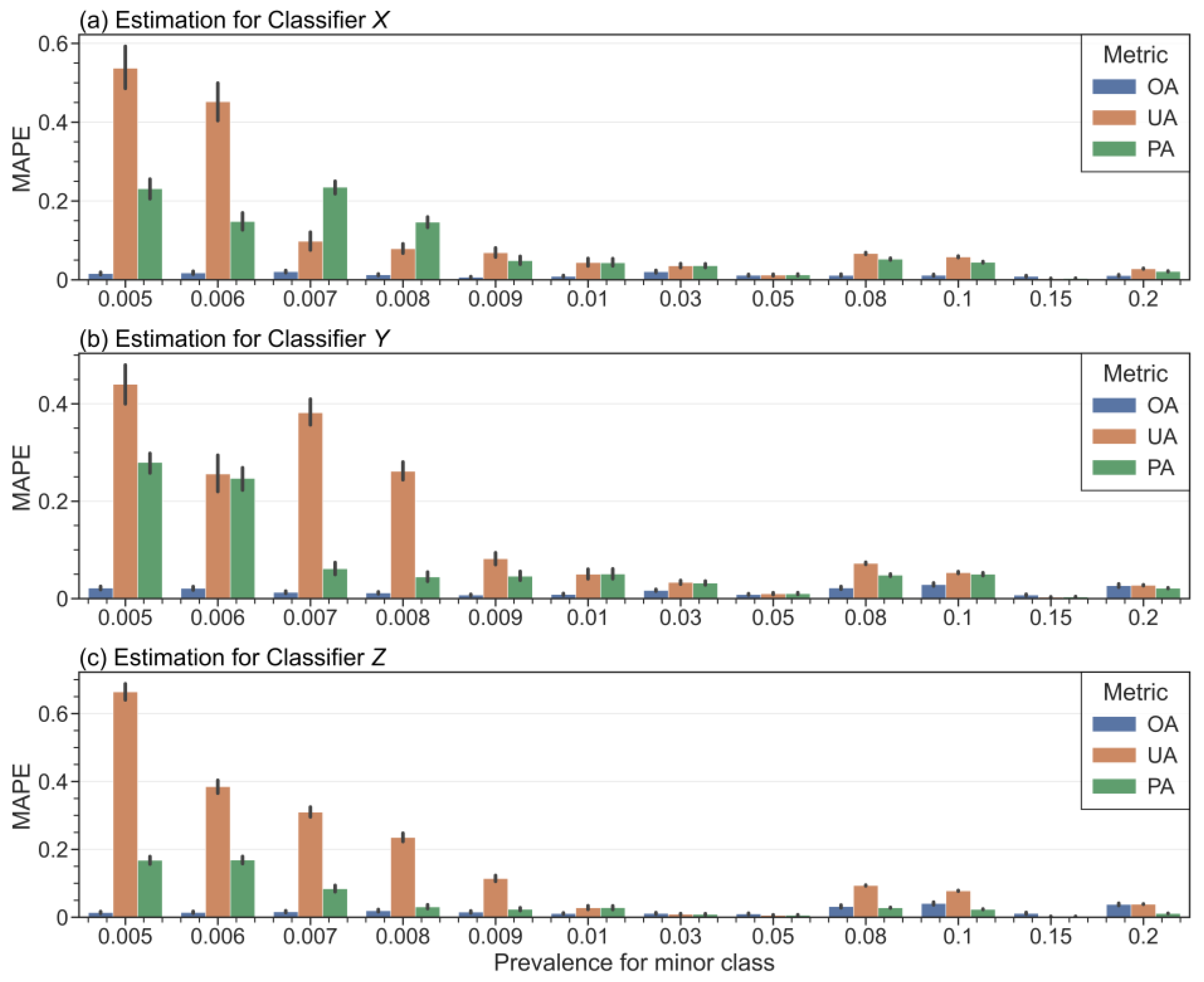
3.1. Sensitivity of TCCA on Extremely Imbalanced Data

TCCA has been proven to be unbiased in addressing moderately unbalanced data (e.g., when the prevalence is 0.8 and 0.2 for two classes) [41]. However, given that data can be extremely unbalanced in GLC (e.g., built-up accounts for only 0.7% in WorldCover 2020), to what extent TCCA can deal with such unbalance should be further explored.

In this section, we reconsidered the scenario simulated in the original paper of TCCA, in which three classifiers X, Y and Z, with a false alarm rate and misdetection rates of (8%,12%), (10%, 30%) and (20%, 40%), respectively, were applied to unbalanced data with 4000 sample points (3200 for class 1 and 800 for class 2) [41]. We examined the effectiveness of TCCA by varying the prevalence of class 2 from 0.2 to 0.005. Particularly, as the uncertainty of TCCA would be large with a small sample size (e.g., less than 1000), we reset the total number of simulated samples to 400,000 and fixed the sampling rate to 0.5. Thus, each test had at least 1000 points for the minor class. Furthermore, we monitored the estimation of commonly used metrics, including OA, PA and UA, in terms of their mean absolute percentage error (MAPE) in this experiment. Mathematically, MAPE could be written as:

$$MAPE=\frac{\left|Y-\widehat{Y}\right|}{Y}$$

(13)

where $\widehat{Y}$ is the estimate, and $Y$ is the actual value.

The results of the MAPE measurements for different accuracy metrics are shown in Figure 2. TCCA achieved especially low MAPE for OA in all the cases, whereas the estimations of PA and UA were less accurate and indicated large deviations when the minor class was assigned a prevalence lower than 0.01. When the size of the minor class is reduced to a comparable magnitude to the model uncertainty of TCCA, even a slight error in estimating the element of the confusion matrix will introduce significant deviations for PA and UA of the minor class. The estimation for OA is more stable than the one for other metrics because OA in an unbalanced scenario is primarily determined by the true-positive number of the major class, which would not change significantly because of the relatively small error in the elements of the confusion matrix. Thus, to maintain the reliability of the results, we skipped the estimation of classes with a prevalence lower than 0.01 and focused on the OA estimation in the following experiments. It is also noteworthy that, according to the study of Pierdicca et al. [41], TCCA becomes less stable when the sample size is small. Therefore, we further excluded the estimation of classes with a sample size lower than 100 to control the reliability in the following experiments.

3.2. Tuning GLC-TCCA on a Real-Life Dataset with Known Ground Truth

3.2.1. Experimental Setup

In this section, we used LCN-AFR to test the performance of our proposed approach and tune parameters for the further case study. LCN-AFR is an annual training dataset at a 10 m resolution for land cover classification, which consists of 1980 chips of $256\times 256$ pixels across 89 tiles ($3\times 3$ degree) in Africa [63]. The whole dataset was produced under a seven-class scheme and manually validated by three independent experts. More details on LCN-AFR can be found in Alemohammad and Booth (2020) [63]. The present study filtered the most reliable pixels with a consensus score of 100, which can be used as ground truth for validation. Furthermore, to save the computational cost, we randomly sampled 5% from the filtered result and finally obtained a collection of over 3.8 million pixels for further experiments.

The workflow of this experiment is shown in Figure 3. Firstly, we trained a preliminary classifier based on 5% random pixels and the Sentinel-2 time series associated with each chip in LCN-AFR. A total of 240 spectral features were extracted from the Sentinel-2 images, following the instructions in the original paper on LCN-AFR [63]. Then, the trained preliminary classifier was applied to the whole collection to generate predictions for each pixel. Finally, we applied GLC-TCCA to the prediction in each tile, following the strategies introduced in Section 2.2. Additional concerns were given to explore the influence of two initial conditions for TCCA in this experiment, including the choice of classifiers and the parameter $u$ in Gaussian density function used for sample collection. It is worth noting that tree-based models and neural network (NN) are widely used in GLC mapping [6,9], and we selected two representative methods, namely, the random forest model (RF) (Scenario A) and the Multi-layer Perceptron classifier (MLP) (Scenario B), as the preliminary classifiers. This allowed us to test our methods under different scenarios.

3.2.2. Choice of Classifiers

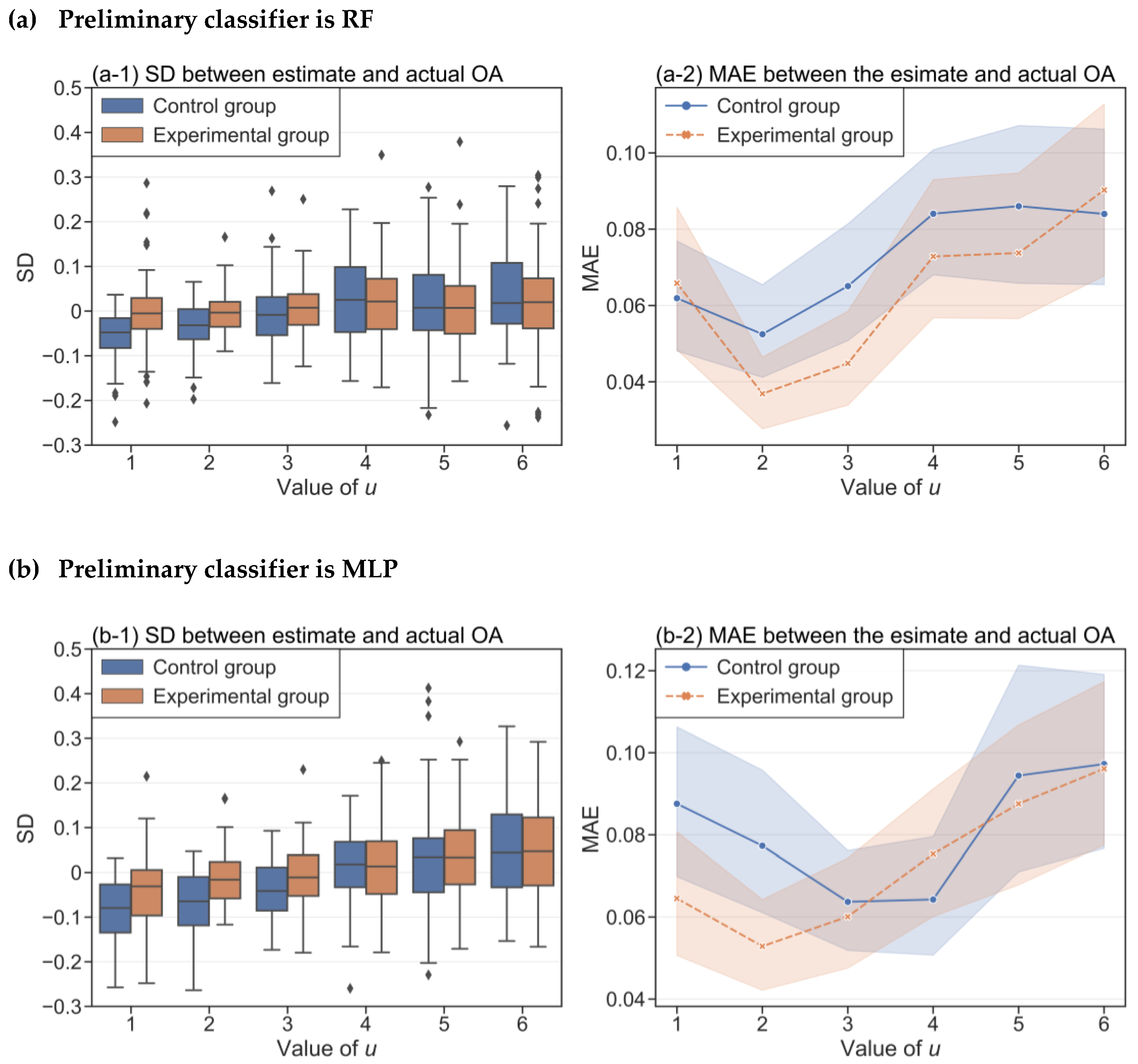
We chose four basic classifiers as candidates for the two local classifiers in this study, including decision tree (DT), random forest (RF), support vector machine (SVM), and Gaussian Naive Bayes (GNB).

We ranged the parameter $u$ from 1 to 6. We first calculated the CI values between the systems produced by each classifier and the prediction. Notably, considering the computation cost and effectiveness of training, a balanced training set of 10,000 points (i.e., 5000 for the target class and 5000 for the rest) was selected during the training of the local classifier for each land class.

As shown in

Table 1. Statistics of $CI$ between the system produced by different local classifiers and values of $u$. Std refers to standard deviation.

Preliminary Classifier	Sampling Parameter	Local Classifier
		DT		RF		SVM		GNB
		Mean	Std	Mean	Std	Mean	Std	Mean	Std
RF	$u=1$	0.084	0.042	0.411	0.117	0.387	0.114	0.082	0.057
	$u=2$	0.081	0.037	0.408	0.112	0.375	0.112	0.073	0.050
	$u=3$	0.068	0.036	0.391	0.108	0.361	0.108	0.062	0.047
	$u=4$	0.061	0.035	0.349	0.103	0.326	0.116	0.053	0.040
	$u=5$	0.056	0.033	0.327	0.123	0.298	0.115	0.050	0.032
	$u=6$	0.054	0.031	0.311	0.125	0.284	0.123	0.045	0.030
MLP	$u=1$	0.097	0.047	0.459	0.118	0.530	0.116	0.010	0.065
	$u=2$	0.088	0.044	0.466	0.113	0.523	0.121	0.010	0.062
	$u=3$	0.073	0.041	0.441	0.105	0.493	0.124	0.092	0.052
	$u=4$	0.076	0.032	0.404	0.122	0.451	0.119	0.082	0.050
	$u=5$	0.073	0.035	0.362	0.147	0.406	0.151	0.070	0.046
	$u=6$	0.064	0.031	0.344	0.155	0.386	0.146	0.076	0.052

, DT and GNB show a lower average value of $CI$ (<0.1) in all cases, whilst the values associated with RF and SVM are substantially larger than 0, which indicates that RF and SVM might not satisfy the assumption of conditional independence in TCCA. To further test the applicability of GNB and DT, we calculated the $CI$ between them. Additionally, to demonstrate the effectiveness of the exclusion of assessed tile when constructing the neighbourhood set, we created a control group in which the assessed tile was included in the neighbourhood set and recorded the corresponding $CI$ values. As shown in Figure 4, the exclusion of the assessed tile from the neighbourhood set could significantly reduce the $CI$ values, especially when the parameter $u$ is small. When $u$ became larger, the Gaussian density function would assign less weight to the assessed tile in the control group. Therefore, the difference in $CI$ between the control and experimental group would diminish. Moreover, it can be seen in Figure 4(a-3,b-3) that the increment of $CI$ in control group is relatively smaller than those in other scenarios, which indicates that the errors in the outcomes of the selected local classifiers tend to be uncorrelated even though the training sample might inherit some errors from the assess tiles.

According to the superior performance in the simulation, DT and GNB were selected as the two local classifiers for the following experiments:

3.2.3. Selection of the Parameter $u$ in the Gaussian Density Function

To choose the optimal value of $u$ in the Gaussian density function, we investigated the influence of different values of $u$ on estimation accuracy. The resultant estimations were evaluated in terms of the mean absolute error (MAE) and signed deviation (SD), which are expressed as follows:

$$\begin{array}{l}\mathrm{MAE}(\widehat{\theta })=\frac{1}{n}{\displaystyle \sum _{i=1}^n\left|{\theta }_i-\widehat{{\theta }_i}\right|}\\ \mathrm{SD}(\widehat{\theta })={\theta }_i-\widehat{{\theta }_i}\end{array}$$

(14)

where $\widehat{{\theta }_i}$ refers to the estimate of the true accuracy metric ${\theta }_i$ (e.g., OA) of grid $i$. Compared with MAE, which measures the average magnitude of errors in the estimates, the mean of SD (MSD) captures the average differences between truth and estimate. An MSD value smaller than zero may imply a general overestimation.

As shown in Figure 5(a-1,b-1), overestimations can be observed in the control group in terms of their MSD substantially lower than 0 when $u$ is small (e.g., $u=1$ or 2). The reason could be that local classifiers tend to inherit classification errors from the assessed tile in the control group. As a result, the local classifiers would produce similar predictions that contain correlated errors to the data being evaluated. According to Pierdicca et al. (2017) [41], such a correlation would lead to overestimating the accuracy of systems with similar outcomes. This inference is also supported by Table 1 and Figure 4 as the highest values of $CI$ generally appear at $u=1$. In contrast, the overestimation was largely reduced with the exclusion of the assessed tile as the MSD is close to 0 in the experimental group. These findings, again, justify the construction of the neighbourhood set in this study.

As shown in Figure 5(a-2,b-2), the MAE of the estimation declines at first and then increases with the increment of $u$. This can also be explained by the fact that the local classifiers tend to inherit errors that might be correlated to those in the assessed tile when the training sample concentrates in a low-order neighbourhood. However, when $u$ becomes too large, the effectiveness of local classifiers is lowered. As TCCA generally trusts the systems that present similar outcomes more [41], TCCA would judge the target system (i.e., the outcome of the preliminary classifier) to be less accurate when it is significantly different to the other two local systems. In sum, regardless of the preliminary classifier used, the smallest MAE always appear at $u=2$. Therefore, given that LCN-AFR has very similar data properties (e.g., resolution and classification scheme) to WorldCover 2020, we finally adopted $u=2$ in the Gaussian density function and used DT and GNB as the local classifiers in the following experiments on WorldCover 2020.

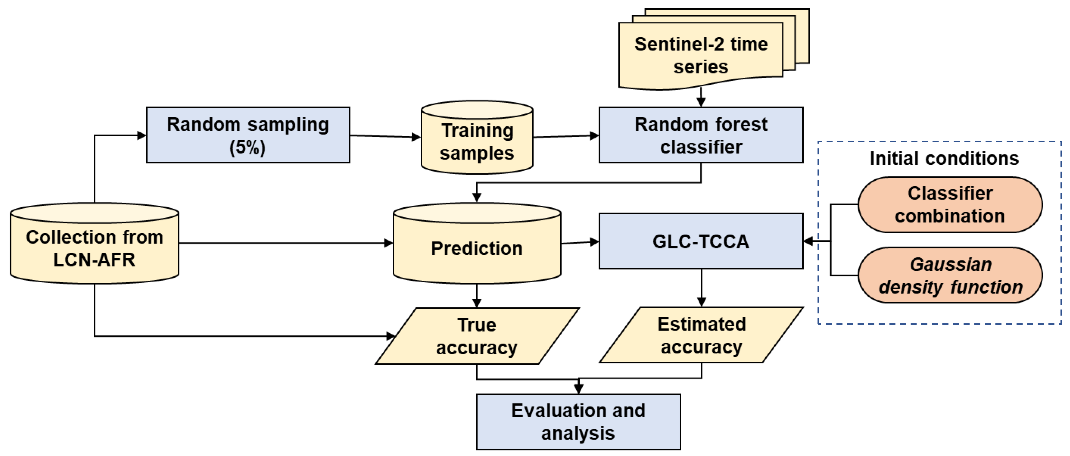
3.3. GLC-TCCA Applied to WorldCover 2020

In this section, we demonstrated the performance of GLC-TCCA on WorldCover 2020, a 10 m resolution GLC dataset produced by ESA. WorldCover 2020 is claimed to have an overall accuracy of 74.4%. WorldCover 2020 is also available on GEE, which significantly offers easy access and data processing. Details about the accuracy of WorldCover 2020 can be found in the European Space Agency (2021) [64].

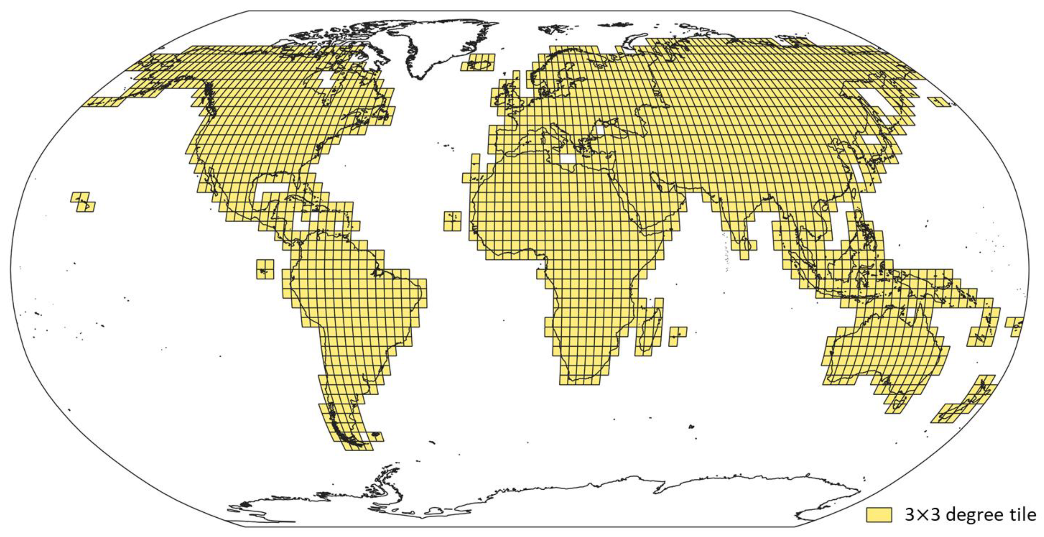
3.3.1. Data Preparation

To generate a sufficient number of global sample points for applying GLC-TCCA, we randomly picked points based on a density of approximately one point per 9 km², considering memory and computation limitations in GEE. To train the local classifiers, a total of 98 remote sensing features were extracted from Sentinel-1 (S1), Sentinel-2 (S2) and AW3D30 Version 3.2. Details of the feature extraction could be found in the Supplementary file. It should be noted that different feature combinations are expected to influence the results of GLC-TCCA, however, exploring the best combination is out of the scope of this study.

Given that S1 and S2 do not cover the full surface of the Earth, some sample points would be invalid because of the lack of image coverage. Thus, they were discarded in this study. For example, Greenland and the northernmost regions of Canada were excluded from this study due to the lack of S1 images in VV-VH mode. Finally, we obtained over 15 million points covering 2207 $3\times 3$ degree tiles (Figure 6) for the following experiments.

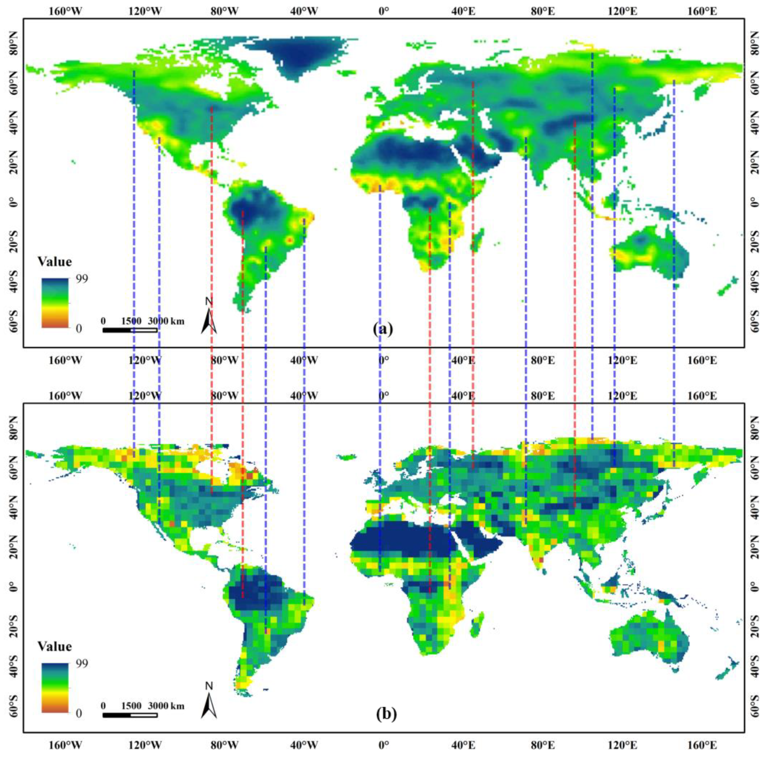
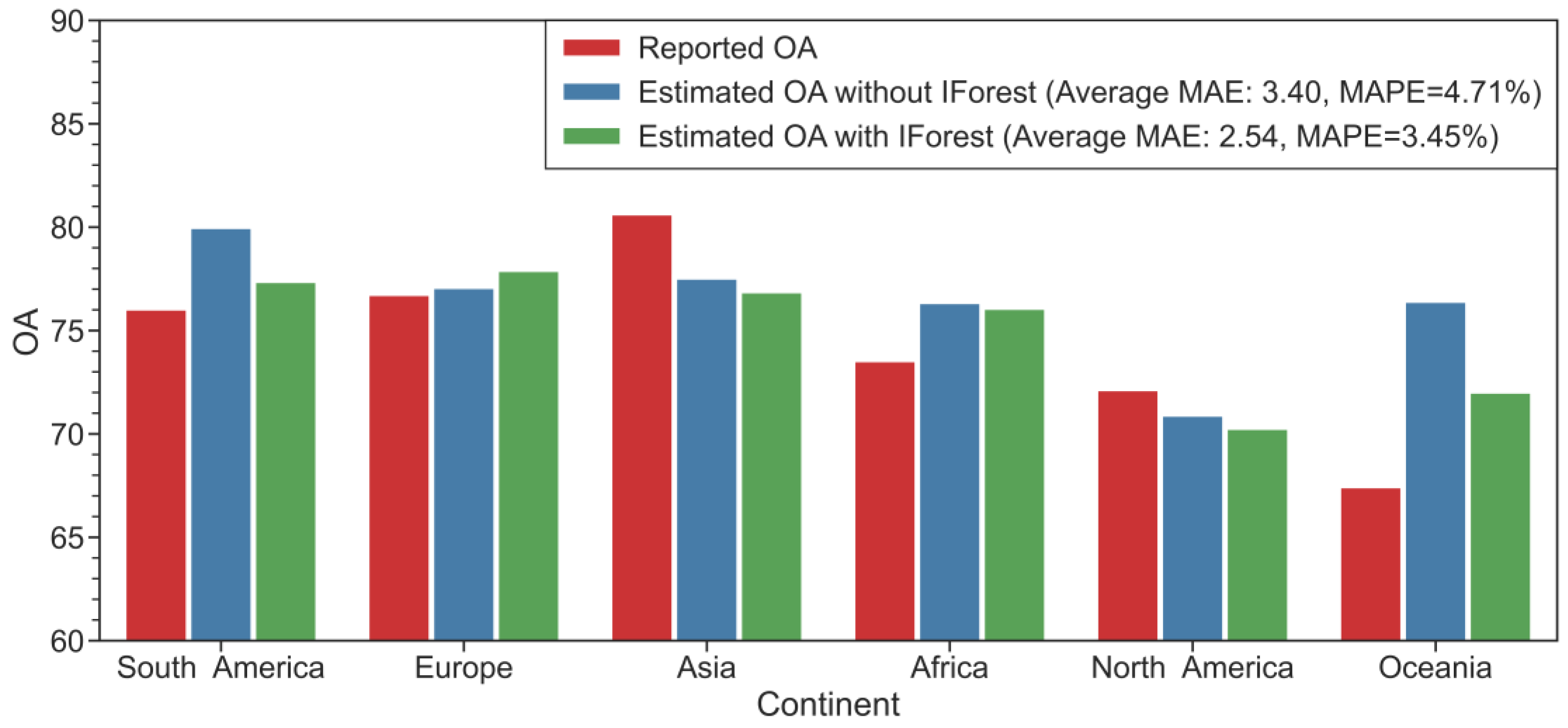
3.3.2. Estimation of WorldCover 2020 at the Continent Level

Given the lack of rigorous reference data (i.e., grid-specific accuracy information) for WorldCover 2020, we utilised the accuracy information for each continent and the global accuracy map reported in the product report of WorldCover 2020 to verify the performance of our method.

The accuracy map estimated by GLC-TCCA and the official one are compared in Figure 7. Given that numeric data are unavailable for the official accuracy map, we cannot make a direct quantitative comparison. However, through a quick visual comparison, we found that the estimation of GLC-TCCA captured most of the spatial patterns of the accuracy map. For example, significant high-accuracy areas (connected by a blue dashed line) and low-accuracy areas (connected by a red dashed line) were successfully identified by GLC-TCCA. The estimated OA values for each continent are summarised in

Table 2. Comparison of the reported and estimated OA at the continent level.

Continent	Reported OA (Official)	Estimated OA	Absolute Error	Absolute Percentage Error
South America	76.10	80.04	3.94	5.18%
Europe	76.80	77.14	0.34	0.44%
Asia	80.70	77.59	5.11	3.85%
Africa	73.60	76.41	2.81	3.82%
North America	72.20	70.96	1.24	1.71%
Oceania	67.50	76.47	8.97	13.29%
Average			3.40	4.71%

. In most cases, the estimations of GLC-TCCA are close to the reported OA provided by ESA, with a mean absolute error (MAE) of 3.40, and a mean absolute percentage error (MAPE) of 4.71%. These findings prove the effectiveness of the proposed GLC-TCCA in providing a generally reliable estimation and capturing the most spatial variation of the accuracy of WorldCover 2020.

There are at least two reasons that explain the mismatches between Figure 7a and Figure 6b: (1) Model errors exist in the results of GLC-TCCA, and (2) Given that two accuracy layers are produced with different spatial resolutions (i.e., 100 m for (a) and $3\times 3$ degree tile for (b)), some local extremum in (a) tend to be smoothed in (b), which is believed to cause a certain level of mismatch, such as the one in eastern South America.

It is noteworthy that certain grids at high latitudes have smaller areas due to the distortion caused by projection and occupation by the sea, resulting in their reduced weights in the calculation of overall accuracy. The northeast regions of North America, for instance, visually exhibit a greater difference in accuracy; however, this does not significantly diminish the overall accuracy of North America, as shown in Table 2.

The largest absolute error was observed in the estimation of Oceania. The reason for the relatively lower effectiveness of GLC-TCCA in Oceania are as follows: (1) A large proportion of grids in Oceania is close to the sea, and their neighbourhoods are relatively broken, containing fewer neighbouring tiles than the ones in other continents. As shown in

Table 3. Number of neighbours in the neighbourhood set ${\mathsf{\Phi }}_9$ at the continent level.

Continent	Average Number of Neighbouring Tiles
South America	172
Europe	245
Asia	255
Africa	237
North America	196
Oceania	146
Global	223

, the average number of neighbours of Oceania is only 146, which is significantly lower than the global average of 223. In that sense, sample points might concentrate in low-order neighbourhoods, and an overestimation could be expected, as discussed in Section 3.2. The same issue also occurs in South America, where the number of neighbours is only 172. (2) As Oceania presents the lowest true OA of 67.5% among all the continents, sample points from the neighbourhood set are more likely to be wrongly labelled. Thus, classifications produced by local classifiers tend to inherit more correlated errors from the original data, which is expected to result in an overestimation, according to Pierdicca et al. [41].

3.3.3. Improving GLC-TCCA with the Screening of Reliable Sample

The final section verifies the feasibility and effectiveness of the proposed GLC-TCCA. However, as mentioned above, some estimates are less reliable because of the high proportion of erroneous sample points. To that end, we added an outlier detection phase based on isolation forest (IForest) for the filtration of reliable sample points before training local classifiers. Compared with other outlier detection techniques, IForest has been proven robust and efficient in handling large data volumes and high-dimensional problems given its ensemble framework and nearly linear complexity [65].

For GLC data, erroneous pixels may be limited to common outliers that present abnormal dispersions from others and possibly form clusters when the number of errors reaches a certain level. In this regard, we discarded the top 10% sample points in the anomaly score estimated by IForest. We chose 10% as the threshold because OA for GLC products is commonly around 80, and we conservatively assumed that 50% of the errors might form clusters. Thus, the remaining sample can still capture most land characteristics that allow training effective local classifiers.

As shown in Figure 8, the overestimation of OA in Oceania and South America was significantly reduced, whereas the estimated accuracy of other continents remained consistent with the previous estimates that were produced without IForest. After using IForest, the MAE was reduced from 3.40 to 2.54, and MAPE was reduced from 4.71% to 3.45%.

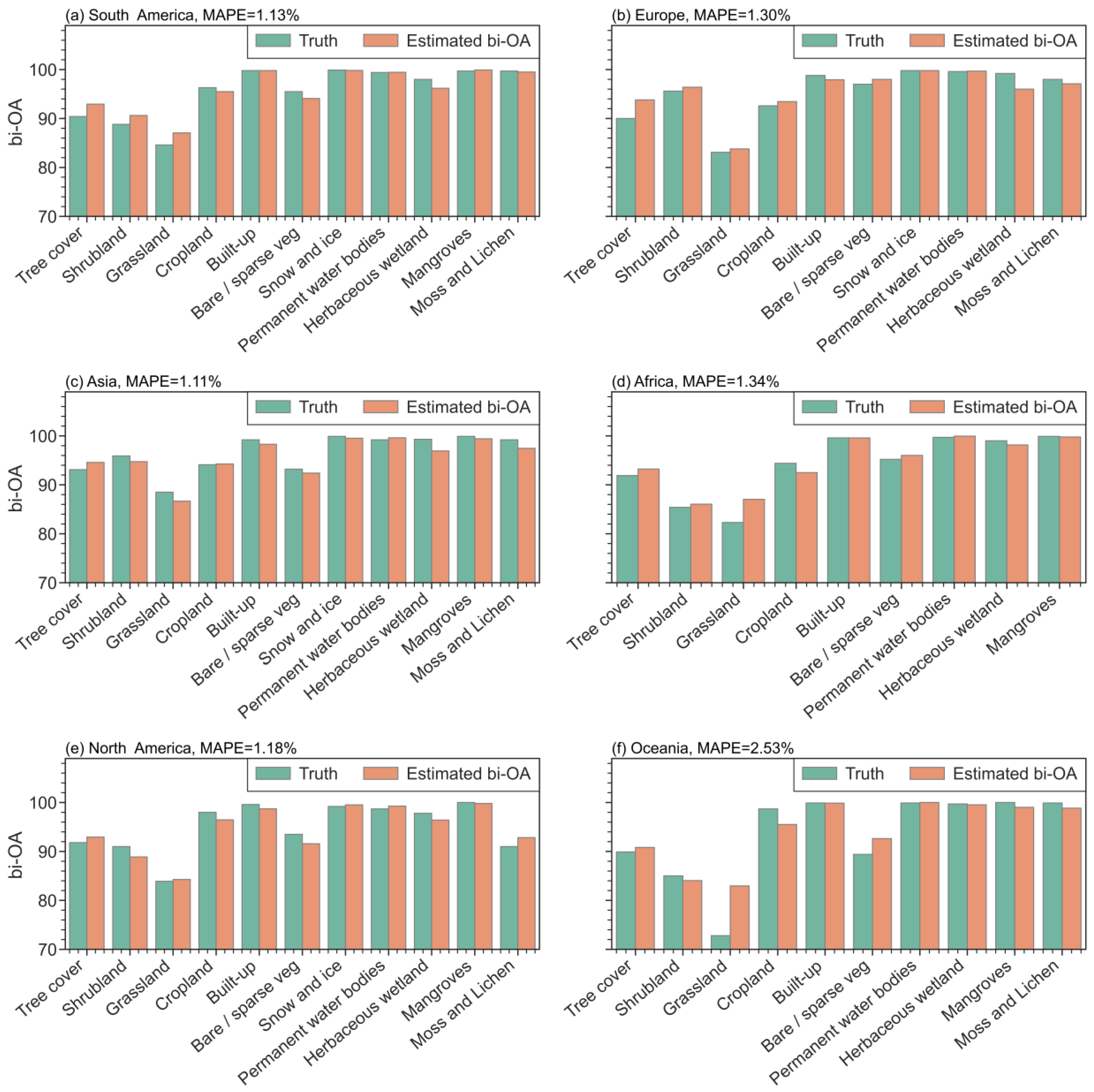
3.3.4. Class-Specific Accuracy Analysis Based on the Estimates of Improved GLC-TCCA

We further calculated the bi-OA for each class based on Equation (8) and compared the result with its truth derived from the product report of WorldCover 2020. As shown in Figure 9, the low value of MAPE for each continent proves the general correctness of the bi-OA estimates. However, deviations can be observed in some minor classes, such as Moss and Lichen in Asia (0.71% of the original data in Asia) and Herbaceous wetland in Europe (0.71% of the original data in Europe). As discussed in Section 3.1, lower prevalence will result in a larger deviation when solving the binary-classification problem using TCCA. However, these deviations would have less effect on the estimation of the entire dataset because the absolute sample sizes of these classes are small.

The most significant deviation seems to occur in the Grassland of Oceania. According to the product report of WorldCover 2020, the true bi-OA of Grassland in Oceania was computed to be 72%, which is the lowest among all the cases we considered in Figure 9. Therefore, approximately 28% of the samples are erroneous when training the local classifiers to evaluate the accuracy of Grassland. Although IForest was applied to reduce the influence of the errors from the original data, the influence cannot be fully avoided when the quantity of erroneous pixels is too large. Furthermore, Grassland accounts for 54.64% of the original data in Oceania. This low accuracy of Grassland and its high proportion in Oceania would increase the error correlation between the three input systems for GLC-TCCA and thus result in less reliable estimates.

4. Discussion

The essence of GLC-TCCA is to estimate the confusion matrixes of multiple classifications based on their agreements. The overall correctness of the data should be carefully checked before applying GLC-TCCA in practice. The estimation could be invalid if the accuracy of the original data is too low. In that situation, both local classifiers are likely to produce erroneous predictions, which will lead to a high proportion of correlated errors between local classifications and thus violate the assumption of their conditional independence given the ground truth. However, given that the majority of existing GLC data are reported to have a similar OA to WorldCover 2020, which is over 70%, we believe GLC-TCCA could also apply to most GLC products, given its performance in WorldCover 2020.

It is important to note that the accuracy of each classification does not affect the results of GLC-TCCA, as long as the assumption of conditional independence is satisfied [41]. In this study, the construction of neighbourhoods plays a crucial role in consolidating this assumption by enabling the utilization of spatial heterogeneity to reduce the potential dependency between the assessed data and local classifications. This step also ensures the effectiveness of local classifiers by using local samples and avoiding potential correlation between local classifications caused by very low accuracy as discussed above. In addition, we weakened the impact of classification errors on local classifiers by screening reliable samples and conducting multiple times of training, which would further reduce the potential dependency between the original data and local classifications. The effectiveness of these operations was demonstrated by the significantly reduced CI values shown in Figure 4 and the improved estimates shown in Figure 8.

The computational cost could be a critical concern when using GLC-TCCA in practice. Retrieving massive global sample points with their spectral and terrain features is the first step for conducting GLC-TCCA. Fortunately, with the help of modern cloud computing platforms, such as GEE, the remote sensing data processing cost can be largely reduced. Furthermore, although GLC-TCCA involves many computational procedures, such as training local classifiers and outlier detectors, its ensemble framework makes most of these procedures parallelisable. Thus, the time cost can be greatly reduced by distributing the estimation task.

5. Conclusions

While various GLC products are rapidly produced and updated with advanced classification techniques, their assessment seems to “fall behind” in providing timely accuracy reports to support decision-making. Despite the high reliability, traditional sample-based assessment approaches are often restrained by the lack of ground truth and criticised for the huge workload and low efficiency. This study develops a new reference-free method termed GLC-TCCA, particularly for estimating the thematic accuracy of GLC products. Compared with traditional assessment methods that rely heavily on ground reference data, GLC-TCCA makes full use of the original classification information and does not rely on any external data except remote sensing images. According to the experiment on WorldCover 2020, GLC-TCCA can provide accurate estimates for individual land classes and the whole dataset at the continent level with a relative error of approximately 4%.

The reference-free characteristics of GLC-TCCA make it a useful tool for GLC producers and users. From the producers’ perspective, GLC-TCCA allows a quick survey of spatial accuracy of large-scale land cover datasets without conducting situ measurement. Furthermore, the spatial accuracy layer produced by GLC-TCCA is valuable for producers to target poorly classified regions and thus take more efficient interventions (e.g., training sophisticated local classification models or scrutinising poorly classified regions) to improve the data accuracy before delivery to the users. From users’ perspective, the results of GLC-TCCA could serve as a third-party inspection to validate the reported accuracy of land cover data and allow users’ self-services to obtain classification accuracy, which is only empirically estimated and reported by the producers.

Improvements can be made in future works. Firstly, as many grid cells are located on the edge of a continent or island, their neighbours’ actual number and spatial coverage could be significantly smaller than those located in the land’s interior. To address that issue, adaptive neighbourhoods could be developed to train better local classifiers. Secondly, only spectral and terrain features are used in this study. Given the massive land classification information in existing GLC data and crowdsourcing data, how auxiliary information could be used to enhance GLC-TCCA needs to be further explored. Thirdly, the effect of the accuracy of the original data on the reliability of estimations needs to be further quantified by experiments and simulations. Lastly, stable and efficient software needs to be developed in future work to enhance the practical utilisation of GLC-TCCA.

References

1. Gong, P.; Zhang, W.; Yu, L.; Li, C. New research paradigm for global land cover mapping. J. Remote Sens. 2016, 20, 1002–1016. [Google Scholar] [CrossRef]
2. Loveland, T.R.; Reed, B.C.; Brown, J.F.; Ohlen, D.O.; Zhu, Z.; Yang, L.; Merchant, J.W. Development of a global land cover characteristics database and IGBP DISCover from 1 km AVHRR data. Int. J. Remote Sens. 2000, 21, 1303–1330. [Google Scholar] [CrossRef]
3. Bossard, M.; Feranec, J.; Otahel, J. CORINE Land Cover Technical Guide: Addendum 2000; European Environment Agency: Copenhagen, Denmark, 2000. [Google Scholar]
4. Brown, C.F.; Brumby, S.P.; Guzder-Williams, B.; Birch, T.; Hyde, S.B.; Mazzariello, J.; Czerwinski, W.; Pasquarella, V.J.; Haertel, R.; Ilyushchenko, S.; et al. Dynamic World, Near real-time global 10 m land use land cover mapping. Sci. Data 2022, 9, 251. [Google Scholar] [CrossRef]
5. Chen, J.; Chen, J.; Liao, A.; Cao, X.; Chen, L.; Chen, X.; He, C.; Han, G.; Peng, S.; Lu, M.; et al. Global land cover mapping at 30 m resolution: A POK-based operational approach. ISPRS J. Photogramm. Remote Sens. 2015, 103, 7–27. [Google Scholar] [CrossRef]
6. Gong, P.; Wang, J.; Yu, L.; Zhao, Y.; Zhao, Y.; Liang, L.; Niu, Z.; Huang, X.; Fu, H.; Liu, S.; et al. Finer resolution observation and monitoring of global land cover: First mapping results with Landsat TM and ETM+ data. Int. J. Remote Sens. 2013, 34, 2607–2654. [Google Scholar] [CrossRef]
7. Hansen, M.C.; Potapov, P.V.; Pickens, A.H.; Tyukavina, A.; Hernandez-Serna, A.; Zalles, V.; Turubanova, S.; Kommareddy, I.; Stehman, S.V.; Song, X.-P.; et al. Global land use extent and dispersion within natural land cover using Landsat data. Environ. Res. Lett. 2022, 17, 034050. [Google Scholar] [CrossRef]
8. Belward, A.S.; Skøien, J.O. Who launched what, when and why; trends in global land-cover observation capacity from civilian earth observation satellites. ISPRS J. Photogramm. Remote Sens. 2015, 103, 115–128. [Google Scholar] [CrossRef]
9. Li, X.; Chen, G.; Liu, X.; Liang, X.; Wang, S.; Chen, Y.; Pei, F.; Xu, X. A New Global Land-Use and Land-Cover Change Product at a 1-km Resolution for 2010 to 2100 Based on Human–Environment Interactions. Ann. Assoc. Am. Geogr. 2017, 107, 1040–1059. [Google Scholar] [CrossRef]
10. Mantyka-Pringle, C.S.; Visconti, P.; Di Marco, M.; Martin, T.G.; Rondinini, C.; Rhodes, J.R. Climate change modifies risk of global biodiversity loss due to land-cover change. Biol. Conserv. 2015, 187, 103–111. [Google Scholar] [CrossRef]
11. Straume, K. The social construction of a land cover map and its implications for Geographical Information Systems (GIS) as a management tool. Land Use Policy 2014, 39, 44–53. [Google Scholar] [CrossRef]
12. Congalton, R.G.; Gu, J.; Yadav, K.; Thenkabail, P.; Ozdogan, M. Global Land Cover Mapping: A Review and Uncertainty Analysis. Remote Sens. 2014, 6, 12070–12093. [Google Scholar] [CrossRef]
13. Chen, P.; Shi, W.; Kou, R.; Wan, Y. A quantitative investigation of the uncertainty associated with mapping scale in the production of land-cover/land-use data. Int. J. Remote Sens. 2018, 39, 8798–8817. [Google Scholar] [CrossRef]
14. Tchuente, A.T.K.; Roujean, J.-L.; Faroux, S. ECOCLIMAP-II: An ecosystem classification and land surface parameters database of Western Africa at 1km resolution for the African Monsoon Multidisciplinary Analysis (AMMA) project. Remote Sens. Environ. 2010, 114, 961–976. [Google Scholar] [CrossRef]
15. Tsendbazar, N.; Herold, M.; Li, L.; Tarko, A.; de Bruin, S.; Masiliunas, D.; Lesiv, M.; Fritz, S.; Buchhorn, M.; Smets, B.; et al. Towards operational validation of annual global land cover maps. Remote Sens. Environ. 2021, 266, 112686. [Google Scholar] [CrossRef]
16. Nelson, M.D.; Garner, J.D.; Tavernia, B.G.; Stehman, S.V.; Riemann, R.I.; Lister, A.J.; Perry, C.H. Assessing map accuracy from a suite of site-specific, non-site specific, and spatial distribution approaches. Remote Sens. Environ. 2021, 260, 112442. [Google Scholar] [CrossRef]
17. Foody, G.M. Explaining the unsuitability of the kappa coefficient in the assessment and comparison of the accuracy of thematic maps obtained by image classification. Remote Sens. Environ. 2020, 239, 111630. [Google Scholar] [CrossRef]
18. Olofsson, P.; Foody, G.M.; Herold, M.; Stehman, S.V.; Woodcock, C.E.; Wulder, M.A. Good practices for estimating area and assessing accuracy of land change. Remote Sens. Environ. 2014, 148, 42–57. [Google Scholar] [CrossRef]
19. Zhao, Y.; Gong, P.; Yu, L.; Hu, L.; Li, X.; Li, C.; Zhang, H.; Zheng, Y.; Wang, J.; Zhao, Y.; et al. Towards a common validation sample set for global land-cover mapping. Int. J. Remote Sens. 2014, 35, 4795–4814. [Google Scholar] [CrossRef]
20. Stehman, S.V.; Foody, G.M. Key issues in rigorous accuracy assessment of land cover products. Remote Sens. Environ. 2019, 231, 111199. [Google Scholar] [CrossRef]
21. Chen, P.; Huang, H.; Shi, W. Reference-free method for investigating classification uncertainty in large-scale land cover datasets. Int. J. Appl. Earth Obs. Geoinf. 2022, 107, 102673. [Google Scholar] [CrossRef]
22. Fonte, C.C.; Martinho, N. Assessing the applicability of OpenStreetMap data to assist the validation of land use/land cover maps. Int. J. Geogr. Inf. Sci. 2017, 31, 2382–2400. [Google Scholar] [CrossRef]
23. Fritz, S.; See, L.; Perger, C.; McCallum, I.; Schill, C.; Schepaschenko, D.; Duerauer, M.; Karner, M.; Dresel, C.; Laso-Bayas, J.-C.; et al. A global dataset of crowdsourced land cover and land use reference data. Sci. Data 2017, 4, 170075. [Google Scholar] [CrossRef] [PubMed]
24. Saah, D.; Johnson, G.; Ashmall, B.; Tondapu, G.; Tenneson, K.; Patterson, M.; Poortinga, A.; Markert, K.; Quyen, N.H.; Aung, K.S.; et al. Collect Earth: An online tool for systematic reference data collection in land cover and use applications. Environ. Model. Softw. 2019, 118, 166–171. [Google Scholar] [CrossRef]
25. Stehman, S.V.; Fonte, C.C.; Foody, G.M.; See, L. Using volunteered geographic information (VGI) in design-based statistical inference for area estimation and accuracy assessment of land cover. Remote Sens. Environ. 2018, 212, 47–59. [Google Scholar] [CrossRef]
26. Chen, J.; Chen, L.; Chen, F.; Ban, Y.; Li, S.; Han, G.; Tong, X.; Liu, C.; Stamenova, V.; Stamenov, S. Collaborative validation of GlobeLand30: Methodology and practices. Geo-Spat. Inf. Sci. 2021, 24, 134–144. [Google Scholar] [CrossRef]
27. Bayas, J.C.L.; See, L.; Bartl, H.; Sturn, T.; Karner, M.; Fraisl, D.; Moorthy, I.; Busch, M.; van der Velde, M.; Fritz, S. Crowdsourcing LUCAS: Citizens Generating Reference Land Cover and Land Use Data with a Mobile App. Land 2020, 9, 446. [Google Scholar] [CrossRef]
28. Bayas, J.C.L.; See, L.; Fritz, S.; Sturn, T.; Perger, C.; Dürauer, M.; Karner, M.; Moorthy, I.; Schepaschenko, D.; Domian, D.; et al. Crowdsourcing In-Situ Data on Land Cover and Land Use Using Gamification and Mobile Technology. Remote Sens. 2016, 8, 905. [Google Scholar] [CrossRef]
29. Fonte, C.C.; Antoniou, V.; Bastin, L.; Estima, J.; Arsanjani, J.J.; Bayas, J.-C.L.; See, L.; Vatseva, R. Assessing VGI Data Quality. In Mapping and the Citizen Sensor; Foody, G., See, L., Fritz, S., Mooney, P., Olteanu-Raimond, A.-M., Fonte, C.C., Antoniou, V., Eds.; Ubiquity Press: London, UK, 2017; pp. 137–163. [Google Scholar]
30. Koukoletsos, T.; Haklay, M.; Ellul, C. Assessing Data Completeness of VGI through an Automated Matching Procedure for Linear Data. Trans. GIS 2012, 16, 477–498. [Google Scholar] [CrossRef]
31. Gao, Y.; Liu, L.; Zhang, X.; Chen, X.; Mi, J.; Xie, S. Consistency Analysis and Accuracy Assessment of Three Global 30-m Land-Cover Products over the European Union using the LUCAS Dataset. Remote Sens. 2020, 12, 3479. [Google Scholar] [CrossRef]
32. Hua, T.; Zhao, W.; Liu, Y.; Wang, S.; Yang, S. Spatial Consistency Assessments for Global Land-Cover Datasets: A Comparison among GLC2000, CCI LC, MCD12, GLOBCOVER and GLCNMO. Remote Sens. 2018, 10, 1846. [Google Scholar] [CrossRef]
33. Pérez-Hoyos, A.; García-Haro, F.; San-Miguel-Ayanz, J. Conventional and fuzzy comparisons of large scale land cover products: Application to CORINE, GLC2000, MODIS and GlobCover in Europe. ISPRS J. Photogramm. Remote Sens. 2012, 74, 185–201. [Google Scholar] [CrossRef]
34. Liu, L.; Zhang, X.; Gao, Y.; Chen, X.; Shuai, X.; Mi, J. Finer-Resolution Mapping of Global Land Cover: Recent Developments, Consistency Analysis, and Prospects. J. Remote Sens. 2021, 2021, 5289697. [Google Scholar] [CrossRef]
35. Foody, G.M. Global and Local Assessment of Image Classification Quality on an Overall and Per-Class Basis without Ground Reference Data. Remote Sens. 2022, 14, 5380. [Google Scholar] [CrossRef]
36. Herold, M.; Mayaux, P.; Woodcock, C.; Baccini, A.; Schmullius, C. Some challenges in global land cover mapping: An assessment of agreement and accuracy in existing 1 km datasets. Remote Sens. Environ. 2008, 112, 2538–2556. [Google Scholar] [CrossRef]
37. Yang, H.; Li, S.; Chen, J.; Zhang, X.; Xu, S. The Standardization and Harmonization of Land Cover Classification Systems towards Harmonized Datasets: A Review. ISPRS Int. J. Geo-Inf. 2017, 6, 154. [Google Scholar] [CrossRef]
38. Radoux, J.; Defourny, P. Automated Image-to-Map Discrepancy Detection using Iterative Trimming. Photogramm. Eng. Remote Sens. 2010, 76, 173–181. [Google Scholar] [CrossRef]
39. Radoux, J.; Lamarche, C.; Van Bogaert, E.; Bontemps, S.; Brockmann, C.; Defourny, P. Automated Training Sample Extraction for Global Land Cover Mapping. Remote Sens. 2014, 6, 3965–3987. [Google Scholar] [CrossRef]
40. Chen, P.; Shi, W.; Kou, R. Reference-Free Measurement of the Classification Reliability of Vector-Based Land Cover Mapping. IEEE Geosci. Remote Sens. Lett. 2019, 16, 1090–1094. [Google Scholar] [CrossRef]
41. Pierdicca, N.; Anniballe, R.; Noto, F.; Bignami, C.; Chini, M.; Martinelli, A.; Mannella, A. Triple Collocation to Assess Classification Accuracy without a Ground Truth in Case of Earthquake Damage Assessment. IEEE Trans. Geosci. Remote Sens. 2017, 56, 485–496. [Google Scholar] [CrossRef]
42. Baraldi, A.; Bruzzone, L.; Blonda, P. Quality assessment of classification and cluster maps without ground truth knowledge. IEEE Trans. Geosci. Remote Sens. 2005, 43, 857–873. [Google Scholar] [CrossRef]
43. Steele, B.M. Maximum posterior probability estimators of map accuracy. Remote Sens. Environ. 2005, 99, 254–270. [Google Scholar] [CrossRef]
44. Foody, G.M. Latent Class Modeling for Site- and Non-Site-Specific Classification Accuracy Assessment without Ground Data. IEEE Trans. Geosci. Remote Sens. 2011, 50, 2827–2838. [Google Scholar] [CrossRef]
45. Stoffelen, A. Toward the true near-surface wind speed: Error modeling and calibration using triple collocation. J. Geophys. Res. Oceans 1998, 103, 7755–7766. [Google Scholar] [CrossRef]
46. Gruber, A.; Su, C.-H.; Crow, W.T.; Zwieback, S.; Dorigo, W.A.; Wagner, W. Estimating error cross-correlations in soil moisture data sets using extended collocation analysis. J. Geophys. Res. Atmos. 2016, 121, 1208–1219. [Google Scholar] [CrossRef]
47. Hoareau, N.; Portabella, M.; Lin, W.; Ballabrera-Poy, J.; Turiel, A. Error Characterization of Sea Surface Salinity Products Using Triple Collocation Analysis. IEEE Trans. Geosci. Remote Sens. 2018, 56, 5160–5168. [Google Scholar] [CrossRef]
48. Li, C.; Tang, G.; Hong, Y. Cross-evaluation of ground-based, multi-satellite and reanalysis precipitation products: Applicability of the Triple Collocation method across Mainland China. J. Hydrol. 2018, 562, 71–83. [Google Scholar] [CrossRef]
49. Gong, P.; Li, X.; Wang, J.; Bai, Y.; Chen, B.; Hu, T.; Liu, X.; Xu, B.; Yang, J.; Zhang, W.; et al. Annual maps of global artificial impervious area (GAIA) between 1985 and 2018. Remote Sens. Environ. 2019, 236, 111510. [Google Scholar] [CrossRef]
50. Zhang, X.; Liu, L.Y.; Wu, C.S.; Chen, X.D.; Gao, Y.; Xie, S.; Zhang, B. Development of a global 30 m impervious surface map using multisource and multitemporal remote sensing datasets with the Google Earth Engine platform. Earth Syst. Sci. Data 2020, 12, 1625–1648. [Google Scholar] [CrossRef]
51. Zhang, X.; Liu, L.; Chen, X.; Gao, Y.; Xie, S.; Mi, J. GLC_FCS30: Global land-cover product with fine classification system at 30 m using time-series Landsat imagery. Earth Syst. Sci. Data 2021, 13, 2753–2776. [Google Scholar] [CrossRef]
52. Zhu, Z.; Gallant, A.L.; Woodcock, C.E.; Pengra, B.; Olofsson, P.; Loveland, T.R.; Jin, S.; Dahal, D.; Yang, L.; Auch, R.F. Optimizing selection of training and auxiliary data for operational land cover classification for the LCMAP initiative. ISPRS J. Photogramm. Remote Sens. 2016, 122, 206–221. [Google Scholar] [CrossRef]
53. Arsanjani, J.J.; Tayyebi, A.; Vaz, E. GlobeLand30 as an alternative fine-scale global land cover map: Challenges, possibilities, and implications for developing countries. Habitat Int. 2016, 55, 25–31. [Google Scholar] [CrossRef]
54. Zhang, H.K.; Roy, D.P. Using the 500 m MODIS land cover product to derive a consistent continental scale 30 m Landsat land cover classification. Remote Sens. Environ. 2017, 197, 15–34. [Google Scholar] [CrossRef]
55. Tobler, W.R. A Computer Movie Simulating Urban Growth in the Detroit Region. Econ. Geogr. 1970, 46, 234–240. [Google Scholar] [CrossRef]
56. Foody, G.M. Assessing the accuracy of land cover change with imperfect ground reference data. Remote Sens. Environ. 2010, 114, 2271–2285. [Google Scholar] [CrossRef]
57. Tateishi, R.; Uriyangqai, B.; Al-Bilbisi, H.; Ghar, M.A.; Tsend-Ayush, J.; Kobayashi, T.; Kasimu, A.; Hoan, N.T.; Shalaby, A.; Alsaaideh, B. Production of Global Land Cover Data–GLCNMO. Int. J. Digit. Earth 2011, 4, 22–49. [Google Scholar] [CrossRef]
58. Yu, W.; Li, J.; Liu, Q.; Zeng, Y.; Zhao, J.; Xu, B.; Yin, G. Global Land Cover Heterogeneity Characteristics at Moderate Resolution for Mixed Pixel Modeling and Inversion. Remote Sens. 2018, 10, 856. [Google Scholar] [CrossRef]
59. Sahare, M.; Gupta, H. A Review of Multi-Class Classification for Imbalanced Data. Int. J. Adv. Comput. Res. 2012, 2, 160. [Google Scholar]
60. Chernoff, E.J. Sample space partitions: An investigative lens. J. Math. Behav. 2009, 28, 19–29. [Google Scholar] [CrossRef]
61. Branscum, A.; Gardner, I.; Johnson, W. Estimation of diagnostic-test sensitivity and specificity through Bayesian modeling. Prev. Veter-Med. 2005, 68, 145–163. [Google Scholar] [CrossRef]
62. Georgiadis, M.P.; Johnson, W.O.; Gardner, I.A.; Singh, R. Correlation-Adjusted Estimation of Sensitivity and Specificity of Two Diagnostic Tests. J. R. Stat. Soc. Ser. C 2003, 52, 63–76. [Google Scholar] [CrossRef]
63. Alemohammad, H.; Booth, K. LandCoverNet: A Global Benchmark Land Cover Classification Training Dataset. arXiv 2020, arXiv:2012.03111. [Google Scholar]
64. European Space Agency. Product Validation Report (D12-PVR); WorldCover_PVR_v1.0; European Space Agency: Paris, France, 2021. [Google Scholar]
65. Liu, F.T.; Ting, K.M.; Zhou, Z.-H. Isolation Forest. In Proceedings of the 2008 Eighth IEEE International Conference on Data Mining, Pisa, Italy, 15–19 December 2008; IEEE: Pisa, Italy, 2008; pp. 413–422. [Google Scholar]
Figure 1. Workflow of the proposed GLC-TCCA.
Remotesensing 15 02255 g001
Figure 2. Values of MAPE with different prevalence.
Remotesensing 15 02255 g002
Figure 3. Processes for tuning GLC-TCCA on LCN-AFR dataset.
Remotesensing 15 02255 g003
Figure 4. Statistics of CI between the preliminary classifier (i.e., RF or MLP) and local classifiers (i.e., DT and GNB) in different scenarios. * denotes the preliminary classifier.
Remotesensing 15 02255 g004
Figure 5. Accuracy evaluation of GLC-TCCA on LCN-AFR dataset under two different scenarios. DT and MLP were used as the local classifiers. The value of MSD is depicted by the horizontal line within the box in (a-1) and (b-1).
Remotesensing 15 02255 g005
Figure 6. Distribution of 3 × 3 degree tiles.
Remotesensing 15 02255 g006
Figure 7. Visual comparison between the official accuracy map of WorldCover 2020: (a) and the estimated one of GLC-TCCA (b). (a) is retrieved from the product validation report of WorldCover 2020. The red dashed lines connect areas with high accuracy in both (a) and (b), whilst the blue dashed lines connect those low-accuracy areas.
Remotesensing 15 02255 g007
Figure 8. Comparison of the estimates with and without using IForest for sample screening.
Remotesensing 15 02255 g008
Figure 9. Comparison of the reported and estimated class-specific accuracy at the continent level.
Remotesensing 15 02255 g009