Article

Efficient Deep Semantic Segmentation for Land Cover Classification Using Sentinel Imagery

by
Anastasios Tzepkenlis
,
Konstantinos Marthoglou
and
Nikos Grammalidis
*
Centre for Research and Technology Hellas, Information Technologies Institute, 57001 Thessaloniki, Greece
*
Author to whom correspondence should be addressed.
Remote Sens. 2023, 15(8), 2027; https://doi.org/10.3390/rs15082027
Submission received: 16 February 2023 / Revised: 30 March 2023 / Accepted: 8 April 2023 / Published: 11 April 2023

Abstract

:
Nowadays, different machine learning approaches, either conventional or more advanced, use input from different remote sensing imagery for land cover classification and associated decision making. However, most approaches rely heavily on time-consuming tasks to gather accurate annotation data. Furthermore, downloading and pre-processing remote sensing imagery used to be a difficult and time-consuming task that discouraged policy makers to create and use new land cover maps. We argue that by combining recent improvements in deep learning with the use of powerful cloud computing platforms for EO data processing, specifically the Google Earth Engine, we can greatly facilitate the task of land cover classification. For this reason, we modify an efficient semantic segmentation approach (U-TAE) for a satellite image time series to use, as input, a single multiband image composite corresponding to a specific time range. Our motivation is threefold: (a) to improve land cover classification performance and at the same time reduce complexity by using, as input, satellite image composites with reduced noise created using temporal median instead of the original noisy (due to clouds, calibration errors, etc.) images, (b) to assess performance when using as input different combinations of satellite data, including Sentinel-2, Sentinel-1, spectral indices, and ALOS elevation data, and (c) to exploit channel attention instead of the temporal attention used in the original approach. We show that our proposed modification on U-TAE (mIoU: 57.25%) outperforms three other popular approaches, namely random forest (mIoU: 39.69%), U-Net (mIoU: 55.73%), and SegFormer (mIoU: 53.5%), while also using fewer training parameters. In addition, the evaluation reveals that proper selection of the input band combination is necessary for improved performance.

1. Introduction

Modern techniques in Earth observation and remote sensing combine multi-temporal data from different satellites to extract important information that is useful in decision making [1], as well as in land cover/land use classification [2].
The EU’s Copernicus Sentinel constellation offers both optical (e.g., Sentinel-2 [3]) as well as synthetic aperture radar (SAR, Sentinel-1 [4]) data. Similarly, other satellite-based products (e.g., Landsat-5, Landsat-7, and Landsat-8 [5] provided in cooperation between NASA and the U.S. Geological Survey) supply high-quality, free data capable of estimating parameters related to land use and environmental issues [6]. The free and open data policies adopted by the EU Copernicus program and by NASA and the U.S. Geological Survey can be considered as a milestone of space technology [7].
Land cover and land use (LCLU) is rapidly changing due to natural and anthropogenic factors, including natural and man-made disasters, as well as human activities. Important cues regarding serious environmental problems and risks can be provided to managing authorities by monitoring LCLU changes. For this reason, accurately assessing LCLU maps and their alterations is crucial for the effective management of natural resources and the continuous monitoring of environmental changes [8]. Towards this aim, LCLU monitoring models were formulated to evaluate changes in land cover and use patterns for diverse applications, e.g., land cover and use changes were used to monitor coastal zone areas [9] and wetland zones [10].
The rapid development in space technologies and the growing number of Earth observation satellites’ sensors produce an expanding amount of data. However, producing land cover maps from these data is a complicated, labour intensive, and time-consuming process [11]. Since land cover maps are difficult to create, they usually have limited temporal resolution. For instance, EU Corine land cover products [12] are only available for years 1990, 2000, 2006, 2012, and 2018, while the recent European Space Agency (ESA) WorldCover products [13] are only available for years 2020 and 2021. Therefore, it is significant to create machine learning models that can accurately create land cover maps from satellite data to enhance the monitoring of land cover changes.
Conventional machine learning techniques are commonly employed for managing these medium resolution satellite image time series. Prior work on land cover classification utilised algorithms, such as random forest [14,15], hidden Markov models [16,17], or support vector machines [18], to classify manually designed features, such as spectral statistics and phenological metrics [19,20]. As consumer computing power is significantly increasing [21], and the cost is decreasing, deep learning methods are gaining popularity due to their ability to extract more representative features by processing large amounts of data. For instance, convolutional neural networks (CNNs) were adopted from the wider field of computer vision to establish spatial representations of satellite imagery or image time series [22,23,24]. In addition, network architectures based on CNNs, such as the well-known U-Net model that was initially recommended for biomedical image segmentation [25], are able to automatically produce meaningful pixel-based (semantic) image segmentation. For this reason, the U-Net model and its variants were already utilised in many remote sensing problems to produce accurate segmentation masks, including land cover and use prediction [26,27,28,29,30].
The transformer architecture [31], originally proposed to handle sequential data in natural language processing (NLP) tasks, captures long-range dependencies using self-attention layers, instead of traditional CNNs or recurrent neural networks (RNNs) that can encode efficiently only local dependencies, i.e., between neighbouring elements.
Due to their efficiency, transformers were used extensively in numerous computer vision tasks. A systematic review of recent advances in remote sensing based on transformers is made in [32]. In particular, the work of [33] introduces vision transformers for image recognition tasks, representing an image as a sequence of patches and processing it via a conventional transformer encoder, similar to those used in NLP tasks.
In semantic segmentation, Zheng et al. [34] proposed the segmentation transformer (SETR), which attained state-of-the-art results for standard semantic segmentation benchmarking datasets, demonstrating that using transformers on this task is a viable option. In order to improve the computational efficiency on large images and to obtain multi-scale features, architectures such as the pyramid vision transformer (PVT) [35] or Swin transformer [36] were proposed. Extending this work, the SegFormer architecture [37] managed to achieve a new state-of-the-art performance level regarding efficiency, accuracy, and robustness across three semantic segmentation datasets that are available to the public. This improved performance is mainly due to a novel positional-encoding-free and hierarchical transformer encoder and a lightweight All-MLP decoder that produces a potent, powerful representation without involving complicated and computationally intensive modules.
Garnot et al. [38] introduced a modified version of the original transformer encoder by Vaswani for classifying crops in predefined agricultural parcels, based on the Sentinel-2 image time series. The architecture, named PSE + TAE, used pixel-set encoders to extract learned statistics of spectra distribution in the spatial dimensions of the parcels and is shown to compare favourably with other transformer-, CNN-, and RNN-based architectures. However, further modifications in the temporal encoder transformer were introduced in [39], in order to avoid inessential computations and parameters, while preserving a significant level of expressiveness and flexibility. This highly optimised version of the encoder transformer, namely the lightweight temporal encoder transformer (LTAE), was integrated within a U-NET-like architecture, namely U-TAE, in [40] for semantic segmentation of the multispectral satellite time series. Although this approach can also be applied for land cover classification, the use of the satellite image time series as an input has significant disadvantages: (a) this data can be very noisy due to clouds, calibration errors, etc., and (b) memory requirements are significantly increased as the number of input images and channels increases. To address these issues, we propose to use the Google Earth Engine platform [41] to preprocess satellite data within a specific time range from multiple sources, such as Sentinel-2, Sentinel-1, and ALOS elevation, in order to create image composites with reduced noise, by using a temporal median filter. Furthermore, we modify the U-TAE approach to use channel attention for calculating weights to different channels, instead of the temporal attention used in the original approach.
The main contributions can be summarised as follows:
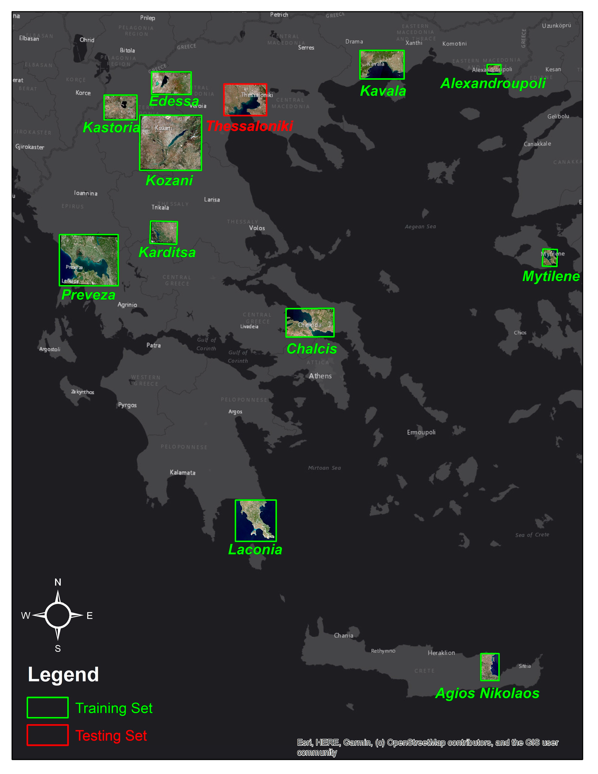
  • We create Sentinel-2 and Sentinel-1 composite images at 12 coastal, riparian or lakeside locations in Greece corresponding to specific time ranges within the year 2020. The resulting images, each containing 17 channels, along with associated land cover annotation from the ESA WorldCover product, will be freely provided as an open dataset for training DL models for land cover classification;
  • We use this dataset to train a modified U-TAE approach, which uses band attention instead of temporal attention;
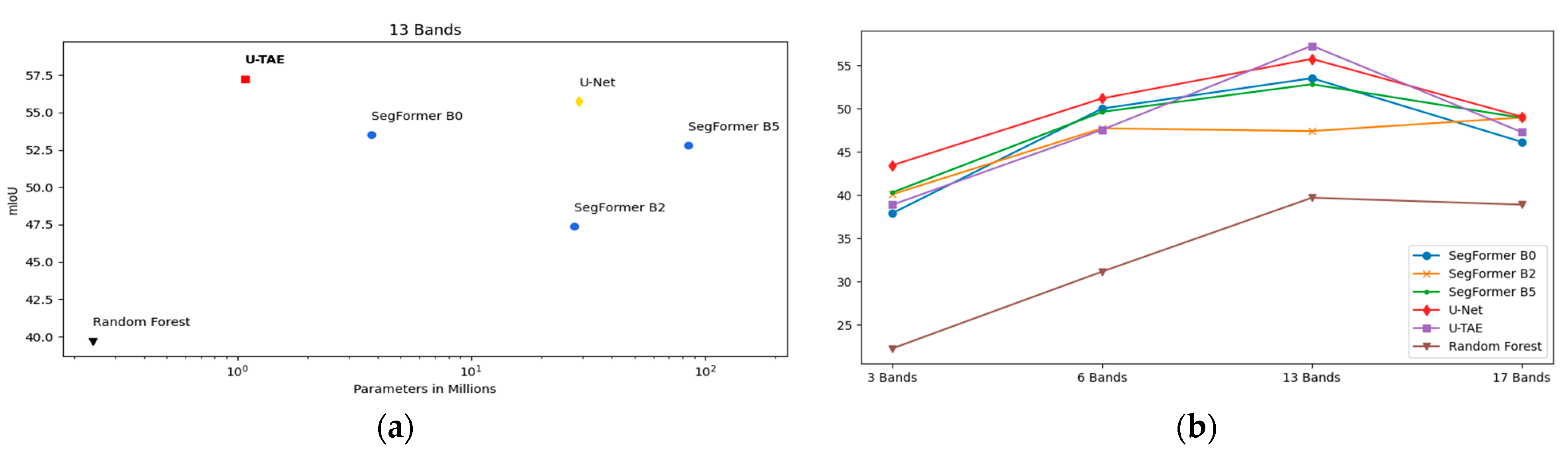
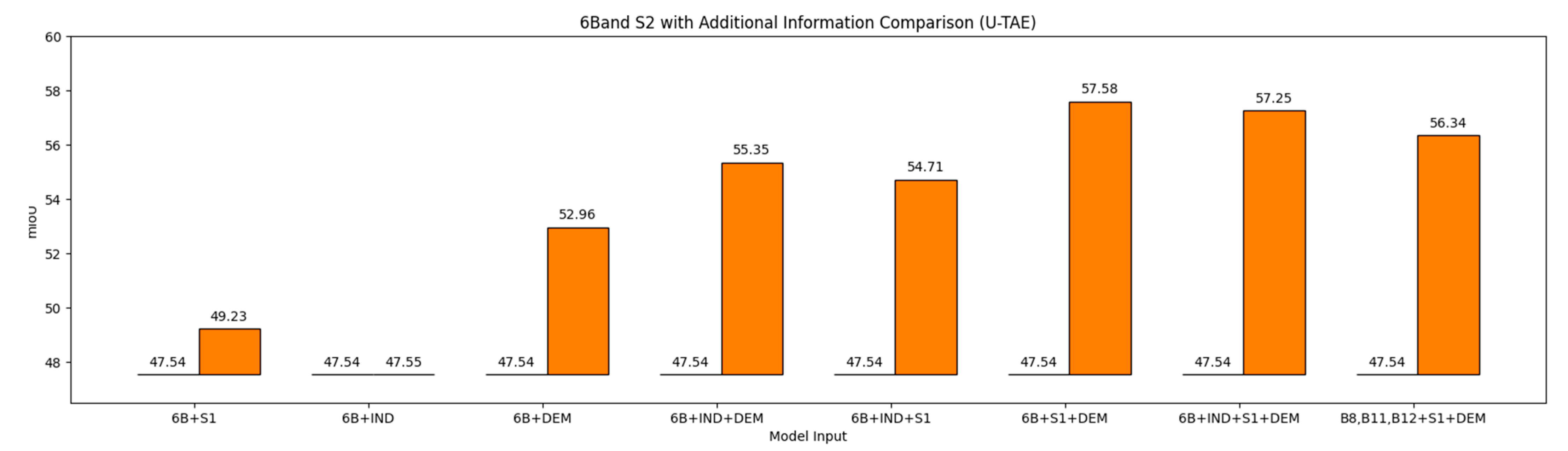
  • We evaluate the performance obtained by selecting as input different band combinations and;
  • We perform a comparative performance evaluation of the proposed approach with two state-of-the-art deep semantic segmentation (U-NET, SegFormer) architectures and one traditional ML algorithm (random forest).

2. Materials and Methods

2.1. Overview

An overview of the proposed approach is illustrated in Figure 1. More specifically, Sentinel-2 and Sentinel-1 composite images are created and pre-processed using Google Earth Engine from 12 coastal, riparian, or lakeside locations in Greece corresponding to specific time ranges within the year 2020. The resulting images are split into 256 × 256 tiles and associated labels are obtained from the ESA WorldCover product. Training of the different ML/DL approaches is performed using input data from 11 regions, while the last region is used for testing. The following subsections will describe in more detail this methodology.

2.2. Regions of Interest

From both a physical and anthropogenic geographical perspective, Greek landscapes represent three different, albeit highly variable and historically changing, geographical entities [42], namely (a) island, (b) coastal, and (c) inland landscapes. In order to create the training set, eleven region of interests (ROIs) were selected, namely three island cities (Chalcida in Euboea, Mytilene in Lesvos, and Agios Nikolaos in Crete), four coastal cities (Kavala, Alexandroupoli, Preveza, and Northeastern Laconia) and four lakeside or riparian inland regions (Edessa, Kastoria, Kozani, and Karditsa), as shown in Figure 2. The ROI used for testing is the greater region of Thessaloniki, which includes Thermaikos Gulf and the Axios Delta National Park. The area was chosen as the Greek pilot site for the EPIPELAGIC project [43], as it is a coastal area that contains three river deltas and has different land uses as well as various economic activities, which in many cases have significant environmental impacts.

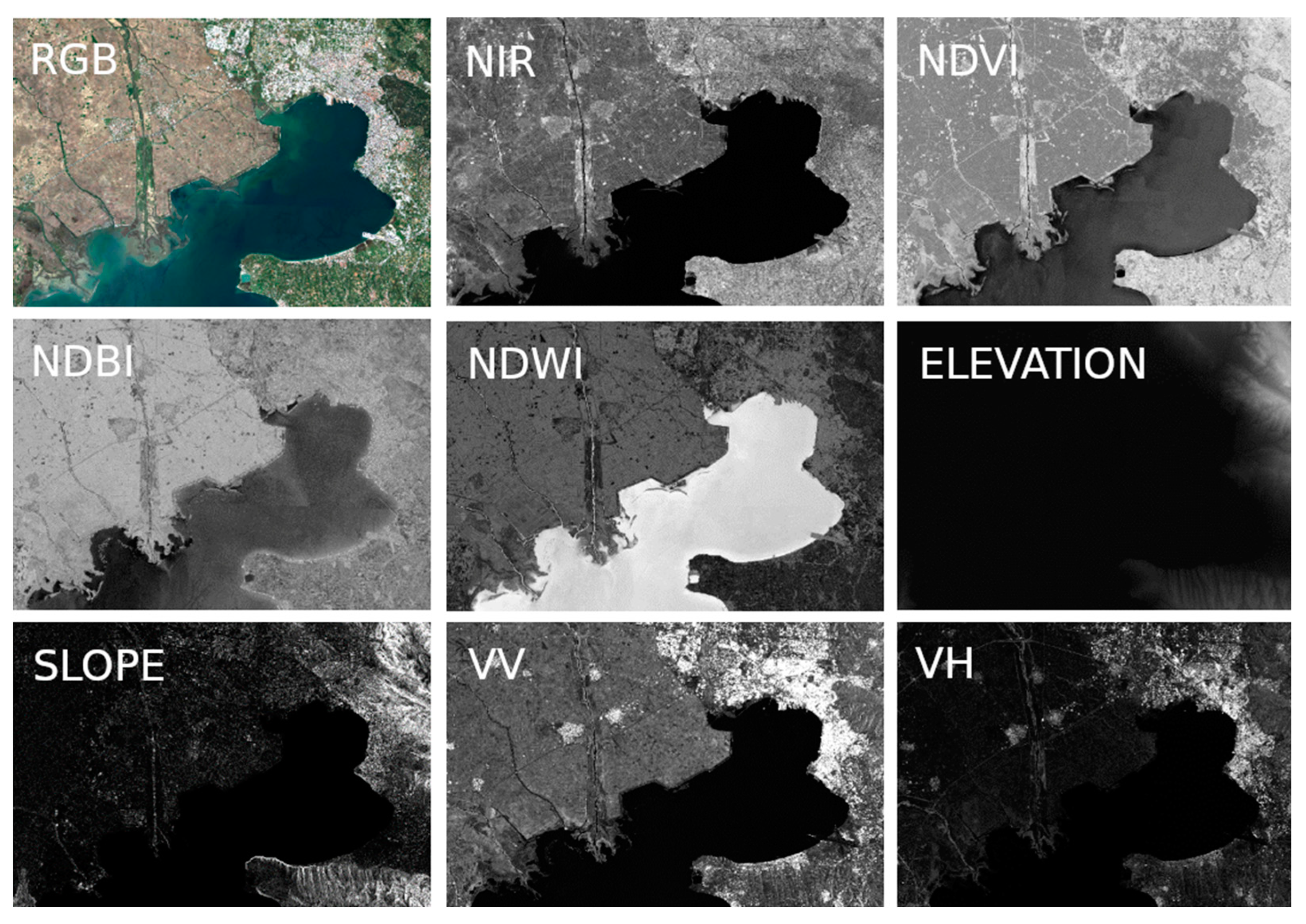
2.3. Remote Sensing Data Selection

We opt to use satellite data from Sentinel-2 (Level 2A) [3] and Sentinel-1 (GRD) [4] missions, within the year 2020 (two median six months images, January to June and July to December) as well as associated spectral indices and digital elevation model (DEM) products are used for the creation of the training and testing datasets. The corresponding annotations are obtained from the ESA WorldCover v100 project.
Specifically, we use Sentinel-2 Level-2A images with 12 multispectral bands (resolutions of 10, 20, and 60 m/pixel) representing surface reflectance. However, similarly to [38], the noisy atmospheric bands (i.e., bands for aerosols and water vapor with 60 m/pixel) are omitted since they cannot provide any useful information, as on all images, cloud masks are applied.
Additionally, the Sentinel-1 GRD (S1) data used are the backscatter intensities that can be measured from each of two polarization channels, namely VH and VV. The active microwave data from the synthetic aperture radar (SAR) has enormous potential for mapping and monitoring land cover, notably in identifying the water bodies and wetland vegetation [4]. This is due to the capabilities of day and night observation, as well as cloud penetration.
Furthermore, to improve the overall land cover classification, three indices derived from the Sentinel-2 mission were included: the normalised difference vegetation index (NDVI) [44], the normalised difference built-up index (NDBI) [45], and the normalised difference water index (NDWI) [46], which are calculated based on the Equations (1)–(3):
N D V I = N I R R E D N I R + R E D  
N D B I = S W I R 1 N I R S W I R 1 + N I R  
N D W I = G R E E N N I R G R E E N + N I R   .
NDVI provides important cues regarding the existence of live green vegetation. It is often used to monitor drought, forecast agricultural production, and assist in forecasting fire zones and desert offensive maps. NDBI distinguishes urban areas with higher reflectance in the shortwave infrared spectral range and therefore it is used to specify human settlements, as well as other infrastructure. Finally, high values of NDWI are used to identify water bodies.
Additionally, the 30 m resolution digital surface model (DSM) from the ALOS World 3D—30 m (AW3D30) v3.2 product released in 2021 from the Japan Aerospace Exploration Agency (JAXA) was selected to supply auxiliary data, namely elevation and slope, that can be useful for detecting land cover. Figure 3 illustrates different bands from the input data set used for testing.
The annotation data used for training and evaluation was obtained from the European Space Agency (ESA) WorldCover v100 v3.2 product [13], released in 2021. This product provides a global land cover map for the year 2020 at 10 m resolution based on Sentinel-1 and Sentinel-2 data. It consists of eleven land cover classes, namely trees, shrubland, grassland, cropland, built-up, barren/sparse vegetation, snow and ice, open water, herbaceous wetland, mangroves, and moss and lichen. Three classes (snow and ice, mangroves, and moss and lichen) are not present in the ROIs used for this study and were omitted. As shown in Figure 4, the dataset is greatly unbalanced, with more than half of the dataset belonging to two classes (trees and open water), while three classes (herbaceous wetland, built-up, and barren/sparse vegetation) are underrepresented (0.8%, 2.8%, and 3.1% of the dataset, respectively).

2.4. Remote Sensing Preprocessing

Google Earth Engine (GEE) is a platform for scientific analysis and visualisation of geospatial datasets. GEE also provides application programming interfaces (in JavaScript and Python) and other tools for the analysis of large datasets [41]. Pre-processing was performed remotely using Python in GEE, resulting in a single multichannel image for each ROI, which was then downloaded locally.
Specifically, regarding the Sentinel-2 Level 2A multispectral imagery, a two-step preprocessing procedure is used: first, all available images in the year 2020 with less than 5% cloud coverage are selected and any cloud and cirrus pixels are masked-out using the QA60 cloud mask. At the second stage, a temporal median filter is applied to each pixel of the selected images, resulting in a single, noise-free composite multispectral image. Similarly, regarding Sentinel-1 SAR GRD imagery, a temporal median filter is applied to each pixel of all available images in the year 2020, resulting in a single multichannel image composite. Finally, two additional channels are generated from the DSM band of the ALOS AW3D30 product, i.e., the elevation (ELEVATION) value in meters provided for each pixel, as well as the slope (SLOPE) in degrees, which was computed using a built-in GEE function. All bands and products were resampled to 10 m/pixel resolution to achieve the same resolution of the WorldCover product.

2.5. Land Cover Classification Algorithms

In the following, we briefly introduce our proposed modified version of U-TAE as well as two other popular semantic segmentation algorithms, namely the CNN-based U-Net and the transformer-based SegFromer. We also present the well-known random forest algorithm, which is often used for land cover classification. In more detail:
(a)
U-Net with temporal attention encoder (U-TAE) [40]: This model encodes a multitemporal image sequence in the following steps: (1) a shared multi-level spatial convolutional encoder embeds each image in a simultaneous and independent way, (2) a temporal attention encoder creates a single feature map for every level by stacking the temporal dimensions of the resulting sequence. Specifically, in order to reduce the memory and computational requirements, for every pixel it produces temporal attention masks at the lowest resolution, which are then spatially interpolated at all resolutions. (3) A convolutional decoder calculates features at every resolution level and the final predicted segmentation mask is produced as the output of the highest resolution level;
The architecture uses group normalisation with 4 groups. The input of the original network was modified by changing the shape of the image time sequence from T × C × H × W to C × 1 × H × W, with T the number of temporal instances, C the number of channels, and H × W the height and width of each image. The first two dimensions were permuted to take advantage of the attention module of the U-TAE architecture and to ensure channel-wise attention.
(b)
U-Net [25]: This is a U-shaped architecture with an encoder and a decoder that extends the fully convolutional networks segmentation for semantic segmentation [47]. Through a step-by-step downsampling operation, high-level features from the encoder are extracted, while the decoder gradually upsamples these features and combines the output with skip connections to return the feature map to the size of the input. The use of skip connections is important to enable feature reusability and stabilise training and convergence;
(c)
SegFormer [37]: This is a hierarchical transformer architecture that extends the segmentation transformer (SETR) proposed in [34]. In the encoding stage, efficient transformer modules are used, while in the decoding stage, multilayer perceptrons (MLPs) are applied. Specifically, a transformer encoder that has a hierarchical structure outputs multiple features, each divided by ascending powers of two without positional encoding. This increases performance even if the training and testing resolutions are different. A lightweight MLP decoder aggregates information from different layers, combining both local and global attention to produce powerful representations. Advantages of the proposed algorithm include: (i) the hierarchical transformer structure, which significantly reduces the computational cost without restricting the effective receptive field, (ii) the positional-encoding free encoder, and (iii) a simple, straightforward, and very efficient decoder;
(d)
The random forest (RF) algorithm [48] is an ensemble learning algorithm, i.e., combines multiple ML models to obtain the final solution to classification or regression problems. In this case, we used multiple decision trees for land cover classification. Decision tree-based classifiers were widely studied over the past two decades and were used in many practical applications, including remote sensing, due to several advantages: the concept is intuitively appealing, training is relatively simple, and classification is fast. Unlike many machine learning models that function as “black boxes”, a decision tree is an explainable machine learning algorithm and its logic can be fully understood by simply visualising the decision tree. Random forest algorithms for classification use a learning method that builds a set of decision trees during training and outputs the average prediction of the individual trees. Random decision forests are preferred because they avoid the tendency of decision trees to overfit on the training set. Although some degree of explainability is lost as the number of decision trees increases, it is still possible to determine feature importance in a trained RF model.

2.6. Implementation Details and Metrics
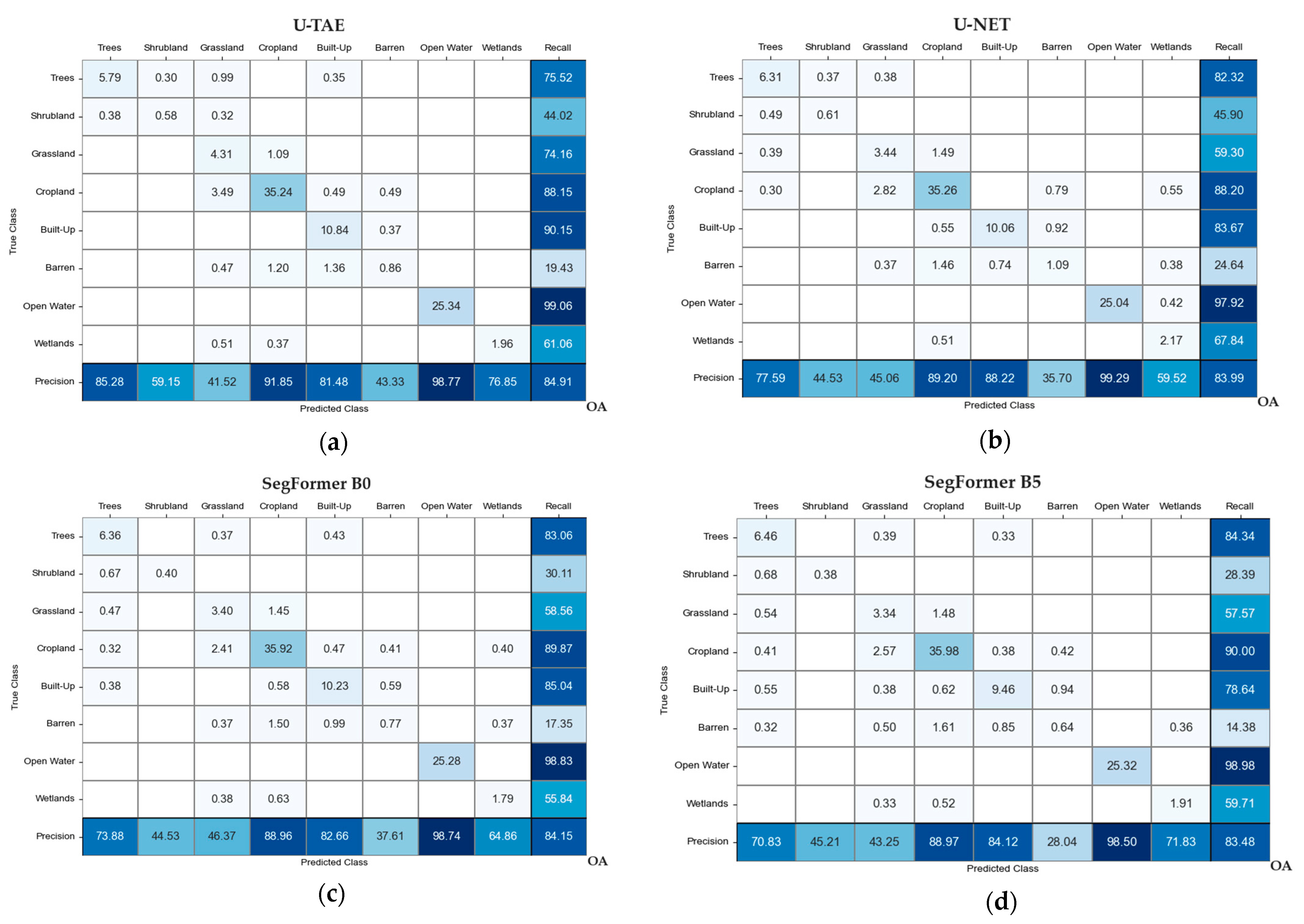
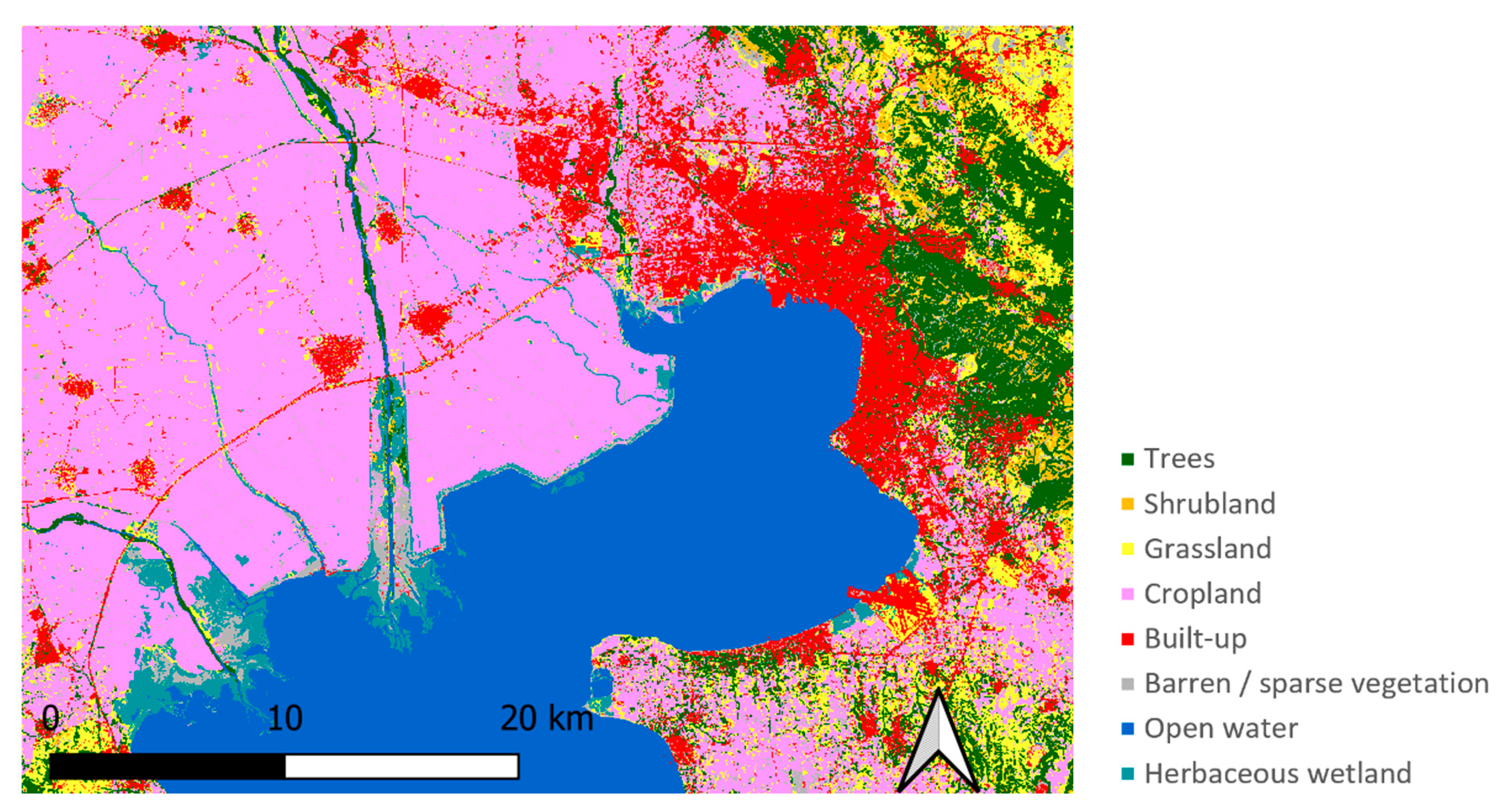
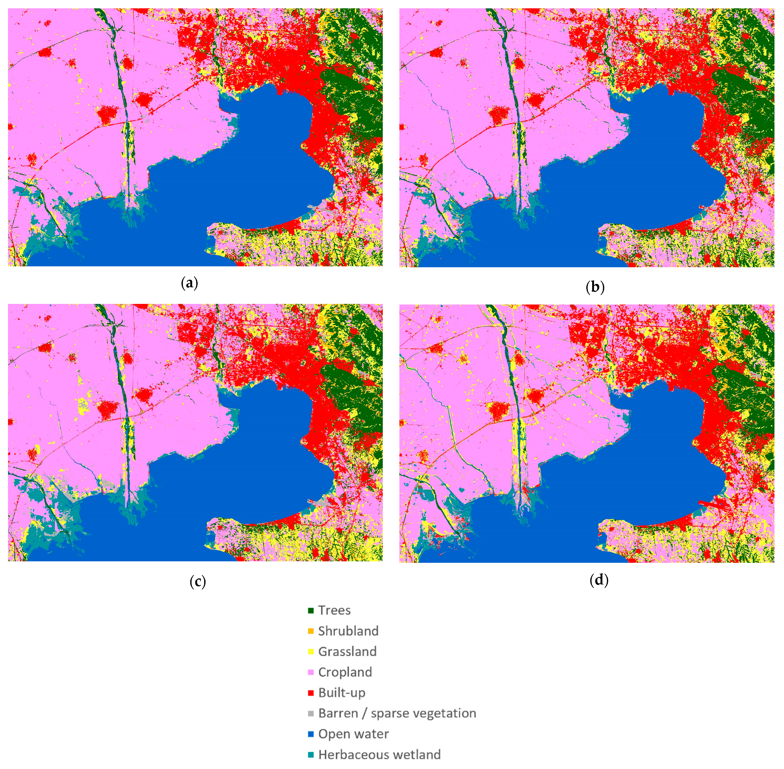
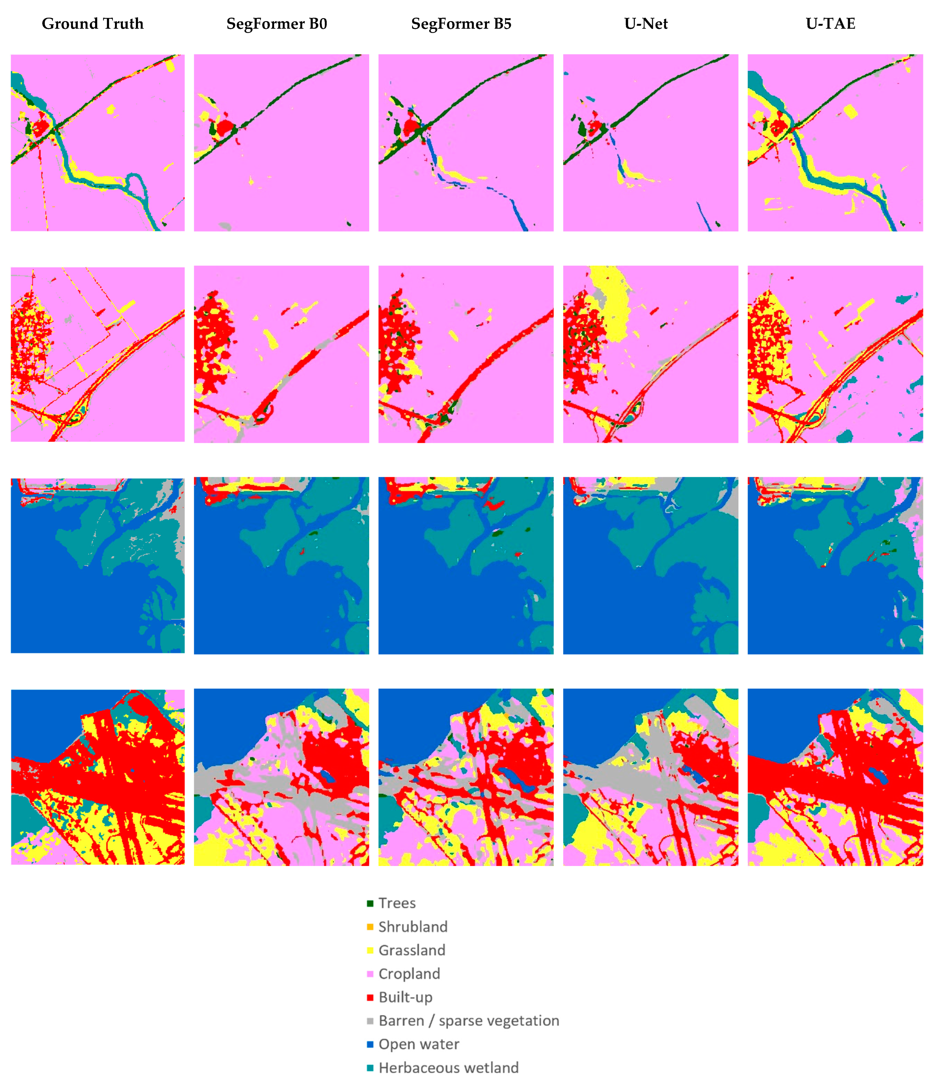
In the case of the three DL algorithms, the training process was implemented using PyTorch and was run on a NVIDIA RTX 3080 with 12 GB of memory. To overcome the memory constraints and requirements for images of fixed size, all training and testing images are split into non-overlapping square tiles of size 256 × 256. Thus, 4258 training and 204 square tiles were created and all DL algorithms were trained on all available tiles of size 256 × 256.
The U-TAE model was run using the official code repository, where the required changes to the model architecture were made to use channel attention instead of temporal attention. The initial learning rate value is 10−3, with an Adam optimiser and cross-entropy loss. Due to memory constraints, the U-TAE model was run using a batch size of 2, with the exception of the 17B combination, which used batch size of 1 (Table 1).
The SegFormer and the U-Net models were run using the mmsegmentation codebase [49], for efficient development and experimentation. The SegFormer models had a starting learning rate of 6 × 10⁻⁵, a polynomial learning rate schedule, and an AdamW optimizer [50]. The U-Net model used a SGD optimiser with a starting learning rate of 10−2. The batch size is 8 and cross-entropy loss for both models.
Data normalisation was performed on all deep learning algorithms by calculating (X-mean)/standard deviation, where X is the corresponding value, mean and standard deviation are concerning each corresponding image. This normalisation technique was seen to improve the accuracy of the results in preliminary tests that were omitted from the paper.
During training of the three deep learning models, no augmentation techniques were used. Furthermore, the U-Net and SegFormer models were adapted to accommodate multichannel image training, as the original techniques were developed for 3-channel RGB images.
Regarding the RF algorithm, in order to reduce the memory and computational requirements, a sampling grid is defined in all training images and only pixels on this sampling grid are considered for training. Experiments showed that the optimal grid cell size was equal to 64. The parameters of the random forest classifier were selected using the GridSearch function. For example, when using 17 bands, the optimal parameters are: (a) number of trees: 41, (b) minimum samples in order to split a tree: 10, and (c) minimum number of leaf samples on a leaf node: 2.
To evaluate the results of the algorithms, two metrics were used: overall accuracy (OA) and mean intersection-over-union (mIoU). In semantic segmentation tasks, mIoU is widely used as an evaluation metric. It is a measure of how well the predicted segmentation map aligns with the ground truth segmentation map. Another important metric in every classification task is overall accuracy (OA). OA is the ratio of the correctly classified samples to the total number of samples, as shown in Equation (4). More specifically:
O A = T P + T N T P + T N + F P + F N
where TP (FP) is the number of true (false) positives and TN (FN) is the number of true (false) negatives. On the other hand, mIoU is defined as the average of the intersection-over-union (IoU) values between each predicted class and ground truth class across all pixels in an image, i.e.,
m I o U = 1 C 1 C I o U C
where C is the total number of classes and IoU:
I o U = T P T P + F P + F N   .  

3. Results

3.1. Experimental Results

In the experiments, we use different band combinations as input. For more clarity, in Table 1, we provide a dictionary of codes describing each band combination used.
The experimental results for the models are presented in Table 2. The highest mIoU and OA values were obtained using the U-TAE and U-Net models with the 13B combination, while the SegFormer model and its variations demonstrate generally inferior performance.
The U-TAE model yields better results than the other two DL models, with much fewer parameters. In Figure 5a we can see that with 13 band input the U-TAE model both outperforms the other two in mIoU score, and is lighter in parameters. In Figure 5b, the chart shows the mIoU scores of Table 2, where U-TAE is clearly outperforming the other models.
It is also noteworthy that increasing the input bands from 13 to 17 actually decreases the score. That means that not all the information in the input is beneficial to the accuracy of the model, and the addition of certain bands can actually reduce it. All models show a decline in the metrics when moving from Sentinel-2 6 bands to 10 bands, suggesting that more is not always better. In the following ablation study, we will try to further investigate this phenomenon.
Aside from the metrics, it is important that the model also has good recall, precision, and overall more concise class predictions. In Figure 6a–d we see that the U-TAE model has the best recall and precision compared to the other models. Additionally, the U-TAE model predicts the classes with less representation in the dataset, i.e., barren/sparse vegetation, built-up, and herbaceous wetland, with fewer misclassifications, i.e., FPs and FNs.
Figure 7 and Figure 8 illustrate the ground truth segmentation map of the testing set (Thessaloniki), and the predicted segmentation maps of each model for 13B. From the generated maps we can see that the U-TAE model is able to capture the minute intricacies of the area better than the other models. For instance, the SegFormer and U-Net models cannot classify the small grassland regions in the upper left part of the map as well as the U-TAE model. We can also observe that the U-TAE model is better at mapping the built-up class, thus representing the urban regions of the area more accurately. Figure 9 illustrates qualitative prediction results for selected regions of the testing dataset, clearly demonstrating the superior performance of the U-TAE model.

3.2. Band Combination Ablation Study

We conducted a study on the effects of using different band combinations as input to the modified U-TAE model, which achieved the highest mIoU (57.25%). The purpose of this study is to assess the importance of each band in real-world applications and to determine the band combinations that yield optimal results, avoiding use of unnecessary noisy information.
The combination of the 6B (from S2), S1, and DEM bands appeared to be the most successful input to the U-TAE model (mIoU: 57.58%), surpassing even the previous highest mIoU, which used additionally the IND bands. From Figure 10, it can be inferred that the addition of IND bands generally tends to confuse or hinder the model accuracy. On the contrary, the addition of DEM information seems to significantly improve results, indicating that the model benefits by the knowledge of the geographical terrain.
We also experimented with the 6B combination to examine the relative importance of RGB bands. Specifically, we used only the three thermal infrared S2 bands (NIR, SWIR1, and SWIR2), combined with the S1 and DEM bands. This configuration yields a result that is significantly higher than many other combinations (Figure 10) of information we examined, with a mIoU score that is close to the two highest. Thus, we observe that the infrared information is at least as important as the RGB, if not more, given that the mIoU decreases by only 1.24% when omitting the RGB bands.

4. Discussion

Recently, the utilisation of deep learning approaches using input from remote sensing images for land cover and land use classification gained popularity [51], as it can overcome limitations of already available products [52]. In this paper, we utilise a modified version of a robust semantic segmentation approach based on temporal attention, namely U-TAE, for land cover classification. We evaluate its performance by combining different remote sensing data and compare results against two other deep learning approaches, namely U-Net and SegFormer, as well as a traditional ML method, RF.
The use of deep learning for land cover classification by fusing multispectral and SAR data started in early studies [53], where both Sentinel-1 as well as Landsat 8 data are used; Ref. [54] implemented a U-Net network for large-scale land cover classification using only RGB Sentinel-2 images and hand-labeled annotation, achieving promising results. In [55], a dataset containing 27,000 labeled and geo-referenced images is constructed for land use and land cover classification, while a correspondng benchmark based on CNNs is also provided. In [56], a large-scale project is presented, exploiting cloud-based systems and using ML for land cover classification.
While some studies suggested that the NDVI and the NIR band are the most important bands for land cover classification considering vegetation [57], we also recommend incorporating Sentinel-1 data, as they enhance the ability to identify vegetation. This conclusion is supported both by our results as well as by the results of [58], which demonstrate the benefits of fusing Sentinel-2 and Sentinel-1 data. Another study, Ref. [59] highlighted that ML algorithms may outperform conventional DL algorithms when large datasets are not available.
Recently, transformer-based approaches were also widely used for land cover and crop classification with Sentinel 2 imagery [38,60,61,62,63], but mainly employ temporal attention. Scheibenreif et al. [64] used large datasets of unlabelled remote sensing data (Sentinel-2 and Sentinel-1 image pairs) for self-supervised pre-training of vision transformers. Such self-supervised transformer-based methods can offer great potential; as the labeling of large remote sensing datasets is a very tedious procedure, such self-supervised approaches have strong potential.
We believe that in the near future, transformer-based architectures, which employ self-attention to differentially weigh parts of the input signal based on their significance, will play a crucial role in advancing remote sensing land cover classification. Transformers already demonstrated impressive results in numerous ML applications, although in certain cases, CNNs may still outperform them. Additionally, transformer models are highly parallelizable, and thus suitable for processing large datasets in a reasonable time frame.
Some limitations of the proposed approach include the fact that temporal attention is actually replaced by band attention, while a combination of both could provide improved results. Furthermore, any errors in the WorldCover product (or other similar products in the future) that are used as ground truth will inevitably be propagated in our proposed approach. Finally, another challenge is the dynamic nature of some land cover classes, such as agriculture, wetlands, etc., which are often changing from time to time. This makes it more difficult to accurately determine land cover, when a longer time frame is used.

5. Conclusions

The results of this paper indicate that deep learning (DL) algorithms demonstrate significantly superior performance against traditional machine learning (ML) algorithms in the land cover classification field. It is also noteworthy that all algorithms demonstrate similar behaviour for specific band combinations, with the best performance obtained by the 13B combination. This suggests that the information contained within these bands is critical for accurate classification. This assumption is justified by the provided ablation study, where we highlighted the importance of S1 (VV and VH bands) as well as DEM (ELEVATION and SLOPE bands), which were seen to significantly affect the algorithm performance. Furthermore, the NIR, SWIR1, and SWIR2 Sentinel-2 bands seem to offer important information, as they result in good performance even without the addition of RGB bands. Furthermore, the modification of the U-TAE algorithm to provide channel (instead of temporal) attention seems to be promising for land cover classification. The U-TAE algorithm’s efficiency and simplicity, with the least amount of parameters compared to other DL algorithms, makes it an appealing choice. This is a significant outcome, as it highlights U-TAE’s potential to outperform not only conventional DL algorithms, such as U-Net, but also advanced hierarchical transformer-based algorithms, such as SegFormer. Based on the results obtained in this study, future work will involve the classification of 3-month image composites using the U-TAE. Furthermore, we plan to use similar approaches to directly assess land cover changes through time. This approach could provide valuable insights into land use changes and their potential impact on the environment, enabling more effective strategies for land management.
Finally, we need to note that all land cover classification approaches examined in this paper, including U-TAE, are actually pixel-based. Extensions towards object-based (or “panoptic” in ML terminology) segmentation were already proposed [40]. This is an interesting future direction, but also more challenging, as the shape of the land cover “objects” is arbitrary, and is expected to have higher complexity.

Author Contributions

Conceptualization, N.G. and A.T.; methodology, A.T. and N.G.; software, K.M. and A.T.; validation, N.G.; formal analysis, A.T., K.M. and N.G.; investigation, N.G.; resources, N.G.; data curation, A.T.; writing—original draft preparation, A.T.; writing—review and editing, A.T., K.M. and N.G.; visualization, A.T.; supervision, N.G.; project administration, N.G. All authors have read and agreed to the published version of the manuscript.

Funding

This research was funded by European Union and Greece, grant number T7ΔΚI-00160 & ΚΜΡ6-0079153.

Data Availability Statement

The created dataset will be freely provided if the manuscript is accepted.

Acknowledgments

This research was co-financed by the European Regional Development Fund of the European Union and Greek national funds through (a) the Operational Program Competitiveness, Entrepreneurship and Innovation, under the call RESEARCH–CREATE–INNOVATE (project code: T7ΔΚI-00160—“ExPert Integrated support system for CoastaL mixed urbAn–industrial—critical infrastructure monitoring using Combined technologies—EPIPELAGIC”), and (b) under the framework of the Action «Investment Plans of Innovation» of the Operational Program «Central Macedonia 2014 2020» as part of the project «INFOROAD—Development of an innovative online tool for mapping and monitoring the forest and rural road network» (Project code: ΚΜΡ6-0079153).

Conflicts of Interest

The authors declare no conflict of interest.

References

  1. Kaplan, G.; Avdan, U. Sentinel-1 and sentinel-2 data fusion for wetlands mapping: Balikdami, turkey. Int. Arch. Photogramm. Remote Sens. Spat. Inf. Sci. 2018, 42, 729–734. [Google Scholar] [CrossRef] [Green Version]
  2. Solórzano, J.V.; Mas, J.F.; Gao, Y.; Gallardo-Cruz, J.A. Land Use Land Cover Classification with U-Net: Advantages of Combining Sentinel-1 and Sentinel-2 Imagery. Remote Sens. 2021, 13, 3600. [Google Scholar] [CrossRef]
  3. Drusch, M.; Del Bello, U.; Carlier, S.; Colin, O.; Fernandez, V.; Gascon, F.; Hoersch, B.; Isola, C.; Laberinti, P.; Martimort, P.; et al. Sentinel-2: ESA’s optical high-resolution mission for GMES operational services. Remote Sens. Environ. 2012, 120, 25–36. [Google Scholar] [CrossRef]
  4. Torres, R.; Snoeij, P.; Geudtner, D.; Bibby, D.; Davidson, M.; Attema, E.; Potin, P.; Rommen, B.; Floury, N.; Brown, M.; et al. GMES Sentinel-1 mission. Remote Sens. Environ. 2012, 120, 9–24. [Google Scholar] [CrossRef]
  5. Roy, D.P.; Wulder, M.A.; Loveland, T.R.; Woodcock, C.E.; Allen, R.G.; Anderson, M.C.; Helder, D.; Irons, J.R.; Johnson, D.M.; Kennedy, R.; et al. Landsat-8: Science and product vision for terrestrial global change research. Remote Sens. Environ. 2014, 145, 154–172. [Google Scholar] [CrossRef] [Green Version]
  6. Cornelia, A.M. Advantages of Identifying Urban Footprint using Sentinel-1. In Proceedings of the FIG Congress 2018 Embracing Our Smart World Where the Continents Connect: Enhancing the Geospatial Maturity of Societies, Istanbul, Turkey, 6–11 May 2018. [Google Scholar]
  7. Tzouvaras, M.; Kouhartsiouk, D.; Agapiou, A.; Danezis, C.; Hadjimitsis, D.G. The use of Sentinel-1 synthetic aperture radar (SAR) images and open-source software for cultural heritage: An example from Paphos area in Cyprus for mapping landscape changes after a 5.6 magnitude earthquake. Remote Sens. 2019, 11, 1766. [Google Scholar] [CrossRef] [Green Version]
  8. McCarthy, M.J.; Colna, K.E.; El-Mezayen, M.M.; Laureano-Rosario, A.E.; Méndez-Lázaro, P.; Otis, D.B.; Toro-Farmer, G.; Vega-Rodriguez, M.; Muller-Karger, F.E. Satellite remote sensing for coastal management: A review of successful applications. Environ. Manag. 2017, 60, 323–339. [Google Scholar] [CrossRef]
  9. Nayak, S. Coastal zone management in India− present status and future needs. Geo-Spat. Inf. Sci. 2017, 20, 174–183. [Google Scholar] [CrossRef]
  10. Faruque, J.; Vekerdy, Z.; Hasan, Y.; Islam, K.Z.; Young, B.; Ahmed, M.T.; Monir, M.U.; Shovon, S.M.; Kakon, J.F.; Kundu, P. Monitoring of land use and land cover changes by using remote sensing and GIS techniques at human-induced mangrove forests areas in Bangladesh. Remote Sens. Appl. Soc. Environ. 2022, 25, 100699. [Google Scholar] [CrossRef]
  11. Rakhlin, A.; Davydow, A.; Nikolenko, S. Land cover classification from satellite imagery with u-net and lovász-softmax loss. In Proceedings of the IEEE Conference on Computer Vision and Pattern Recognition Workshops, Salt Lake City, UT, USA, 18–22 June 2018; pp. 262–266. [Google Scholar]
  12. Bossard, M.; Feranec, J.; Otahel, J. CORINE Land Cover Technical Guide: Addendum; European Environment Agency: Copenhagen, Denmark, 2000; Volume 40.
  13. Zanaga, D.; Van De Kerchove, R.; De Keersmaecker, W.; Souverijns, N.; Brockmann, C.; Quast, R.; Wevers, J.; Grosu, A.; Paccini, A.; Vergnaud, S.; et al. ESA WorldCover 10 m 2020 v100; OpenAIRE: Los Angeles, CA, USA, 2021. [Google Scholar] [CrossRef]
  14. Jordi, I.; Marcela, A.; Benjamin, T.; Olivier, H.; Silvia, V.; David, M.; Gerard, D.; Guada-lupe, S.; Sophie, B.; Pierre, D.; et al. Assessment of an operational system for crop type map production using high temporal and spatial resolution satellite optical imagery. Remote Sens. 2015, 7, 12356–12379. [Google Scholar]
  15. Pelletier, C.; Valero, S.; Inglada, J.; Champion, N.; Dedieu, G. Assessing the robustness of Random Forests to map land cover with high resolution satellite image time series over large areas. Remote Sens. Environ. 2016, 187, 156–168. [Google Scholar] [CrossRef]
  16. Siachalou, S.; Tsakiri-Strati, M. A hidden Markov models approach for crop classification: Linking crop phenology to time series of multi-sensor remote sensing data. Remote Sens. 2015, 7, 3633–3650. [Google Scholar] [CrossRef] [Green Version]
  17. Giordano, S.; Bailly, S.; Landrieu, L.; Chehata, N. Improved crop classification with rotation knowledge using Sentinel-1 and -2 time series. Photogramm. Eng. Remote Sens. 2020, 86, 431–441. [Google Scholar] [CrossRef]
  18. Devadas, R.; Denham, R.J.; Pringle, M. Support vector machine classification of object-based data for crop map-ping, using multi-temporal landsat imagery. International archives of the photogrammetry. Remote Sens. Spat. Inf. Sci. 2012, 39, 185–190. [Google Scholar]
  19. Hu, Q.; Wu, W.-B.; Song, Q.; Lu, M.; Chen, D.; Yu, Q.-Y.; Tang, H.-J. How do temporal and spectral features matter in crop classification in Heilongjiang Province, China? J. Integr. Agric. 2017, 16, 324–336. [Google Scholar] [CrossRef]
  20. Nguyen, L.H.; Joshi, D.R.; Clay, D.E.; Henebry, G.M. Characterizing land cover/land use from multiple years of Landsat and MODIS time series: A novel approach using land surface phenology modeling and ran-dom forest classifier. Remote Sens. Environ. 2020, 238, 111017. [Google Scholar] [CrossRef]
  21. Waldrop, M.M. The chips are down for Moore’s law. Nat. News 2016, 530, 144. [Google Scholar] [CrossRef] [PubMed] [Green Version]
  22. Alem, A.; Kumar, S. Deep learning methods for land cover and land use classification in remote sensing: A review. In Proceedings of the 2020 8th International Conference on Reliability, Infocom Technologies and Optimization (Trends and Future Directions)(ICRITO), Noida, India, 4–5 June 2020; IEEE: Piscataway, NJ, USA, 2020; pp. 903–908. [Google Scholar]
  23. Seydi, S.; Hasanlou, M.; Amani, M. A new end-to-end multi-dimensional CNN framework for land cover/land use change detection in multi-source remote sensing datasets. Remote Sens. 2020, 12, 2010. [Google Scholar] [CrossRef]
  24. Camalan, S.; Cui, K.; Pauca, V.P.; Alqahtani, S.; Silman, M.; Chan, R.; Plemmons, R.J.; Dethier, E.N.; Fernandez, L.E.; Lutz, D.A. Change detection of amazonian alluvial gold mining using deep learning and sentinel-2 imagery. Remote Sens. 2022, 14, 1746. [Google Scholar] [CrossRef]
  25. Ronneberger, O.; Fischer, P.; Brox, T. U-net: Convolutional networks for biomedical image segmentation. In Proceedings of the International Conference on Medical Image Computing and Computer-Assisted Intervention, Munich, Germany, 5–9 October 2015; Springer: Cham, Germany, 2015; pp. 234–241. [Google Scholar]
  26. Mohajerani, S.; Saeedi, P. Cloud-Net: An end-to-end cloud detection algorithm for Landsat 8 imagery. In Proceedings of the IGARSS 2019–2019 IEEE International Geoscience and Remote Sensing Symposium, Yokohama, Japan, 28 July–2 August 2019; IEEE: Piscataway, NJ, USA, 2019; pp. 1029–1032. [Google Scholar]
  27. Ye, H.; Liu, S.; Jin, K.; Cheng, H. CT-UNet: An Improved Neural Network Based on U-Net for Building Segmenta-tion in Remote Sensing Images. In Proceedings of the 2020 25th International Conference on Pattern Recognition (ICPR), Milan, Italy, 10–15 January 2021; pp. 166–172. [Google Scholar] [CrossRef]
  28. He, N.; Fang, L.; Plaza, A. Hybrid first and second order attention Unet for building segmentation in re-mote sensing images. Sci. China Inf. Sci. 2020, 63, 140305. [Google Scholar] [CrossRef] [Green Version]
  29. Jiao, L.; Huo, L.; Hu, C.; Tang, P. Refined UNet: UNet-based refinement network for cloud and shadow precise segmentation. Remote Sens. 2020, 12, 2001. [Google Scholar] [CrossRef]
  30. Hou, Y.; Liu, Z.; Zhang, T.; Li, Y. C-Unet: Complement UNet for remote sensing road extraction. Sensors 2021, 21, 2153. [Google Scholar] [CrossRef]
  31. Vaswani, A.; Shazeer, N.; Parmar, N.; Uszkoreit, J.; Jones, L.; Gomez, A.N.; Kaiser, Ł.; Polosukhin, I. Attention Is All You Need. arXiv e-prints 2017, arXiv:1706.03762. [Google Scholar]
  32. Aleissaee, A.A.; Kumar, A.; Anwer, R.M.; Khan, S.; Cholakkal, H.; Xia, G.-S.; Khan, F.S. Transformers in remote sensing: A survey. Remote Sens. 2022, 15, 1860. [Google Scholar] [CrossRef]
  33. Dosovitskiy, A.; Beyer, L.; Kolesnikov, A.; Weissenborn, D.; Zhai, X.; Unterthiner, T.; Dehghani, M.; Minderer, M.; Heigold, G.; Gelly, S.; et al. An image is worth 16×16 words: Transformers for image recognition at scale. arXiv 2020, arXiv:2010.11929. [Google Scholar]
  34. Zheng, S.; Lu, J.; Zhao, H.; Zhu, X.; Luo, Z.; Wang, Y.; Fu, Y.; Feng, J.; Xiang, T.; Torr, P.H.; et al. Rethinking semantic segmentation from a sequence-to-sequence perspective with transformers. In Proceedings of the IEEE/CVF Conference on Computer Vision and Pattern Recognition, Nashville, TN, USA, 20–25 June 2021; pp. 6881–6890. [Google Scholar]
  35. Wang, W.; Xie, E.; Li, X.; Fan, D.-P.; Song, K.; Liang, D.; Lu, T.; Luo, P.; Shao, L. Pyramid vision transformer: A versatile backbone for dense prediction without convolutions. In Proceedings of the IEEE/CVF International Conference on Computer Vision, Montreal, QC, Canada, 10–17 October 2021; pp. 568–578. [Google Scholar]
  36. Liu, Z.; Lin, Y.; Cao, Y.; Hu, H.; Wei, Y.; Zhang, Z.; Lin, S.; Guo, B. Swin transformer: Hierarchical vision transformer using shifted windows. In Proceedings of the IEEE/CVF International Conference on Computer Vision, Montreal, QC, Canada, 10–17 October 202; pp. 10012–10022.
  37. Xie, E.; Wang, W.; Yu, Z.; Anandkumar, A.; Alvarez, J.M.; Luo, P. SegFormer: Simple and efficient design for semantic segmentation with transformers. Adv. Neural Inf. Process. Syst. 2021, 34, 12077–12090. [Google Scholar]
  38. Garnot, V.S.F.; Landrieu, L.; Giordano, S.; Chehata, N. Satellite image time series classification with pixel-set encoders and temporal self-attention. In Proceedings of the IEEE/CVF Conference on Computer Vision and Pattern Recognition, Seattle, WA, USA, 13–19 June 2020; pp. 12325–12334. [Google Scholar]
  39. Garnot, V.S.F.; Landrieu, L. Lightweight temporal self-attention for classifying satellite images time series. In Proceedings of the Advanced Analytics and Learning on Temporal Data: 5th ECML PKDD Workshop, AALTD 2020, Ghent, Belgium, 18 September 2020; Revised Selected Papers 6. Springer International Publishing: Berlin/Heidelberg, Germany, 2020; pp. 171–181. [Google Scholar]
  40. Garnot, V.S.F.; Landrieu, L. Panoptic segmentation of satellite image time series with convolutional temporal attention networks. In Proceedings of the IEEE/CVF International Conference on Computer Vision, Montreal, QC, Canada, 10–17 October 2021; pp. 4872–4881. [Google Scholar]
  41. Gorelick, N. Google earth engine. In EGU General Assembly Conference Abstracts; American Geophysical Union: Vienna, Austria, 2013; Volume 15, p. 11997. [Google Scholar]
  42. Terkenli, T.S. Landscape research in Greece: An overview. Belgeo. Rev. Belg. Géographie 2004, 2–3, 277–288. [Google Scholar] [CrossRef] [Green Version]
  43. Tzepkenlis, A.; Grammalidis, N.; Kontopoulos, C.; Charalampopoulou, V.; Kitsiou, D.; Pataki, Z.; Patera, A.; Nitis, T. An Integrated Monitoring System for Coastal and Riparian Areas Based on Remote Sensing and Machine Learning. J. Mar. Sci. Eng. 2022, 10, 1322. [Google Scholar] [CrossRef]
  44. DeFries, R.S.; Townshend, J.R.G. NDVI-derived land cover classifications at a global scale. Int. J. Remote Sens. 1994, 15, 3567–3586. [Google Scholar] [CrossRef]
  45. Zha, Y.; Gao, J.; Ni, S. Use of normalized difference built-up index in automatically mapping urban areas from TM imagery. Int. J. Remote Sens. 2003, 24, 583–594. [Google Scholar] [CrossRef]
  46. McFeeters, S.K. The use of the Normalized Difference Water Index (NDWI) in the delineation of open water features. Int. J. Remote Sens. 1996, 17, 1425–1432. [Google Scholar] [CrossRef]
  47. Long, J.; Shelhamer, E.; Darrell, T. Fully convolutional networks for semantic segmentation. In Proceedings of the IEEE Conference on Computer Vision and Pattern Recognition, Boston, MA, USA, 7–12 June 2015; pp. 3431–3440. [Google Scholar]
  48. L Breiman, L. Random Forests. Mach. Learn. 2001, 45, 5–32. [Google Scholar] [CrossRef] [Green Version]
  49. Contributors, MMSegmentation. OpenMMLab Semantic Segmentation Toolbox and Benchmark. 2020. Available online: https://github.com/open-mmlab/mmsegmentation (accessed on 7 April 2023).
  50. Loshchilov, I.; Hutter, F. Decoupled weight decay regularization. arXiv 2017, arXiv:1711.05101. [Google Scholar]
  51. Digra, M.; Dhir, R.; Sharma, N. Land use land cover classification of remote sensing images based on the deep learning approaches: A statistical analysis and review. Arab. J. Geosci. 2022, 15, 1003. [Google Scholar] [CrossRef]
  52. Malenovský, Z.; Rott, H.; Cihlar, J.; Schaepman, M.E.; García-Santos, G.; Fernandes, R.; Berger, M. Sentinels for science: Potential of Sentinel-1, -2, and -3 missions for scientific observations of ocean, cryosphere, and land. Remote Sens. Environ. 2012, 120, 91–101. [Google Scholar] [CrossRef]
  53. Kussul, N.; Lavreniuk, M.; Skakun, S.; Shelestov, A. Deep learning classification of land cover and crop types using remote sensing data. IEEE Geosci. Remote Sens. Lett. 2017, 14, 778–782. [Google Scholar] [CrossRef]
  54. Karra, K.; Kontgis, C.; Statman-Weil, Z.; Mazzariello, J.C.; Mathis, M.; Brumby, S.P. Global land use/land cover with Sentinel 2 and deep learning. In Proceedings of the 2021 IEEE International Geoscience and Remote Sensing Symposium IGARSS, Brussels, Belgium, 11–16 July 2021; IEEE: Piscataway, NJ, USA, 2021; pp. 4704–4707. [Google Scholar]
  55. Helber, P.; Bischke, B.; Dengel, A.; Borth, D. Eurosat: A novel dataset and deep learning benchmark for land use and land cover classification. IEEE J. Sel. Top. Appl. Earth Obs. Remote Sens. 2019, 12, 2217–2226. [Google Scholar] [CrossRef] [Green Version]
  56. Verde, N.; Kokkoris, I.P.; Georgiadis, C.; Kaimaris, D.; Dimopoulos, P.; Mitsopoulos, I.; Mallinis, G. National scale land cover classification for ecosystem services mapping and assessment, using multitemporal copernicus EO data and google earth engine. Remote Sens. 2020, 12, 3303. [Google Scholar] [CrossRef]
  57. Campos-Taberner, M.; García-Haro, F.J.; Martínez, B.; Izquierdo-Verdiguier, E.; Atzberger, C.; Camps-Valls, G.; Gilabert, M.A. Understanding deep learning in land use classification based on Sentinel-2 time series. Sci. Rep. 2020, 10, 17188. [Google Scholar] [CrossRef]
  58. Ienco, D.; Interdonato, R.; Gaetano, R.; Minh, D.H.T. Combining Sentinel-1 and Sentinel-2 Satellite Image Time Series for land cover mapping via a multi-source deep learning architecture. ISPRS J. Photogramm. Remote Sens. 2019, 158, 11–22. [Google Scholar] [CrossRef]
  59. Abdi, A.M. Land cover and land use classification performance of machine learning algorithms in a boreal landscape using Sentinel-2 data. GIScience Remote Sens. 2020, 57, 1–20. [Google Scholar] [CrossRef] [Green Version]
  60. Rußwurm, M.; Körner, M. Self-attention for raw optical satellite time series classification. ISPRS J. Photogramm. Remote Sens. 2020, 169, 421–435. [Google Scholar] [CrossRef]
  61. Stergioulas, A.; Dimitropoulos, K.; Grammalidis, N. Crop classification from satellite image sequences using a two-stream network with temporal self-attention. In Proceedings of the 2022 IEEE International Conference on Imaging Systems and Techniques (IST), Kaohsiung, Taiwan, 21–23 June 2022; IEEE: Piscataway, NJ, USA, 2022; pp. 1–6. [Google Scholar]
  62. Yuan, Y.; Lin, L. Self-supervised pretraining of transformers for satellite image time series classification. IEEE J. Sel. Top. Appl. Earth Obs. Remote Sens. 2020, 14, 474–487. [Google Scholar] [CrossRef]
  63. Martini, M.; Mazzia, V.; Khaliq, A.; Chiaberge, M. Domain-adversarial training of self-attention-based networks for land cover classification using multi-temporal Sentinel-2 satellite imagery. Remote Sens. 2021, 13, 2564. [Google Scholar] [CrossRef]
  64. Scheibenreif, L.; Hanna, J.; Mommert, M.; Borth, D. Self-supervised vision transformers for land-cover segmentation and classification. In Proceedings of the IEEE/CVF Conference on Computer Vision and Pattern Recognition, New Orleans, LA, USA, 18–24 June 2022; pp. 1422–1431. [Google Scholar]
Figure 1. Flowchart of the proposed land cover classification approach.
Remotesensing 15 02027 g001
Figure 2. The selected training sites (green polygon) as well as the testing site (red polygon).
Remotesensing 15 02027 g002
Figure 3. Visualisation of different bands from the input dataset.
Remotesensing 15 02027 g003
Figure 4. Bar chart showing the distribution of the eight classes in the dataset.
Remotesensing 15 02027 g004
Figure 5. (a) The mIoU score for each model in regard to its parameters. (b) The effect of band input on each model’s mIoU score. The highest overall result is achieved by U-TAE.
Remotesensing 15 02027 g005
Figure 6. From left to right, top to bottom. Confusion matrices for the best models of (a) SegFormer B0, (b) SegFormer B5, (c) U-NET, and (d) U-TAE. The last row is the class precision, and the last column is the class recall. Percents smaller than 0.3% are omitted for clarity.
Remotesensing 15 02027 g006
Figure 7. The ground truth segmentation map of the testing set (Thessaloniki).
Remotesensing 15 02027 g007
Figure 8. The predicted segmentation maps for each method. From left to right, top to bottom: (a) SegFormer B0, (b) SegFormer B5, (c) U-NET, and (d) U-TAE.
Remotesensing 15 02027 g008
Figure 9. Segmentation map examples for selected regions of the testing dataset. From left to right: ground truth, SegFormer B0, SegFormer B5, U-Net, and U-TAE.
Remotesensing 15 02027 g009
Figure 10. mIoU scores for U-TAE models using different band combinations. At the left of each bar, the mIoU score resulting from the U-TAE model for the 6B band configuration is presented as a baseline.
Remotesensing 15 02027 g010
Table 1. Input band combination dictionary.
CodeInput Channels
3BB2, B3, B4
4BB2, B3, B4, B8
6B B2, B3, B4, B8, B11, B12
10BB2, B3, B4, B5, B6, B7, B8, B8A, B11, B12
INDNDVI, NDBI, NDWI
S1VV, VH
DEMELEVATION, SLOPE
13B6B + IND + S1 + DEM
17B10B + IND + S1 + DEM
Table 2. Comparisons between the three deep learning models and random forest, with different input band combinations. Highest overall is U-TAE with 13B combination (red), followed by U-NET with 13B combination (blue).
3B6B13B17B
OA(%)mIoU(%)OA(%)mIoU(%)OA(%)mIoU(%)OA(%)mIoU(%)Params (In Millions)
Random Forest3922.286031.166839.696838.890.24
SegFormer B063.0437.9182.7849.9984.1553.5077.6546.143.7
SegFormer B271.2940.0980.2848.9680.2847.3980.9648.9627.5
SegFormer B575.8440.3082.4049.6183.4852.8080.2848.9284.6
U-NET74.0243.4480.9051.1783.9955.7379.8549.0529.0
U-TAE71.0838.8876.6747.5484.8957.2580.2647.271.1
Disclaimer/Publisher’s Note: The statements, opinions and data contained in all publications are solely those of the individual author(s) and contributor(s) and not of MDPI and/or the editor(s). MDPI and/or the editor(s) disclaim responsibility for any injury to people or property resulting from any ideas, methods, instructions or products referred to in the content.

