An Improved YOLOv5 Method to Detect Tailings Ponds from High-Resolution Remote Sensing Images

Abstract

Tailings ponds’ failure and environmental pollution make tailings monitoring very important. Remote sensing technology can quickly and widely obtain ground information and has become one of the important means of tailings monitoring. However, the efficiency and accuracy of traditional remote sensing monitoring technology have difficulty meeting the management needs. At the same time, affected by factors such as the geographical environment and imaging conditions, tailings have various manifestations in remote sensing images, which all bring challenges to the accurate acquisition of tailings information in large areas. By improving You Only Look Once (YOLO) v5s, this study designs a deep learning-based framework for the large-scale extraction of tailings ponds information from the entire high-resolution remote sensing images. For the improved YOLOv5s, the Swin Transformer is integrated to build the Swin-T backbone, the Fusion Block of efficient Reparameterized Generalized Feature Pyramid Network (RepGFPN) in DAMO-YOLO is introduced to form the RepGFPN Neck, and the head is replaced with Decoupled Head. In addition, sample boosting strategy (SBS) and global non-maximum suppression (GNMS) are designed to improve the sample quality and suppress repeated detection frames in the entire image, respectively. The model test results based on entire Gaofen-6 (GF-6) high-resolution remote sensing images show that the F1 score of tailings ponds is significantly improved by 12.22% compared with YOLOv5, reaching 81.90%. On the basis of both employing SBS, the improved YOLOv5s boots the mAP@0.5 of YOLOv5s by 5.95%, reaching 92.15%. This study provides a solution for tailings ponds’ monitoring and ecological environment management.

1. Introduction

A tailings pond is a place enclosed by ponds to intercept valley mouths or enclosures. It is used to stack tailings discharged from metal or non-metal mine ores after sorting, wastes from wet smelting, or other industrial wastes [1]. Tailings ponds’ liquid is toxic, hazardous, or radioactive [2]. Therefore, tailings ponds become one of the sources of high potential environmental risks. Once an accident occurs, it will cause severe damage to the surrounding residents and environment [3,4,5]. Restricted by factors such as mineral resources and topography, tailings ponds are mostly located in remote mountainous areas. Accurate identification of tailings ponds in a large area is an important part of tailings supervision [6]. In recent years, the number of accidents and deaths in tailings ponds has increased significantly, which has adversely affected economic development and social stability [7,8,9]. Therefore, it is of great significance to master the number, distribution, and existing status of tailings ponds to prevent accidents and carry out emergency work in tailings ponds.

In the past, the investigation of tailings ponds relied heavily on the manual on-site investigation, which was very inefficient and did not update timely. Remote sensing technology has become one of the effective means of monitoring and risk assessment of tailings ponds and mining areas due to its large spatial coverage and frequent observations. Based on the unique spectral, texture and shape features of tailings ponds, as well as different remote sensing data, some methods for extracting tailings ponds were proposed. Lévesque et al. [10] investigated the potential of hyperspectral remote sensing for the identification of uranium mine tailings. Ma et al. [11] used the newly constructed Ultra-low-grade Iron Index (ULIOI) and temperature information to accurately identify tailings information based on Landsat 8 OLI data. Hao et al. [12] built a tailing extraction model (TEM) to extract mine tailing information by combining the all-band tailing index, the modified normalized difference tailing index (MNTI), and the normalized difference tailings index for Fe-bearing minerals (NDTIFe). Xiao et al. [6] combined object-oriented target identification technology and manual interpretation to identify tailings ponds. Liu et al. [13] proposed an identification method for the four main structures of tailings ponds, namely start-up ponds, dykes, sedimentary beaches, and water bodies, using the spatial combination of tailings ponds. Wu et al. [14] designed a support vector machine method for automatically detecting tailings ponds.

With the growing success of deep learning in image detection tasks, the task of tailings ponds detection using deep learning is emerging. To meet the requirements of fast and accurate extraction of tailings ponds, a target detection method based on Single Shot Multibox Detector (SSD) deep learning was developed [15]. Balaniuk et al. [16] explored a combination of free cloud computing, free open-source software, and deep learning methods to automatically identify and classify surface mines and tailings ponds in Brazil. Ferreira et al. [17] employed different deep learning models for tailings detection based on the construction of a public dataset of tailings ponds. Yan et al. [18,19] improved Faser-RCNN by employing an FPN with the attention mechanism and increasing the inputs from three bands to four bands to improve the detection accuracy of tailings ponds. Lyu et al. [20] proposed a new deep learning-based framework for extracting tailings pond margins from high spatial resolution remote sensing images by combining YOLOv4 and the random forest algorithm.

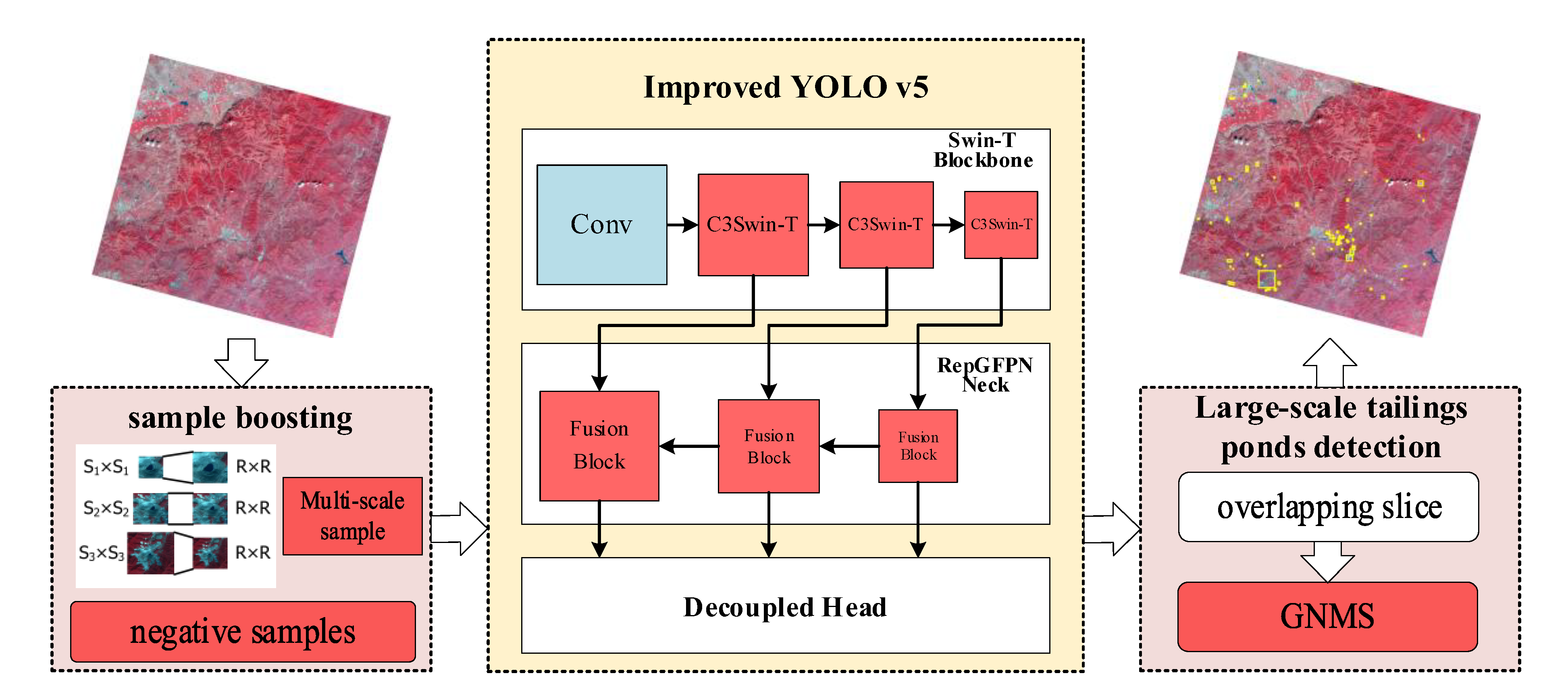
In summary, the research on tailings ponds detection has been carried out in depth, but there are still some challenges. Traditional methods are designed based on the spectral or texture features of tailings ponds, and it is difficult to obtain good detection results in a large area due to excessive changes in tone, shape and dimension between tailings ponds [20]. The application of deep learning methods in tailings pond detection has greatly improved the effect of tailings detection. However, due to the lack of a public tailings sample dataset, and the sparse distribution of tailings ponds with various scales, it is still difficult to accurately detect tailings ponds in a large area. More importantly, with the increase of high-resolution remote sensing data and their cost reduction, target detection based on the entire high-resolution remote sensing image will become one of the mainstream directions of research and engineering. To address the aforementioned limitations on extracting tailings ponds, we propose a framework for detecting tailings ponds from the entire remote sensing image based on the improved YOLOv5 model, which can achieve better detection results than the general YOLOv5.

Our contribution can be summarized as follows:

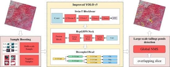
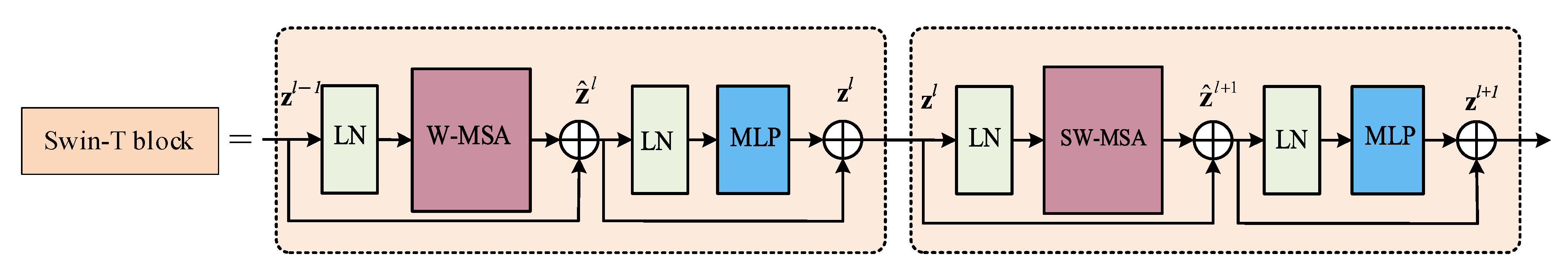
(1) Combine Swin Transformer and C3 to form the new C3Swin-T module, and use the C3Swin-T module to construct Swin-T Blockbone as the backbone of YOLOv5s, which is used to capture sparse tailing pond targets in complex backgrounds.

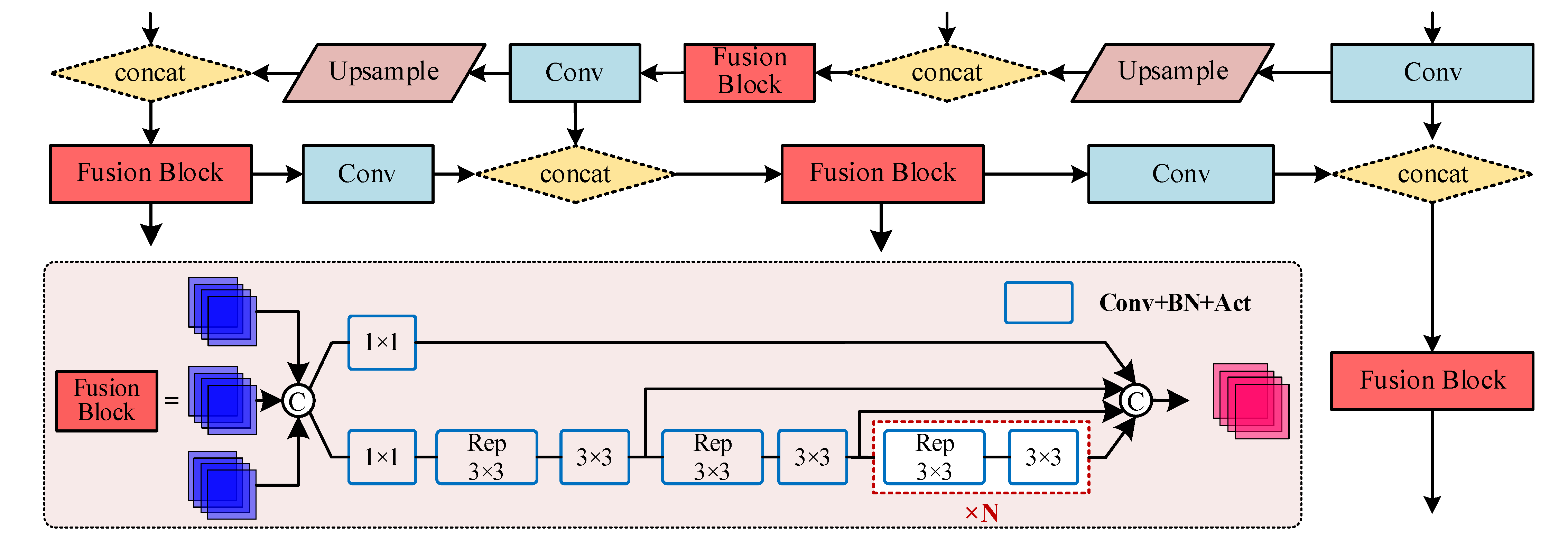
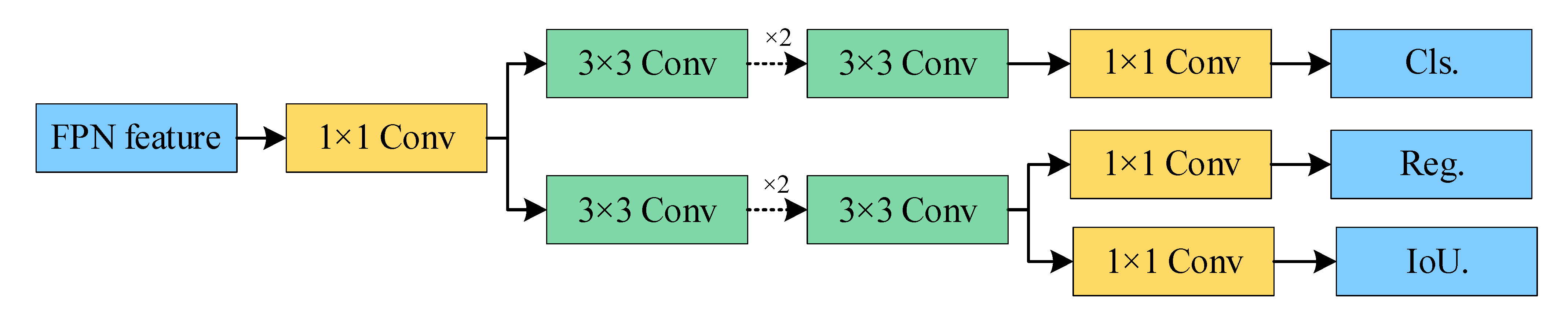
(2) Introduce the Fusion Block in DAMO-YOLO to replace the C3 module of the neck to form RepGFPN Neck, which is used to improve the feature fusion effect of the neck. Replace the original head with Decoupled Head to improve the detection accuracy and model convergence speed.

(3) The SBS and GNMS strategies are proposed to improve the sample quality and suppress repeated detection frames in the whole scene image, respectively, so as to adapt to tailings ponds detection in standard remote sensing images.

2. Study Area and Data

2.1. Study Area

In this study, Laiyuan County and its surrounding areas are selected as the study area, located northwest of Baoding, Hebei Province, as shown in Figure 1. Hebei Province, which is rich in mineral resources, has the largest number of tailings ponds in China, with various types of tailings, concentrated distributions and high potential risks [21]. At the same time, there are similar ground objects to tailings ponds in this area, such as reservoirs, bare rocks, etc., which significantly affect the precise extraction of tailings ponds. Therefore, the selection of this region is precious for verifying the algorithm’s performance and the actual regulatory needs.

2.2. Data and Preprocessing

The GF-6 satellite was launched on 2 June 2018. The GF-6 satellite is equipped with a 2 m panchromatic/8 m multi-spectral high-resolution camera and a 16 m multi-spectral medium-resolution wide-format camera. In this study, we use data from the 2 m panchromatic/8 m multispectral camera to study tailings ponds detection. The specific index parameters are shown in

Table 1. Parameters of the 2 m panchromatic/8 m multispectral cameras.

Spectral Band	Wavelength (μm)	Spatial Resolution (m)	Swath Width (km)
Pan	0.45–0.90	2	90
Blue	0.45–0.52	8	90
Green	0.52–0.60
Red	0.63–0.69
NIR	0.76–0.90

[22].

The acquired data are derived from the L1A processing level. We use ENVI software (version 5.3) to perform the necessary preprocessing such as radiometric calibration and orthorectification, we did not perform image fusion, and the image spatial resolution is 8 m. Wang et al. [23] showed that the Gaofen-1 (GF-1) standard false-color synthesis was the best band combination for effectively identifying tailings ponds. Since the high spatial resolution camera parameters of GF-6 are similar to those of GF-1, we also used the standard false-color synthesis of GF-6 for the extraction study of tailings ponds in this study. GF-6 image data are 12 bits, and the data are converted to 8 bits.

2.3. Types and Characteristics of Tailings Ponds

Due to the influence of many factors such as the topography, landforms, the minerals mined, the mining technology used, and the scale of the operations, tailings ponds can show different layouts, usually divided into four types: cross-valley, hillside, stockpile, or cross-river [15]. Cross-river tailings ponds are rarely in Hebei Province, and we do not consider this category in this study. GF-6 false-color images showing the features of the other three types of tailings ponds are shown in Figure 2. The three types of tailings ponds are different in shape, and the color is mainly gray-blue in the GF-6 standard false-color image.

3. Materials and Methods

The flowchart of the proposed framework in this study is illustrated in Figure 3. It can be summarized by the following steps: (1) Sample boosting strategy. Considering the size change of the tailings ponds and the interference of similar ground objects, the SBS strategy is introduced, including multi-scale sampling and negative sample addition. (2) Improvement of YOLOv5s network architecture. Integrate Swin Transformer to build Swin-T Blackbone, introduce Fusion Block to form RepGFPN Neck, and replace the head with Decoupled Head. (3) Large-scale tailings ponds detection. The overlapping slicing technique is used to block the entire GF-6 image, and the repeated detection frames are merged with the GNMS strategy, then the merged detection frames are output in vector format. (4) Evaluation methods. Some evaluation indicators for model performance are used to evaluate the proposed tailings ponds detection framework.

3.1. Sample Boosting Strategy

In this study, we label a total of 1045 tailings ponds based on the characteristics of three types of tailings on the GF-6 image, which are divided into a training set, validation set and test set according to the ratio of 8:1:1. The sample set contains some samples covering the local area of the tailings ponds to detect incomplete tailings ponds in different image slices well. To realize the purpose of tailings pond detection, the GF-6 image is first sliced. Considering the limitation of computing hardware such as the graphics processing unit memory, the size of the slice samples is set to 500 × 500 pixels. The fixed size of the receptive field limits the observation scale and is harmful to capture scale-dependent information [24], and the relative spatial relationship of the objects helps to improve the recognition accuracy of the target [25,26]. Accordingly, for improving the detection accuracy of tailings ponds, a multi-scale sample sampling strategy needs to be introduced. To facilitate sample preparation, this study adopts the following formula to obtain different scales:

$$S=R\alpha$$

(1)

where R is the sample size we specified, which is 500 × 500 pixels. α is the scaling factor. Once α is determined, samples of size S can be obtained, and then stretch to the size of R. Samples of different scales are obtained by adjusting α.

During the model identification of tailings ponds, it is found that there are many misidentifications because some natural or artificial objects were easily confused with tailings ponds. To reduce the false detection of these objects as tailings ponds, we collect 280 of them and mark them as negative samples. Figure 4 shows some examples of negative samples of tailings ponds. Negative samples collected can be mainly divided into four categories in this study area: water reservoir, bare rock, bare land, and cloud.

3.2. Improvement of YOLOv5s Network Architecture

3.2.1. The Algorithm Principle of YOLOv5

The YOLO family has many models, but they perform differently on different datasets. YOLOv5 is easy to deploy and train, has good reliability and stability [27]. At the same time, Web of Science shows that in the past year, YOLOv5-based publications have an absolute advantage and are widely used. Therefore, YOLOv5 is still highly competitive and is chosen in this study for further improvement. YOLOv5 is a prevalent deep learning framework that includes five network models of different sizes: s, m, l, x, and n, which represent different depths and widths of the network. YOLOv5 treats the detection task as a regression problem, using a single neural network to directly predict bounding boxes and classes. Figure 5 shows the network structure of YOLOv5 (v6.0), which is the latest version of YOLOv5. The whole network consists of three basic parts: Backbone, Neck, and Head. Before being fed into the backbone network, the input images are processed with mosaic data augmentation, adaptive image scaling, and adaptive anchors. In this study, the anchor boxes are automatically adjusted to (12,481, 87,128, 147,141), (239,128, 159,221, 289,274) and (343,524, 558,371, 583,587).

The backbone layer is composed of Conv (Conv2d+BatchNorm+SiLU), C3, and Spatial Pyramid Pooling Fast (SPPF) modules. Among them, C3 is the most important module of the backbone layer, and its idea comes from CSPNet [28]. C3 includes two branches: branch one is connected by n Bottleneck modules in series, branch two is a convolutional layer, and then the two branches are spliced together to increase the network depth and greatly enhance the feature extraction ability. At the same time, the C3 application also suppresses the problem of duplication of gradient information in the backbone. The Conv module is the basic convolution module of YOLOv5, which sequentially performs two-dimensional convolution, regularization and activation operations on the input, which is used to assist the C3 module in feature extraction. SPPF connects a variety of fixed block pooling operations to achieve feature fusion of different scales of receptive fields and enhance the feature expression ability of the backbone.

The neck layer consists of a Feature Pyramid Network (FPN) and Path Aggregation Network (PAN) to form a feature pyramid structure. The FPN structure directly transfers strong semantic features from high-level feature maps to low-level feature maps. The PAN structure directly transfers the stronger localization features from the feature maps of lower layers to the feature maps of higher layers. These two structures together enhance the feature fusion ability of the neck network.

The head layer outputs a vector containing the class probability of the target object, the object score, and the bounding box position of that object. The YOLOv5 detection network consists of three detection layers, each of which has feature maps of different sizes for detecting target objects of different sizes.

3.2.2. Swin-T Backbone

In the entire GF-6 image, a large number of small-sized tailings ponds are in general sparsely and non-uniformly distributed, and it is difficult to distinguish them from the surrounding background, which makes tailings ponds extraction challenging. The YOLOv5s model with the C3 module cannot overcome this deficiency well because it lacks the ability to obtain global and contextual information [29], but the transformer can better integrate the semantic information of the contextual and global features, and has a good recognition effect for sparse small targets with complex backgrounds [30,31]. Due to the high-cost calculation of the transformer, Swin Transformer [32] is selected to improve the backbone network of YOLOv5s. The Swin Transformer block is the core of Swin Transformer, mainly composed of two multi-head self-attention (MSA) modules, window-based MSA (W-MSA) and shifted-window MSA (SW-MSA), followed by a 2-layer multilayer perceptron (MLP) with GELU nonlinearity in between. A LayerNorm (LN) layer is applied before each MSA module and each MLP, and a residual connection is applied after each module, as shown in Figure 6. W-MSA uses regular windows to evenly partition the image in a non-overlapping manner, and computes self-attention within each local window. Therefore, W-MSA has linear computational complexity with respect to input image size, rather than a quadratic complexity of the transformer. Although W-MSA reduces the computational effort, it lacks connections across windows. SW-MSA realizes the information interaction between adjacent windows through a shifted window partitioning approach, and finally realizes the perception of global information. To embed the Swin Transformer block into the backbone, inspired by the work of C3NRT [29] and C3-Trans [30], we propose a new C3Swin-T module, which replaces the original Bottleneck block in C3 by the Swin Transformer block. All C3 modules of the original backbone are replaced by C3SwinT to build a new Swin Transformer backbone (Swin-T backbone), while other layers keep the same, and the structure is illustrated in Figure 7.

3.2.3. RepGFPN Neck

The role of the neck is to better integrate the features extracted by the backbone at different stages to improve the ability of the model to detect features at different scales. YOLOv5s adopts the neck of the FPN+PAN structure. To achieve a better fusion effect, some heavier necks were designed, which increase the computation and memory footprints [33]. In our work, we no longer seek to design a new neck module to avoid more connections and fusions among feature pyramids. We adopt a strategy of replacing some modules of the original neck structure. DAMO-YOLO proposed a novel Efficient-RepGFPN, which improves the model effect by optimizing the topology and fusion of the original GFPN [34]. Additionally, DAMO-YOLO uses the designed fusion block module to improve the low efficiency of node stacking operations and realize the optimization of fusion features. Inspired by this, we replace the C3 module with the fusion block module to improve the feature fusion effect of the model. The fusion block is illustrated in Figure 8. The input of the fusion block is two or three layers. After concat, the number of channels is adjusted on two parallel branches through 1 × 1 Conv. The branch below introduces the idea of the feature aggregation module of efficient layer aggregation networks (ELAN), which consists of multiple Rep 3 × 3 Convs and 3 × 3 Convs. Finally, the outputs of different layers are concat and output. Based on the introduction of various strategies such as CSPNet, reparameterization mechanism and multi-layer aggregation, the fusion block greatly improves the effect of feature fusion. Based on the excellent performance of the fusion block, we replaced the four C3 modules in the neck of YOLOv5s with the fusion block to build a new neck called RepGFPN Neck.

3.2.4. Decoupled Head

The head performs the detection of objects in different resolutions to obtain classification and regression prediction results. YOLOv5s uses a coupled head, which implements classification and regression tasks together. In object detection, the conflict between classification and regression tasks is a well-known problem, affecting the network detection accuracy [35,36]. Thus the Decoupled Head module has been applied in YOLOX, which improves the convergence speed of the network while improving the AP [37]. Due to the excellent performance of the Decoupled Head, it has been used in various subsequent YOLO series models [38,39], even the recently released YOLOv8. To obtain better detection results, we introduced the Decoupled Head into YOLOv5s to replace the original coupled head. The Decoupled Head is illustrated in Figure 9. For each level of the FPN feature, first the number of feature channels is first adjusted by a 1 × 1 Conv layer. Then, two parallel 3 × 3 Conv layers are used to separate the classification and regression tasks so that the classification and regression tasks are performed separately. After that, IoU branch is added to the regression branch. The classification, localization, and confidence detection tasks are implemented by 1 × 1 Conv layer in classification and regression. Cls. represents the category corresponding to the object contained in each feature point. Reg. can obtain the prediction frame coordinates; while IoU. is used to judge whether a feature point contains an object. Finally, these three prediction results are stacked and integrated.

3.3. Large-Scale Tailings Ponds Detection

3.3.1. Overlapping Slices of Large-Scale Imagery

The swath width of the GF-6 high spatial resolution camera image is 90 km, so it is not possible to directly detect tailings ponds on the entire image. Object detection on large-scale images usually uses image slicing [40] or sliding window strategies [41]. Image slicing is likely to cause objects that fall on the segmentation line to be truncated, making objects unable to be detected normally. Additionally, sliding window lacks object detection, and it has high temporal complexity and window redundancy [42]. Therefore, an overlapping slice strategy for large-scale imagery is proposed, as shown in Figure 10. In Figure 10, ol is the overlap ratio, s is the size of the slice, and s−ol × s is the sliding step size.

The process of this strategy is to take the upper left corner as the origin, move from left to right, and from top to bottom according to a certain step size and overlap ratio, and slice until the entire GF-6 image is sliced. In order to easily find the positions of tailings ponds in different sub-slices on the whole image, we calculated the coordinates of the upper left corner of different sub-slices and named different sub-images with the calculated coordinates. The formula for calculating the upper left corner coordinates (x_tl, y_tl) is defined as follows:

$$x_{tl}=\left\{\begin{array}{c}w-s,\hspace{1em}s\times j-ol\times s(j-1)>w\\ (s-ol\times s)(j-1),\hspace{1em}\mathit{otherwise}\end{array}\right.$$

(2)

$$y_{tl}=\left\{\begin{array}{c}h-s,\hspace{1em}s\times i-ol\times s(i-1)>h\\ (s-ol\times s)(i-1),\hspace{1em}\mathit{otherwise}\end{array}\right.$$

(3)

where w is the width of the entire image, h is the height of the entire image, ol is the overlap ratio, and i and j are the ith row and jth column of the traversed image, respectively.

3.3.2. Global Non-Maximum Suppression

Non-maximum suppression (NMS) is a common and important algorithm for dealing with border (rectangular box) redundancy, which is used to merge windows that might belong to the same object [43]. Large-scale remote sensing images are divided into many overlapping slices, and some tailings ponds may completely fall into multiple adjacent slices. In other words, the same tailings pond will be detected multiple times, and multiple detection frames will be generated. Inspired by NMS, we design a strategy for global non-maximum suppression (GNMS) to solve this problem. The GNMS steps are as follows: (1) Obtain the global coordinates of the detection frames of the tailings ponds. Based on the coordinates of the tailings ponds in different sub-slices and the coordinates of the upper left corner of the sub-cut, the global coordinates of the tailings ponds in the entire image are obtained. (2) Merge the duplicate detection frames. Compare the coordinates of the detection frames of the same tailings pond, if a large detection frame covers other detection frames, keep the large detection frame and suppress other detection frames. (3) Non-maximum suppression. If the detection frames of the same tailings pond overlap each other and there is no mutual coverage, the non-maximum suppression method is employed for processing; that is, by comparing the scores of different detection frames and the intersection and ratio operation, remove duplicate frames.

3.4. Evaluation Methods

To evaluate the performance of the proposed framework, we evaluate the model both qualitatively and quantitatively. For qualitative evaluation, the model performance is evaluated by comparing the differences between the images detected by different models; that is, comparing the positioning accuracy of the target frame and whether there are missed or false detections. In quantitative evaluation, the leading selected indicators are: precision, recall, and F1 score. The formula is as follows:

$$precision=\frac{TP}{TP+FP}$$

(4)

$$recall=\frac{TP}{TP+FN}$$

(5)

$$F1=\frac{2\times precision\times recall}{precision+recall}$$

(6)

where TP refers to the number of correct identifications by the detection model, FP refers to the number of incorrect or unrecognized identifications, FN refers to the number of wrongly detected tailings ponds targets as other ground objects.

3.5. Experimental Environment

The configuration parameters of the software and hardware platform implemented by the algorithm in this paper are shown in

Table 2. Configuration parameters.

Device	Configuration
Operating system	Windows 10 (64-bit)
Processor	Intel(R) Core(TM) i7-8750H at 3.80 GHz
RAM	16 G
GPU accelerator	Cuda 10.2, cuDNN 7.6.4
GPU	NVIDIA RTX2070, 8 G
Framework	PyTorch 1.8.1
Scripting language	Python 3.7

.

Some critical hyperparameters are investigated, including training steps, warmup epoch, warmup momentum, batch size, optimization algorithm, initial learning rate, momentum, and weight decay.

Table 3. The hyperparameters of the model.

Hyperparameters	Value
training steps	300 epochs
warmup epoch	3
warmup momentum	0.8
batch size during training	16
batch size during testing	32
optimization algorithm	SGD
initial learning rate	0.01
momentum	0.937
weight decay	0.0005

shows the specific hyperparameter settings.

4. Results and Discussion

To evaluate the performance of the proposed tailings pond detection framework, we design two sets of comparative experiments based on the GF-6 satellite tailings pond image sample dataset. In the first set of experiments, we mainly highlight the effect of introducing the GNMS strategy. In the second set of experiments, we mainly tested the performance of introducing the SBS (named YOLOv5s+SBS), and the performance of improved YOLOv5s with SBS (named Improved YOLOv5s+SBS), and compared the two models with original YOLOv5s to highlight the contribution of introducing the SBS and improved model.

4.1. Experimental Results of GNMS

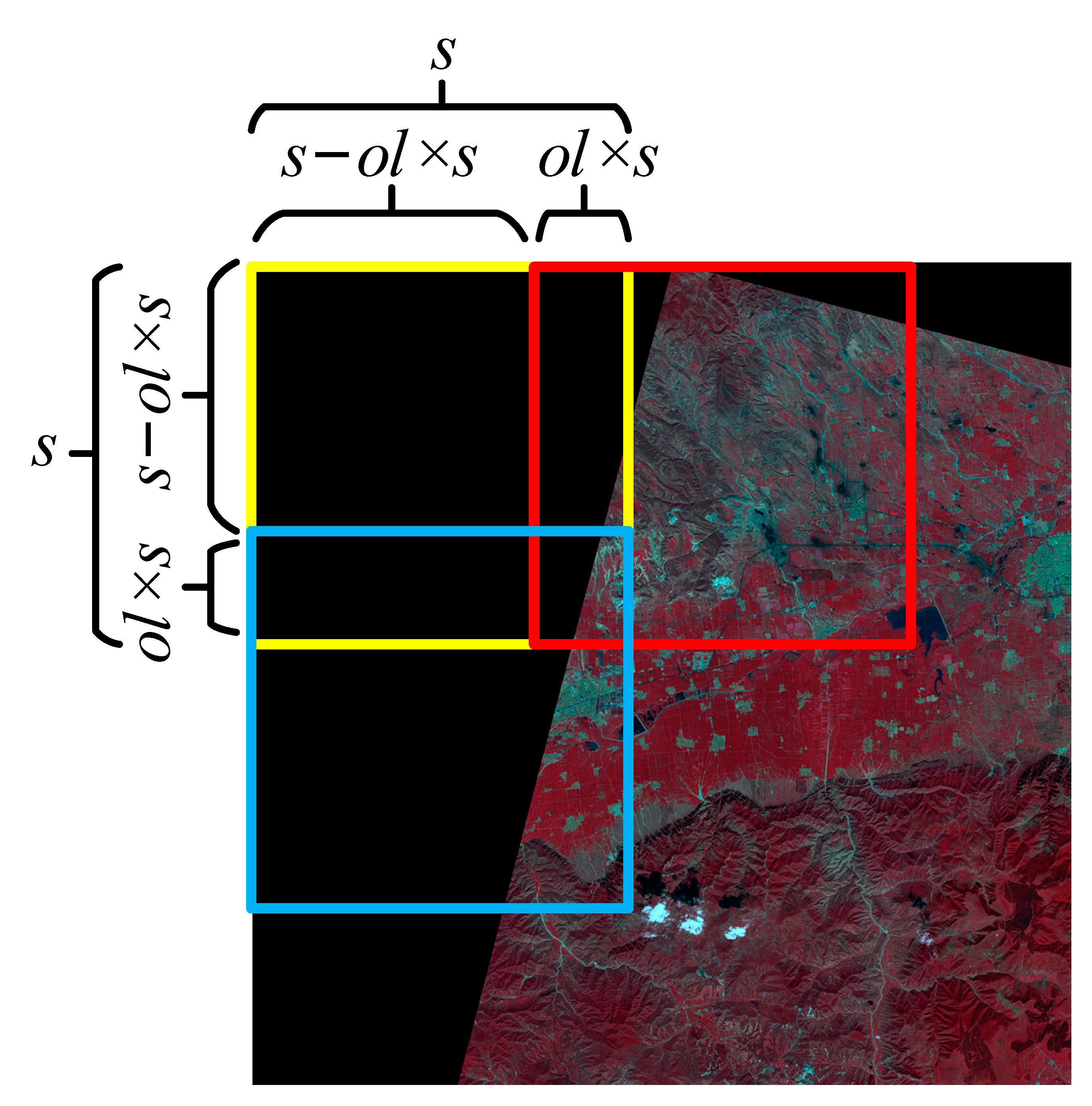
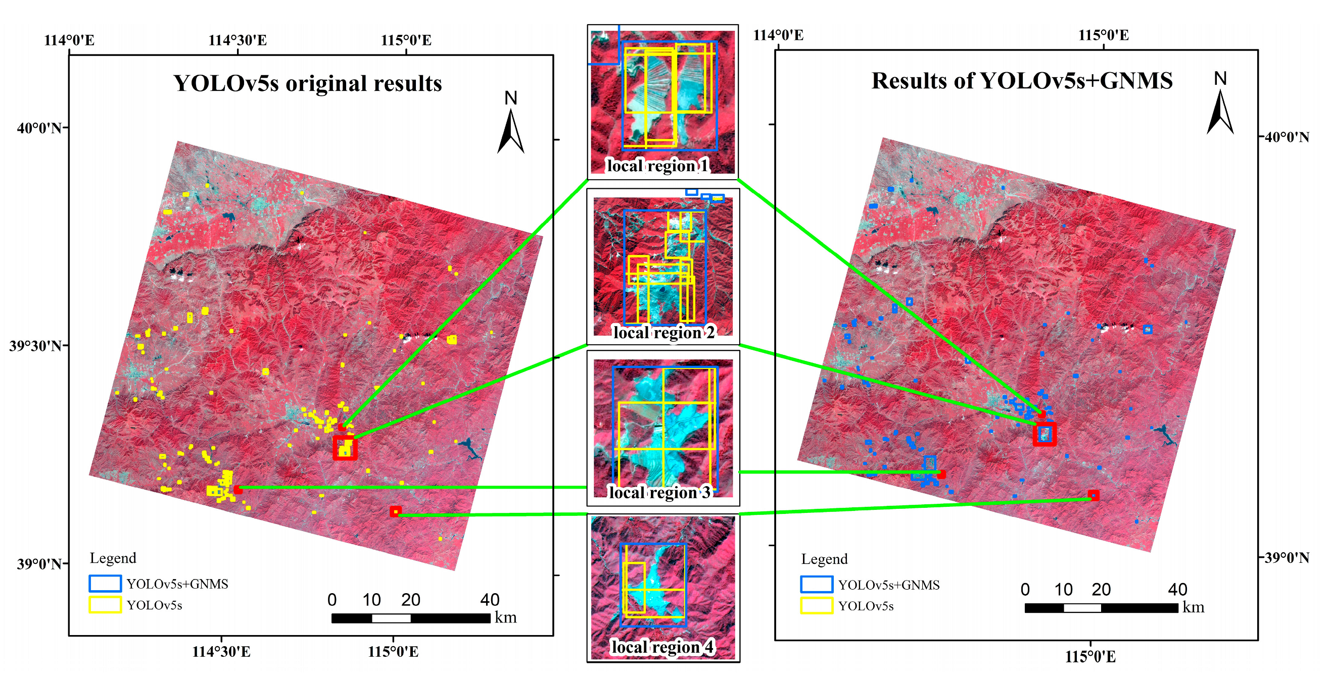
In order to analyze the results of different comparative experiments more objectively, it is necessary to perform GNMS first. In this study, ol is set to 0.2, and the entire remote sensing image is sliced into 3897 image slices. Taking YOLOv5s+SBS as an example, the results of employing the GNMS strategy on the entire GF-6 image are shown in Figure 11. As can be seen from Figure 11, due to the image slice, the tailing ponds are divided into different image slices, and the training samples that focus on the local area of the tailing ponds are added. Many repeated and partial detection frames are generated. GNMS can effectively eliminate duplicate and partial detection frames. Some of these detection frames even exceed the sample size fed to the YOLOv5s model, which can more accurately count the number of real tailings ponds. Compared with the label frames, the error of the detection frames generated by GNMS on the entire GF-6 image is 9.8%.

In order to further observe the performance of GNMS in detail, four local regions are selected for display. The blue detection frames are the experimental results using the GNMS strategy, and the yellow detection frames are original results. In local region 1, the same tailings pond is repeatedly detected many times due to part of the training samples. Most of the detection frames are suppressed using GNMS, but since the two tailings ponds are too close, they are both represented by the same detection frame. The tailings ponds in region 2 and region 3 are large and may be repeatedly detected in different sub-slices, so the generated detection frames are marked on the image. After being processed by GNMS, the detection frame on the same tailings pond will no longer have partial coverage, but full coverage of the tailings pond. In local region 4, we can see that the same tailings pond is repeatedly detected three times, and after processing by GNMS, only one detection frame remains.

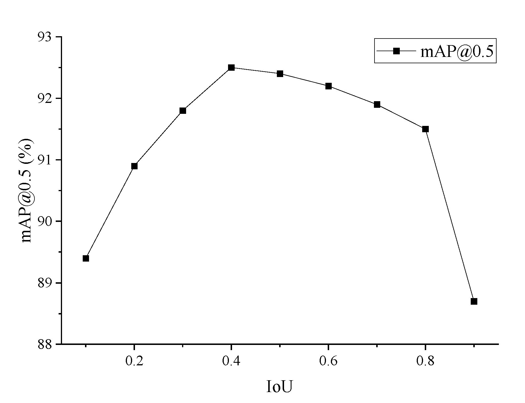
To investigate the effect of the IoU threshold of GNMS on the accuracy of tailings ponds detection, different IoU thresholds are selected to obtain the best mAP@0.5 on the test set. The IoU threshold ranges from (0, 1) with a step size of 0.1, and the results are shown in Figure 12. Figure 12 shows that the mAP@0.5 is maximum when the IoU threshold is 0.4.

4.2. Comparative Results of Different Experiments

4.2.1. Qualitative Results

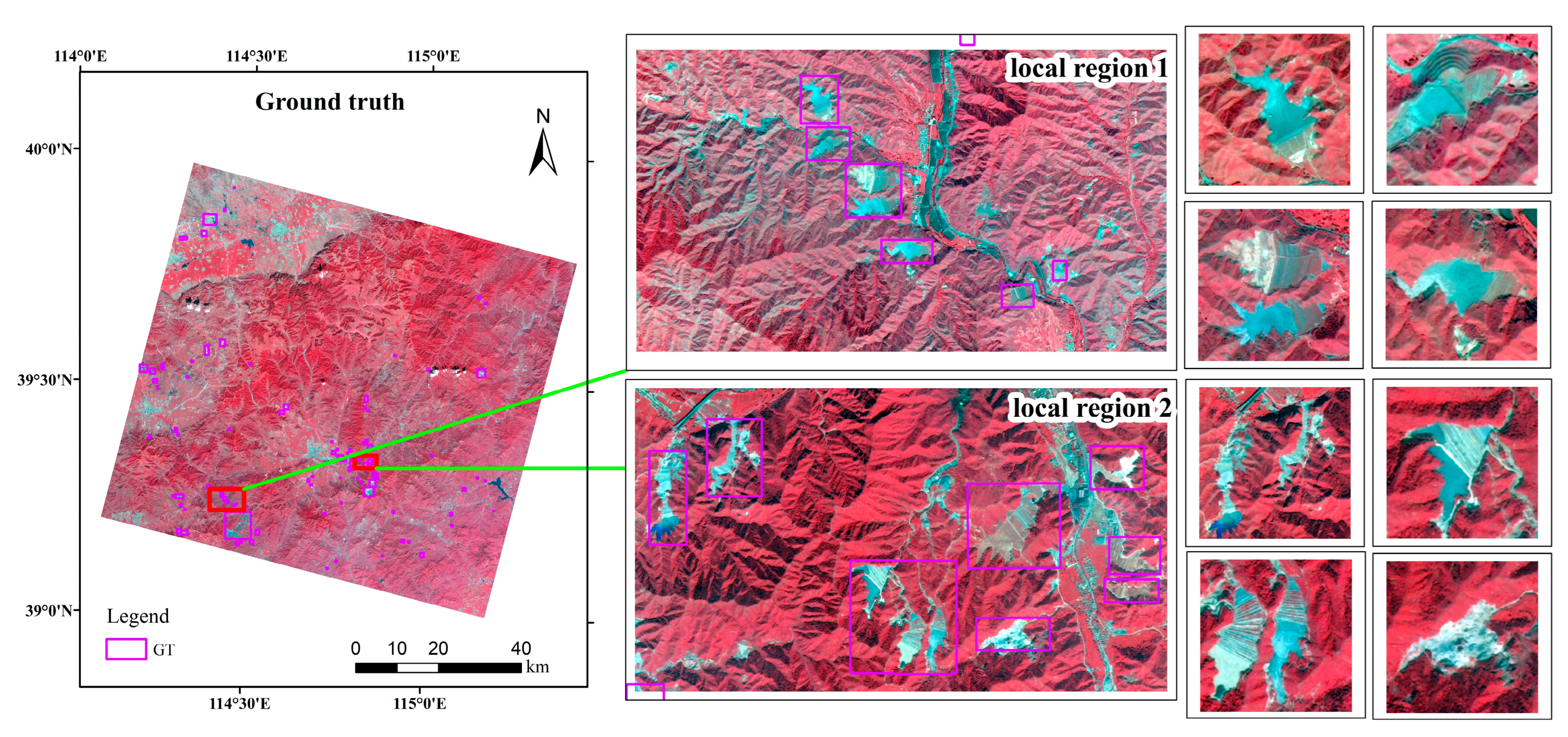
To obtain a more accurate ground truth map, we first marked the location of the tailings ponds on a high-resolution Google Earth map. Based on the precise location information, we marked the label frames of the tailings ponds on the entire GF-6 image. From Figure 13, these label frames are purple. In order to show the truth map more clearly, we selected two typical local regions, and selected four tailings ponds from each region for display. According to a statistical analysis of the size of the marked tailings ponds, their length and width are typically between 70 m and 3000 m.

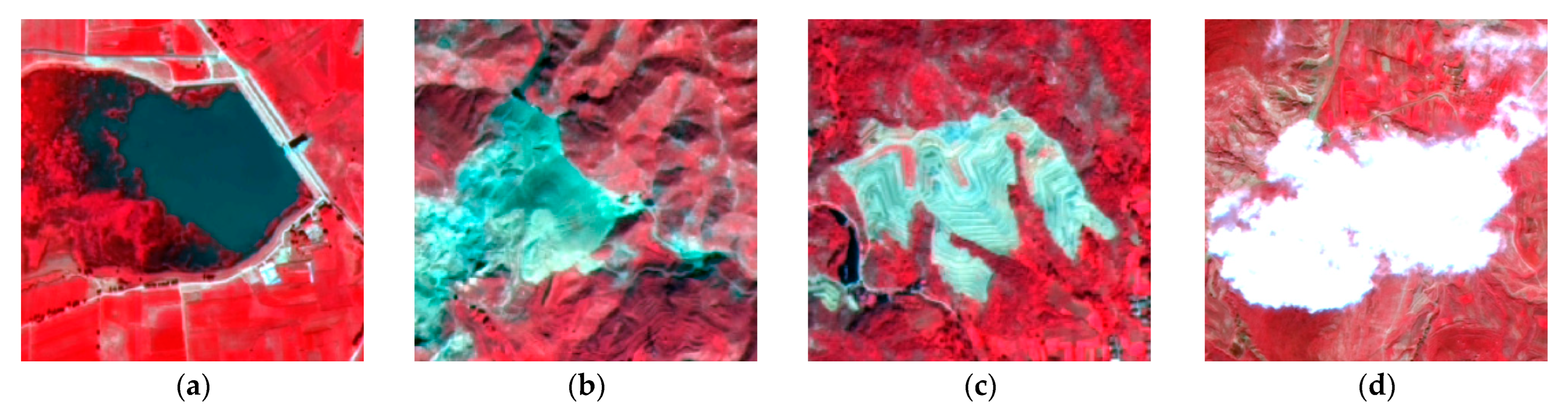
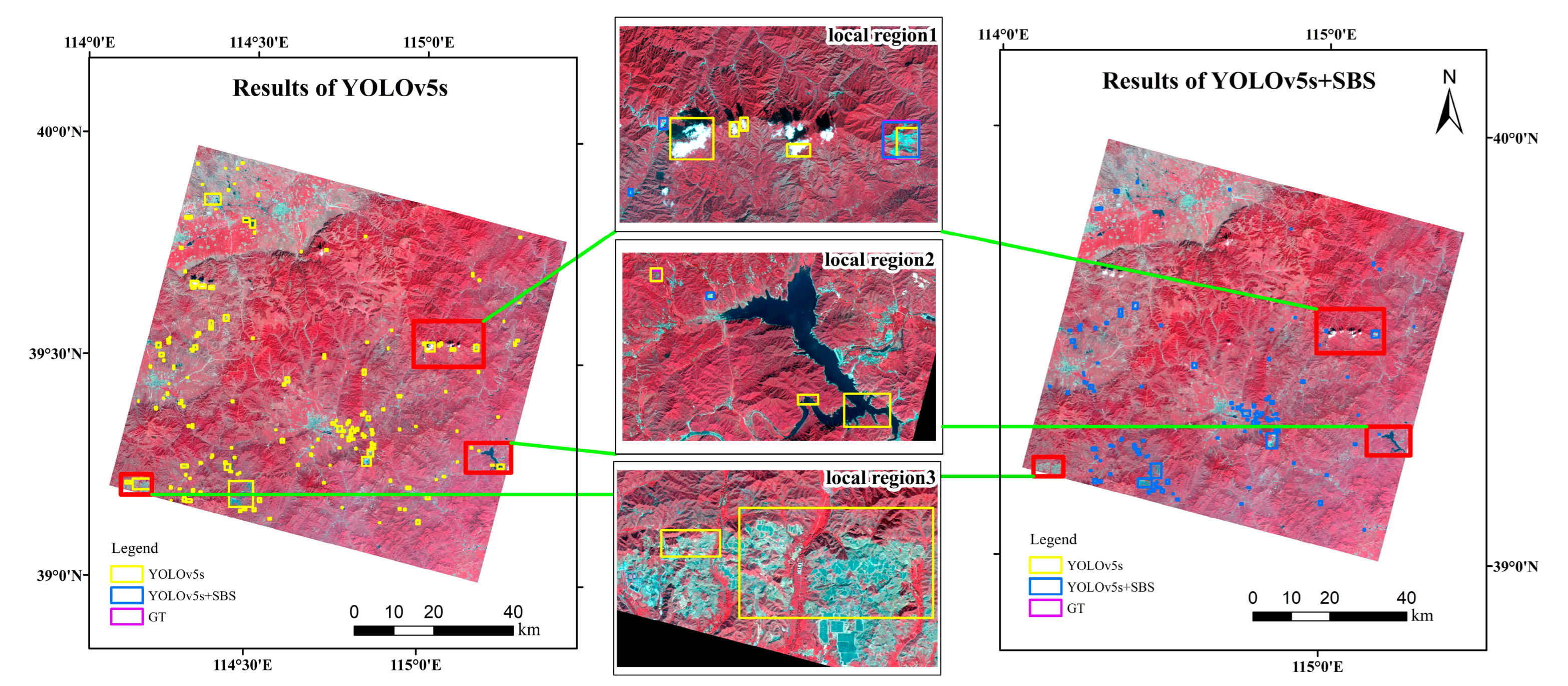
Figure 14 shows the qualitative tailings ponds detection results of YOLOv5s and YOLOv5s+SBS on the entire GF-6 image. Compared with ground truth, the results of the YOLOv5s have more obvious misidentifications. From the results of YOLOv5s, we can see that there are mainly three ground objects that are more misidentified as tailings ponds, namely clouds, reservoirs and bare rocks of mountains. We selected three local regions to display typical errors. Local region 1 is used to show that clouds are misidentified as tailings ponds. Local region 2 is used to show that reservoirs are misidentified as tailings ponds. Local region 3 is used to show that bare rocks are misidentified as tailings ponds. In these three local regions, compared with YOLOv5, the detection results of YOLOv5+SBS can well avoid these obvious errors and obtain better detection results.

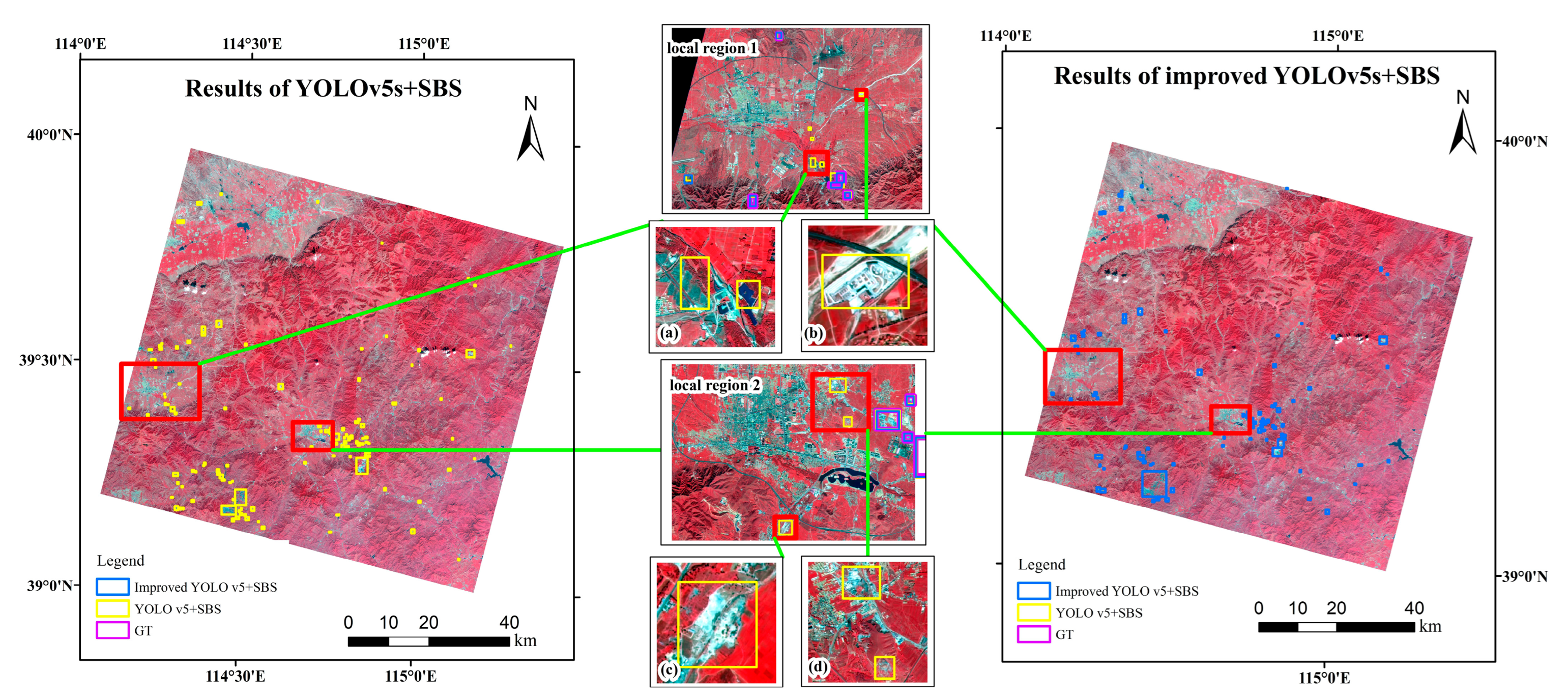
Figure 15 shows the qualitative tailings ponds detection results of YOLOv5s+SBS and improved YOLOv5s+SBS on the entire GF-6 image. Compared with the YOLOv5s model, YOLOv5s+SBS has significantly improved the erroneous extraction of tailings ponds, but there are also several obvious erroneous extractions. Through observation, these misidentified ground objects are mainly concentrated near residential areas, and scattered in other areas, mainly bare land and buildings. We selected two local regions around Lingqiu County and Laiyuan County to show the results. Region 1 is Lingqiu County and region 2 is Laiyuan County. In order to show the detection results more clearly, we selected two sub-areas (a) and (b) in local region 1, and two sub-regions (c) and (d) in local region 2. In sub-region (a), the YOLOv5s+SBS model misidentifies the bare land in the left detection frame and the pond in the right detection frame as tailings ponds. In sub-region (b), the YOLOv5s+SBS model misidentifies a factory in the detection frame as a tailings pond. In both sub-region (c) and (d), the YOLOv5s+SBS model misidentifies the bare land as a tailings pond. Compared with YOLOv5+SBS, the detection results of improved YOLOv5+SBS can obtain better detection results.

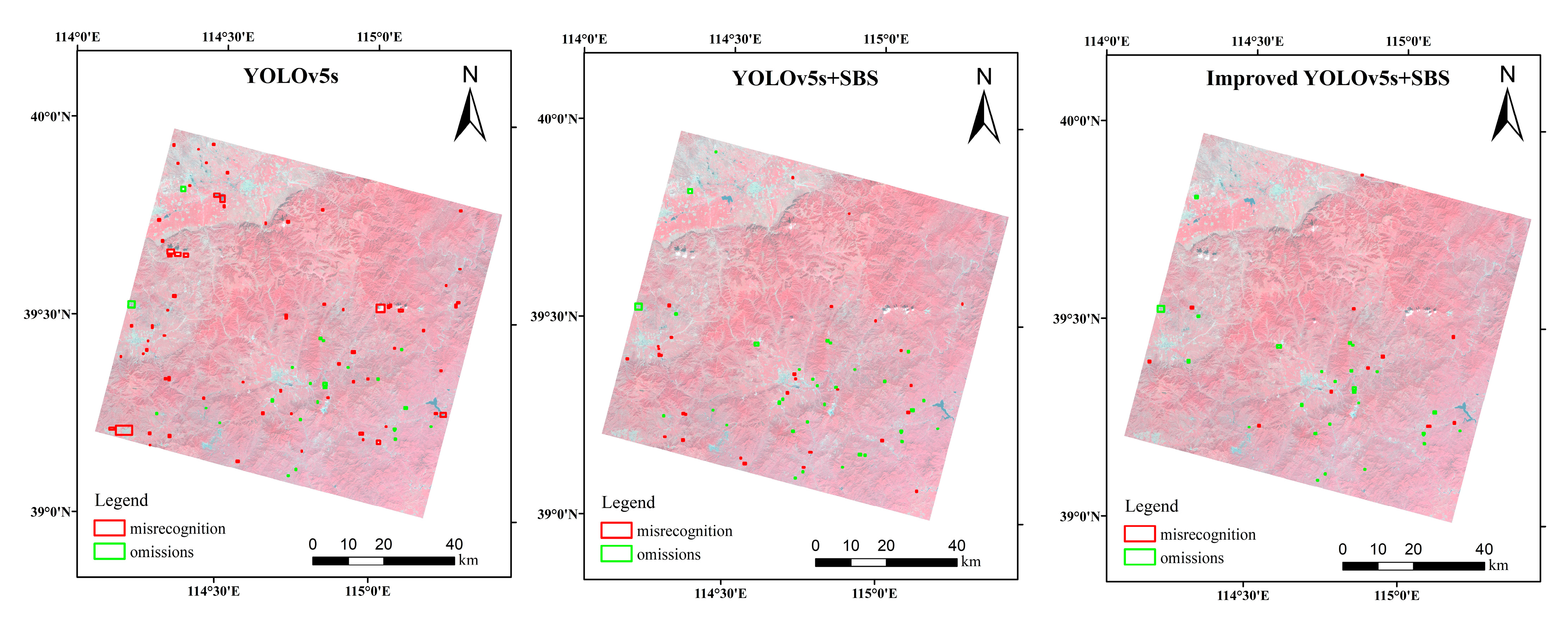
In order to overall compare the performance of the three models, we show the results of misrecognition and omissions of different models, respectively, on the entire GF-6 image. Red detection frames represent misrecognition, and green detection frames represent omissions. From Figure 16, the misrecognition of YOLOv5s is the highest, followed by YOLOv5s+SBS, and our framework has achieved the best performance. YOLOv5s has about the same number of omissions as our framework, while YOLOv5+SBS has relatively more omissions.

4.2.2. Quantitative Results

In this study, a counting method is used for performance evaluation. We use the GF-6 image with label frames as a ground truth map, as shown in Figure 13. If the detection frame predicted by the models intersects with the label frame, we consider the detection frame predicted by the model to be correctly identified and denote it as TP; if there is no intersection between the detection frame and the labeled frame, and it is identified as other ground objects, it is judged as a misrecognition, which is denoted as FP; if the labeled frames are not detected, they are judged as missing and denoted as FN. We obtain quantitative comparison results of different models using the calculation formula for accuracy evaluation, see

Table 4. Performance comparison of different models.

Models	Precision	Recall	F1	Iteration Time
YOLO v5	61.02%	81.20%	69.68%	58.05 s
YOLO v5+SBS	78.34%	75.54%	76.91%	58.07 s
Improved YOLO v5+SBS	86.00%	78.18%	81.90%	166.01 s

.

From Table 4, the accuracy of the proposed framework has been greatly improved by introducing the SBS and improving YOLOv5s. Compared with the original YOLOv5s, the F1 score has increased by 12.22%, and the precision has increased by nearly 25%, but the recall is lower than YOLOv5s. Compared with the YOLOv5s+SBS, the F1 score has increased by about 5%, the precision has increased by 7.66%, and the recall has increased by 2.64%. However, compared to the other two models, the proposed framework increases the detection execution time of tailings ponds on the entire GF-6 image by about three times. It should be pointed out that the final detection result is saved in vector format, not in raster format. It not only improves the detecting efficiency and saves storage space, but also can be easily superimposed on any map with a coordinate system for display.

4.3. Discussion

In this study, YOLOv5s is comprehensively improved, combining the strategies of SBS and GNMS, and innovatively designing a new framework for large-scale tailings ponds extraction from the entire remote sensing image. Our framework achieves the best performance in comparative experiments. Although the execution time is the longest, an entire GF-6 image is about 90 km by 90 km in size, and it takes about 166 s, which is acceptable. In this subsection, it is clarified that all models employ SBS.

4.3.1. Ablation Experiment

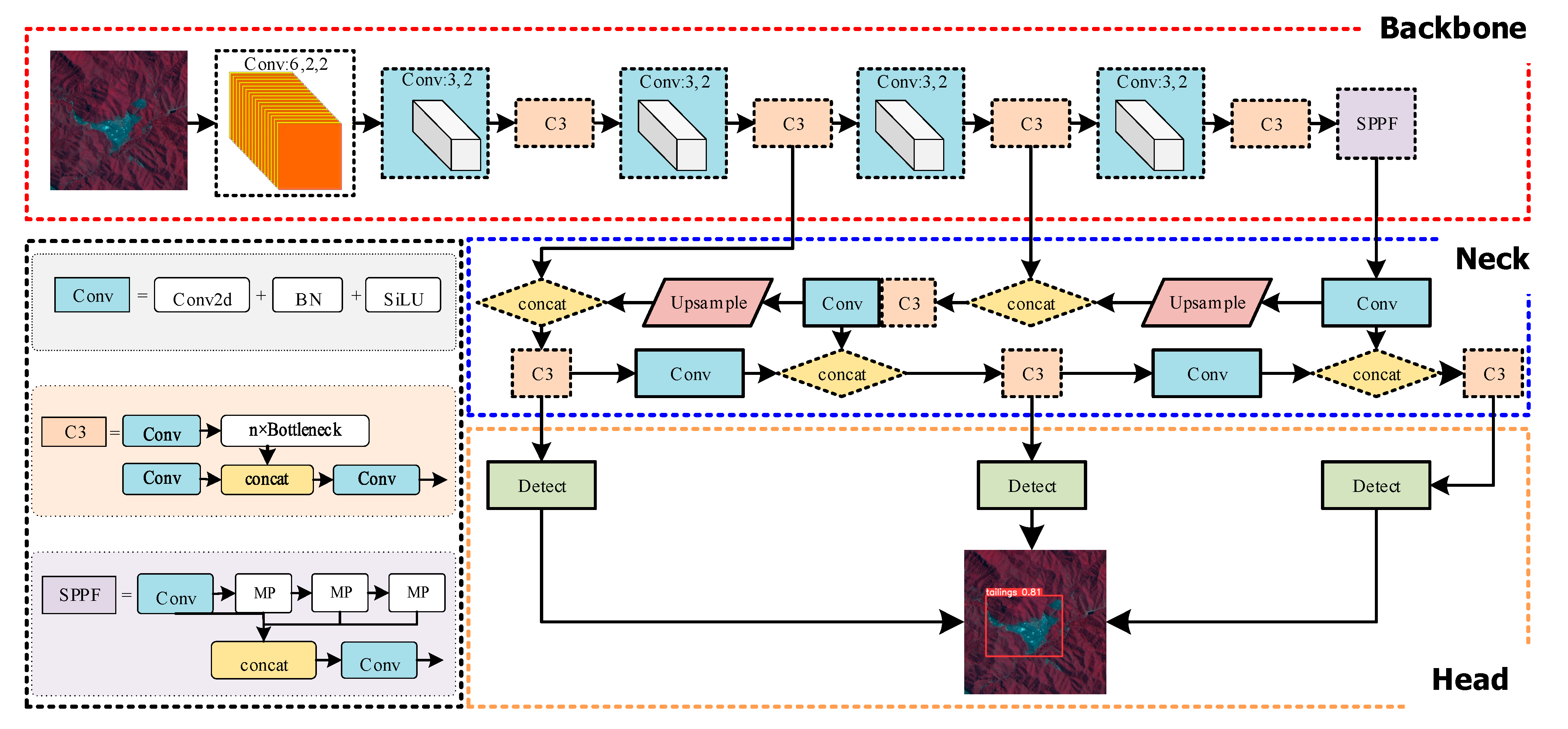
There are many improvement measures in our model, including: replacing C3 with C3SwinT module in backbone, replacing C3 with fusion block module in neck, and replacing the coupled head with Decoupled Head. To verify the effect of these measures on the improved YOLOv5s, an ablation experiment is undertaken in this paper. Additionally, the mAP@0.5 and number of parameters are used as evaluation indexes. For fair comparison, default parameters are used for all models. The final results are listed in

Table 5. Results of ablation experiments.

Model	Parameters (M)	mAP@0.5	Improvement over YOLOv5s
YOLOv5s (baseline)	7.03	86.20%	-
+Swin-T Backbone	7.27	90.20%	4%
+RepGFPN Neck	12.25	89.60%	3.4%
+Decoupled Head	14.33	88.20%	2%
Ours	19.82	92.15%	5.95%

.

Compared with the baseline network, the improved YOLOv5s boosts mAP@0.5 by 5.95%. Although our model has the highest mAP@0.5 of 92.15%, it has the largest number of parameters. YOLOv5 with Swin-T Backbone achieves 90.20% mAP@0.5, an increase of 4% mAP@0.5 compared with the baseline network, and the number of parameters of the model is slightly increased. YOLOv5 with RepGFPN Neck achieved 89.60% mAP@0.5, mAP@0.5 increased by 3.4%, and the number of parameters increased by 5.22 M. In comparison with the baseline network, YOLOv5 with Decoupled Head improved 2% mAP@0.5, and the number of parameters increased by 7.3 M, second only to our model. It can be seen that the improvement of different parts of YOLOv5 has achieved an increase of mAP@0.5. Swin-T Backbone contributed the most, showing that Swin Transform has a good effect on extracting sparse targets in complex background images. The contribution of RepGFPN Neck is second, indicating that this new feature fusion mode that transfers node stacking calculations to convolutional layer stacking calculations is very effective in target recognition on remote sensing images. Decoupled Head also cannot be ignored, and it is an important means to improve the accuracy of target detection.

4.3.2. Comparison with Other Object Detection Methods

To demonstrate the effectiveness of the improved YOLOv5s in detecting tailings ponds on GF-6 images, this study compares the performance of our method with that of several other state-of-the-art (SOTA) object detection methods, such as YOLOv8s, YOLOv5l, YOLT [44] and the Swin Transformer [32], on the GF-6 self-made tailing pond dataset.

Table 6. Experimental results of comparative experiments.

Model	Parameters (M)	mAP@0.5
YOLOv5l	46.11	87.60%
YOLOv8s	11.13	88.00%
YOLTv5s	7.06	88.60%
Swin-T	47.37	88.70%
Ours	19.82	92.15%

shows the performance comparison of different methods.

From Table 6, compared to several other SOTA methods, our improved YOLOv5s obtains the highest mAP@0.5, followed by Swin Transformer and YOLTv5s. For Swin Transformer, the backbone we choose is Swin-T with Lr Schd 3x. YOLTv5 is the fifth version of YOLT, developed based on YOLOv5, and we also chose the size of s. YOLOv8s achieved 88.00% mAP@0.5, which is the latest YOLO released by the community. It adopts the new C2f module and decoupled head, and has a very good performance. Compared with YOLOv5s, YOLOv5l has a larger model depth multiple and layer channel multiple, which can usually achieve better detection results. It should be noted that default hyperparameters were used for all compared models. Although Swin Transformer has achieved sub-optimal performance, it has a large number of parameters. After fusing it with C3, it can maintain a good extraction accuracy and greatly reduce the number of parameters. YOLTv5s can still achieve good detection results while maintaining the same number of parameters as YOLOv5s. YOLOv8s has a small number of parameters and has achieved good detection results. The number of parameters of YOLOv5l is almost the same as that of Swin Transformer, but its improvement of mAP@0.5 is relatively small. In general, our improved YOLOv5 has a great advantage in the task of detecting tailings ponds on GF-6 images.

In order to further analyze the recognition performance of the proposed model for tailings ponds, our model is also compared with the improved YOLOv8s. We replace the C2f modules of the YOLOv8s backbone with C3SwinT modules to form Swin-T Backbone, and replaced the C2f modules of the YOLOv8s neck with fusion block modules to form RepGFPN Neck. From

Table 7. Comparison of improved YOLOv5s and YOLOv8s.

Model	YOLOv5s		YOLOv8s
	Parameters (M)	mAP@0.5	Parameters (M)	mAP@0.5
+Swin-T Backbone	7.27	90.20%	10.29	90.10%
+RepGFPN Neck	12.25	89.60%	15.37	89.30%
Improved Model	19.82	92.15%	14.51	90.06%

, the first row represents YOLOv5s and YOLOv8s with Swin-T Backbone, the second row represents YOLOv5s and YOLOv8s with RepGFPN Neck, and the third row represents improved YOLOv5s and YOLOv8s with Swin-T Backbone, RepGFPN Neck and Decoupled Head. It should be pointed out that YOLOv8s has Decoupled Head, and the improved YOLOv8s only employs Swin-T Backbone and RepGFPN Neck. Compared with different improved YOLOv8s models, different improved YOLOv5s models have higher mAP@0.5, and the parameters of the models also have certain advantages.

4.3.3. Limitations and Future Works

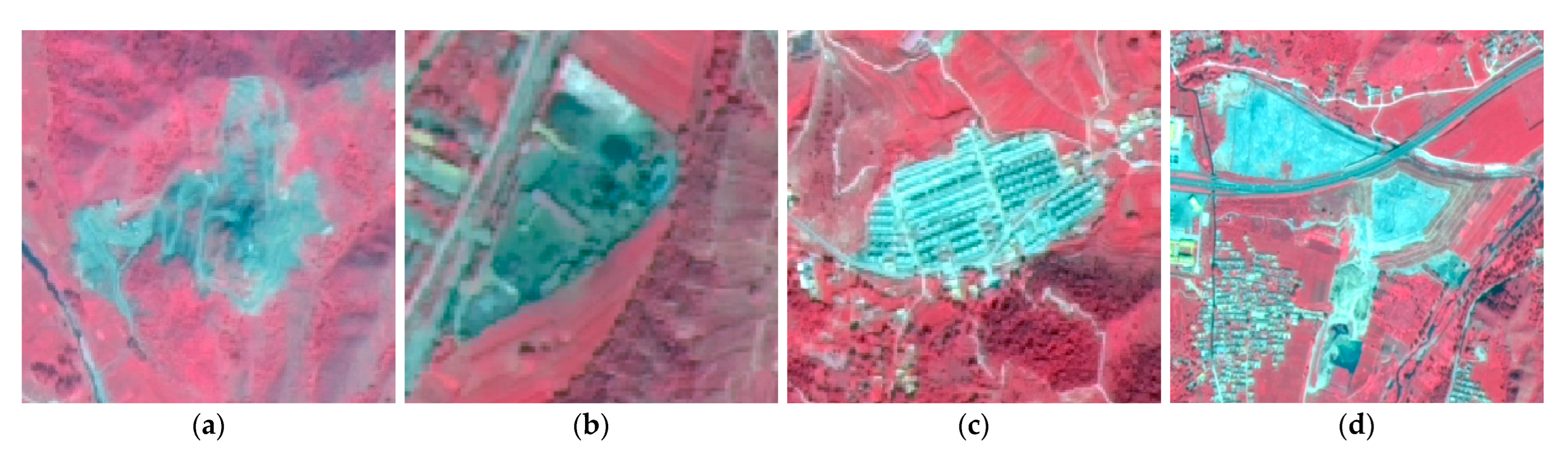
Although our framework obtained the best accuracy for tailings ponds identification, there are still misidentifications, and the detection of tailings ponds in a large area still faces challenges. Figure 17 shows some typical cases misidentified by our framework, such as bare soil, factories, residential areas, and highway service areas, which are morphologically and spectrally similar to tailings ponds. In addition, the phenomenon of missing extraction of the framework cannot be ignored, and the typicality of these undetected tailings ponds is often not prominent enough, which is also worthy of attention and research in the future.

Furthermore, we generated a dataset of tailings ponds based on standard false-color images of the GF-6 high-resolution camera, which is still small-scale and not particularly general compared to other public datasets of ground objects. In the future, it is necessary to establish large-scale tailings pond dataset based on GF-6 standard false-color images and explore specific data enhancement methods. Apart from some misidentifications and omissions, our framework lacks competition in the number of model parameters and detection time. We hope to carry out model pruning and knowledge distillation in the future to improve model efficiency and meet more application scenarios. In addition, tailings ponds have strong spatial heterogeneity, and the characteristics of tailings ponds in different regions are quite different. Therefore, the fusion of multi-source data, such as hyperspectral data, are used to more finely detect tailings ponds in larger areas.

5. Conclusions

This study proposes an improved YOLOv5s framework for tailings ponds extraction from the entire GF-6 high spatial resolution remote sensing image. The proposed SBS technique improves the quality of the tailings ponds image sample dataset by adding multi-scale samples and negative samples. The improved YOLOv5s consists of Swin-T Backbone, RepGFPN Neck and Decoupled Head. The C3Swin-T module formed by Swin Transformer and C3 can well-capture the features of sparse tailing pond targets in complex backgrounds. Fusion Block can achieve better feature fusion effects by introducing strategies such as CSPNet, reparameterization mechanism, and multi-layer aggregation. Decoupled Head replacing a coupled head also achieved better results. In addition, the designed GNMS can effectively suppress the repeated detection frames on the entire remote sensing image and improve the detection effect. The results show that the precision and F1 score of tailings ponds detection using the improved framework are significantly improved, which are 24.98% and 12.22%, respectively, compared with the original YOLOv5s, and 7.66% and 4.99%, respectively, compared with YOLOv5s+SBS, reaching 86.00% and 81.90%, respectively. Our framework can provide an effective method for government departments to conduct a tailings ponds inventory, and provide a useful reference for mine safety and environmental monitoring.

References

1. Che, D.; Liang, A.; Li, X.; Ma, B. Remote Sensing Assessment of Safety Risk of Iron Tailings Pond Based on Runoff Coefficient. Sensors 2018, 18, 4373. [Google Scholar] [CrossRef] [PubMed] [Green Version]
2. Komnitsas, K.; Kontopoulos, A.; Lazar, I.; Cambridge, M. Risk assessment and proposed remedial actions in coastal tailings disposal sites in Romania. Miner. Eng. 1998, 11, 1179–1190. [Google Scholar] [CrossRef]
3. Yu, D.; Tang, L.; Ye, F.; Chen, C. A virtual geographic environment for dynamic simulation and analysis of tailings dam failure. Int. J. Digit. Earth 2021, 14, 1194–1212. [Google Scholar] [CrossRef]
4. Morgan, G.; Gomes, M.V.P.; Perez-Aleman, P. Transnational governance regimes in the global south: Multinationals, states and NGOs as political actors. Rev. Adm. Empresas 2016, 56, 374–379. [Google Scholar] [CrossRef] [Green Version]
5. Burritt, R.L.; Christ, K.L. Water risk in mining: Analysis of the Samarco dam failure. J. Clean. Prod. 2018, 178, 196–205. [Google Scholar] [CrossRef]
6. Xiao, R.; Shen, W.; Fu, Z.; Shi, Y.; Xiong, W.; Cao, F. The application of remote sensing in the environmental risk monitoring of tailings pond: A case study in Zhangjiakou area of China. In Earth Resources and Environmental Remote Sensing/GIS Applications III; SPIE: Edinburgh, UK, 2012. [Google Scholar] [CrossRef]
7. Hu, X.; Oommen, T.; Lu, Z.; Wang, T.; Kim, J.-W. Consolidation settlement of Salt Lake County tailings impoundment revealed by time-series InSAR observations from multiple radar satellites. Remote Sens. Environ. 2017, 202, 199–209. [Google Scholar] [CrossRef]
8. Rotta, L.H.S.; Alcântara, E.; Park, E.; Negri, R.G.; Lin, Y.N.; Bernardo, N.; Mendes, T.S.G.; Filho, C.R.S. The 2019 Brumadinho tailings dam collapse: Possible cause and impacts of the worst human and environmental disaster in Brazil. Int. J. Appl. Earth Obs. Geoinf. 2020, 90, 102119. [Google Scholar] [CrossRef]
9. Cheng, D.; Cui, Y.; Li, Z.; Iqbal, J. Watch Out for the Tailings Pond, a Sharp Edge Hanging over Our Heads: Lessons Learned and Perceptions from the Brumadinho Tailings Dam Failure Disaster. Remote Sens. 2021, 13, 1775. [Google Scholar] [CrossRef]
10. Lévesque, J.; Neville, R.A.; Staenz, K.; Truong, Q.S. Preliminary results on the investigation of hyperspectral remote sensing for the identification of uranium mine tailings. In Proceedings of the ISSSR, Quebec City, QC, Canada, 10–15 June 2001; pp. 10–15. [Google Scholar] [CrossRef]
11. Ma, B.; Chen, Y.; Zhang, S.; Li, X. Remote Sensing Extraction Method of Tailings Ponds in Ultra-Low-Grade Iron Mining Area Based on Spectral Characteristics and Texture Entropy. Entropy 2018, 20, 345. [Google Scholar] [CrossRef] [Green Version]
12. Hao, L.; Zhang, Z.; Yang, X. Mine tailing extraction indexes and model using remote-sensing images in southeast Hubei Province. Environ. Earth Sci. 2019, 78, 1–11. [Google Scholar] [CrossRef] [Green Version]
13. Liu, K.; Liu, R.; Liu, Y. A Tailings Pond Identification Method Based on Spatial Combination of Objects. IEEE J. Sel. Top. Appl. Earth Obs. Remote Sens. 2019, 12, 2707–2717. [Google Scholar] [CrossRef]
14. Wu, X. Image Extraction of Tailings Pond Guided by Artificial Intelligence Support Vector Machine. Wirel. Commun. Mob. Comput. 2022, 2022, 1–11. [Google Scholar] [CrossRef]
15. Li, Q.; Chen, Z.; Zhang, B.; Li, B.; Lu, K.; Lu, L.; Guo, H. Detection of Tailings Dams Using High-Resolution Satellite Imagery and a Single Shot Multibox Detector in the Jing–Jin–Ji Region, China. Remote Sens. 2020, 12, 2626. [Google Scholar] [CrossRef]
16. Balaniuk, R.; Isupova, O.; Reece, S. Mining and Tailings Dam Detection in Satellite Imagery Using Deep Learning. Sensors 2020, 20, 6936. [Google Scholar] [CrossRef] [PubMed]
17. Ferreira, E.; Brito, M.; Balaniuk, R.; Alvim, M.S.; Santos, J.A.D. Brazildam: A benchmark dataset for tailings dam detection. In Proceedings of the 2020 IEEE Latin American GRSS & ISPRS Remote Sensing Conference (LAGIRS), Santiago, Chile, 22–26 March 2020; IEEE: New York, NY, USA, 2020. [Google Scholar]
18. Yan, D.; Li, G.; Li, X.; Zhang, H.; Lei, H.; Lu, K.; Cheng, M.; Zhu, F. An Improved Faster R-CNN Method to Detect Tailings Ponds from High-Resolution Remote Sensing Images. Remote Sens. 2021, 13, 2052. [Google Scholar] [CrossRef]
19. Yan, D.; Zhang, H.; Li, G.; Li, X.; Lei, H.; Lu, K.; Zhang, L.; Zhu, F. Improved Method to Detect the Tailings Ponds from Multispectral Remote Sensing Images Based on Faster R-CNN and Transfer Learning. Remote Sens. 2021, 14, 103. [Google Scholar] [CrossRef]
20. Lyu, J.; Hu, Y.; Ren, S.; Yao, Y.; Ding, D.; Guan, Q.; Tao, L. Extracting the Tailings Ponds From High Spatial Resolution Remote Sensing Images by Integrating a Deep Learning-Based Model. Remote Sens. 2021, 13, 743. [Google Scholar] [CrossRef]
21. Tang, L.; Liu, X.; Wang, X.; Liu, S.; Deng, H. Statistical analysis of tailings ponds in China. J. Geochem. Explor. 2020, 216, 106579. [Google Scholar] [CrossRef]
22. Lasac, M. Gaofen-6 Satellite. 2018. Available online: http://sasclouds.com/chinese/satellite/chinese/gf6 (accessed on 26 January 2023).
23. Wang, J.; Cao, L.; Guo, Y.; Zhao, L.; Wu, B. Feature analysis and information identification of the iron tailings by high−multispectral remote sensing. J. Yunnan Univ. Nat. Sci. Ed. 2019, 41, 974–981. [Google Scholar]
24. Fauvel, M.; Chanussot, J.; Benediktsson, J. A spatial–spectral kernel-based approach for the classification of remote-sensing images. Pattern Recognit. 2012, 45, 381–392. [Google Scholar] [CrossRef]
25. Zhong, Y.; Fei, F.; Zhang, L. Large patch convolutional neural networks for the scene classification of high spatial resolution imagery. J. Appl. Remote Sens. 2016, 10, 25006. [Google Scholar] [CrossRef]
26. Liu, Y.; Zhong, Y.; Fei, F.; Zhu, Q.; Qin, Q. Scene Classification Based on a Deep Random-Scale Stretched Convolutional Neural Network. Remote Sens. 2018, 10, 444. [Google Scholar] [CrossRef] [Green Version]
27. Liu, Z.; Gao, X.; Wan, Y.; Wang, J.; Lyu, H. An Improved YOLOv5 Method for Small Object Detection in UAV Capture Scenes. IEEE Access 2023, 11, 14365–14374. [Google Scholar] [CrossRef]
28. Wang, C.-Y.; Liao, H.-Y.M.; Wu, Y.-H.; Chen, P.-Y.; Hsieh, J.-W.; Yeh, I.-H. CSPNet: A new backbone that can enhance learning capability of CNN. In Proceedings of the IEEE/CVF Conference on Computer Vision and Pattern Recognition Workshops, Seattle, WA, USA, 14–19 June 2020. [Google Scholar]
29. Liu, Y.; He, G.; Wang, Z.; Li, W.; Huang, H. NRT-YOLO: Improved YOLOv5 Based on Nested Residual Transformer for Tiny Remote Sensing Object Detection. Sensors 2022, 22, 4953. [Google Scholar] [CrossRef] [PubMed]
30. Zhu, X.; Lyu, S.; Wang, X.; Zhao, Q. TPH-YOLOv5: Improved YOLOv5 Based on Transformer Prediction Head for Object Detection on Drone-captured Scenarios. In Proceedings of the IEEE/CVF International Conference on Computer Vision, Montreal, QC, Canada, 10–17 October 2021. [Google Scholar] [CrossRef]
31. Yu, Y.; Zhao, J.; Gong, Q.; Huang, C.; Zheng, G.; Ma, J. Real-Time Underwater Maritime Object Detection in Side-Scan Sonar Images Based on Transformer-YOLOv5. Remote Sens. 2021, 13, 3555. [Google Scholar] [CrossRef]
32. Liu, Z.; Lin, Y.; Cao, Y.; Hu, H.; Wei, Y.; Zhang, Z.; Lin, S.; Guo, B. Swin transformer: Hierarchical vision transformer using shifted windows. In Proceedings of the IEEE/CVF International Conference on Computer Vision, Montreal, QC, Canada, 10–17 October 2021. [Google Scholar]
33. Lyu, C.; Zhang, W.; Huang, H.; Zhou, Y.; Wang, Y.; Liu, Y.; Zhang, S.; Chen, K. RTMDet: An Empirical Study of Designing Real-Time Object Detectors. arXiv 2022, arXiv:2212.07784. [Google Scholar]
34. Xu, X.; Jiang, Y.; Chen, W.; Huang, Y.; Zhang, Y.; Sun, X. DAMO-YOLO: A Report on Real-Time Object Detection Design. arXiv 2022, arXiv:2211.15444. [Google Scholar]
35. Song, G.; Liu, Y.; Wang, X. Revisiting the sibling head in object detector. In Proceedings of the IEEE/CVF Conference on Computer Vision and Pattern Recognition, Seattle, WA, USA, 13–19 June 2020. [Google Scholar]
36. Wu, Y.; Chen, Y.; Yuan, L.; Liu, Z.; Wang, L.; Li, H.; Fu, Y. Rethinking classification and localization for object detection. In Proceedings of the IEEE/CVF Conference on Computer Vision and Pattern Recognition, Seattle, WA, USA, 13–19 June 2020. [Google Scholar]
37. Ge, Z.; Liu, S.; Wang, F.; Li, Z.; Sun, J. Yolox: Exceeding yolo series in 2021. arXiv 2021, arXiv:2107.08430. [Google Scholar]
38. Li, C.; Li, L.; Jiang, H.; Weng, K.; Geng, Y.; Li, L.; Ke, Z.; Li, Q.; Cheng, M.; Nie, W.; et al. YOLOv6: A single-stage object detection framework for industrial applications. arXiv 2022, arXiv:2209.02976. [Google Scholar]
39. Xu, S.; Wang, X.; Lv, W.; Chang, Q.; Cui, C.; Deng, K.; Wang, G.; Dang, Q.; Wei, S.; Du, Y.; et al. PP-YOLOE: An evolved version of YOLO. arXiv 2022, arXiv:2203.16250. [Google Scholar]
40. Liu, J.; Chen, H.; Wang, Y. Multi-Source Remote Sensing Image Fusion for Ship Target Detection and Recognition. Remote Sens. 2021, 13, 4852. [Google Scholar] [CrossRef]
41. Koga, Y.; Miyazaki, H.; Shibasaki, R. A CNN-Based Method of Vehicle Detection from Aerial Images Using Hard Example Mining. Remote Sens. 2018, 10, 124. [Google Scholar] [CrossRef] [Green Version]
42. Xu, Y.; Zhu, M.; Li, S.; Feng, H.; Ma, S.; Che, J. End-to-End Airport Detection in Remote Sensing Images Combining Cascade Region Proposal Networks and Multi-Threshold Detection Networks. Remote Sens. 2018, 10, 1516. [Google Scholar] [CrossRef] [Green Version]
43. Hosang, J.; Benenson, R.; Schiele, B. Learning non-maximum suppression. In Proceedings of the IEEE Conference on Computer Vision and Pattern Recognition, Honolulu, HI, USA, 21–26 July 2017. [Google Scholar]
44. Van Etten, A. You only look twice: Rapid multi-scale object detection in satellite imagery. arXiv 2018, arXiv:1805.09512. [Google Scholar]
Figure 1. Location of the study area.
Remotesensing 15 01796 g001
Figure 2. Examples of different types of tailings ponds as they appear in GF-6 images. (a) Cross-valley type, (b) hillside type, and (c) stockpile type.
Remotesensing 15 01796 g002
Figure 3. The proposed improved YOLOv5 tailings ponds detection framework.
Remotesensing 15 01796 g003
Figure 4. Examples of negative samples in the GF-6 image. (a) Water reservoir, (b) bare rock, (c) bare land, and (d) cloud.
Remotesensing 15 01796 g004
Figure 5. The YOLOv5 network structure.
Remotesensing 15 01796 g005
Figure 6. Swin Transformer block.
Remotesensing 15 01796 g006
Figure 7. The structure of Swin-T block.
Remotesensing 15 01796 g007
Figure 8. Structure of RepGFPN Neck.
Remotesensing 15 01796 g008
Figure 9. The architecture of Decoupled Head.
Remotesensing 15 01796 g009
Figure 10. Overlapping slices of large-scale imagery.
Remotesensing 15 01796 g010
Figure 11. Experimental results of GNMS on the entire GF-6 image.
Remotesensing 15 01796 g011
Figure 12. Influence curve of the IoU threshold on the accuracy of tailings ponds detection.
Remotesensing 15 01796 g012
Figure 13. Ground truth on the entire GF-6 images.
Remotesensing 15 01796 g013
Figure 14. The qualitative results of YOLOv5s and YOLOv5s+SBS on the entire GF-6 images. The yellow detection frames are the detection result of YOLOv5s, the blue detection frames are the detection result of YOLOv5s+SBS, and the purple label frames are the ground truth.
Remotesensing 15 01796 g014
Figure 15. The qualitative results of YOLOv5s+SBS and improved YOLOv5s+SBS on the entire GF-6 images. The yellow detection frames are the detection result of YOLOv5s+SBS, the blue detection frames are the detection result of improved YOLOv5s+SBS, and the purple label frames are the ground truth.
Remotesensing 15 01796 g015
Figure 16. Overall comparison of the three models. The satellite images are treated with semi-transparency to highlight the comparison results.
Remotesensing 15 01796 g016
Figure 17. Some misidentified cases. (a) Bare soil, (b) factory, (c) residential area, (d) service area.
Remotesensing 15 01796 g017