1. Introduction
In the field of radio astronomy, the need to observe remote targets in space led to the development of the synthetic aperture interferometric radiometer (SAIR) [
1]. After receiving a radiation signal from a target, the space domain sampling function of the target can be employed by interferometry [
2]. Image inversion methods are utilized to retrieve the target’s brightness temperature information [
3,
4]. The SAIR has been under development for many years and has found widespread use in a variety of domains, including remote sensing [
5,
6], RFI localization [
7,
8], and target detection [
9]. As a result of the improvements to the hardware performance of the system, the circumstances in which the SAIR system can be used are no longer restricted to imaging of far-field targets. In addition, the theoretical research associated with the imaging of near-field targets also has advanced [
10,
11].
The commonly used near-field imaging method is primarily derived from the far-field Fourier transform method. In order to obtain the equivalent far-field visibility function, this method modifies the near-field visibility function by adding a correction phase term [
12,
13]. It can also be directly solved numerically by using the
G matrix method. The
G matrix comprises all the imperfect factors, so the challenge of obtaining the target brightness temperature
T is reduced to the solution of the Moore–Penrose pseudoinverse of the
G matrix [
14]. In addition to drawing on the conventional SAIR far-field imaging method, some researchers have utilized some prior information to reconstruct the target brightness temperature for special application scenarios in the near field. Researchers have also devised a number of special array arrangement structures to fit the characteristics of near-field imaging and produce better imaging results [
15]. However, none of these methods have addressed the essential features of signal transmission for near-field imaging applications.
Although the near-field imaging method can be derived from the far-field imaging method, there are certain distinctions in the visibility function. The phase difference between channels is the most important information in the far-field visibility function [
16]. This can be understood as the direction of arrival (DOA) estimation in array signal processing [
17]. Under near-field conditions, the visibility function of the system contains not only the antenna spacing information but also the target’s distance information, and the current inverse imaging methods handle the distance information as an a priori known condition [
18].
If the target–instrument distance is unknown when imaging near-field targets, then current imaging methods are essentially unable to recover the target’s brightness temperature information. For the localization of near-field targets in other scientific disciplines, spherical arrays were employed to receive and process spherical wave signals [
19], and more sophisticated signal processing algorithms were developed [
20]. There is no corresponding algorithm for near-field imaging distance estimation in the field of SAIR.
The current state of near-field SAIR imaging research can be summarized by the fact that the existing distance estimation methods are either not applicable to the model framework of SAIR or have a complicated computational process, and none of them can be directly utilized for near-field SAIR imaging.
In this paper, we propose a novel method for estimating the near-field target–instrument distance of a SAIR system. First, the near-field SAIR signal model is reconstructed to demonstrate the significance of the target–instrument distance. Additionally, the relationship between the visibility function and the target–instrument distance is analyzed, and a reasonably simple decoupling expression is provided. The simulated annealing algorithm is used to iteratively solve the expression to obtain the exact target–instrument distance. The modified average gradient (MAG) is introduced as the iterative optimization objective, and the outcomes of each iteration are assessed to ultimately arrive at the precise target–instrument distance. Finally, a series of numerical simulations and real experiments that were conducted to verify the validity as well as the effectiveness of the distance estimation algorithm are described.
The rest of this paper is organized as follows: In
Section 2, the basic near-field SAIR signal model is described.
Section 3 describes the proposed distance estimation method for near-field SAIR.
Section 4 verifies the method through numerical simulation and real experiments. Finally,
Section 5 summarizes the results and provides the study conclusions.
2. Near-Field SAIR Signal Model
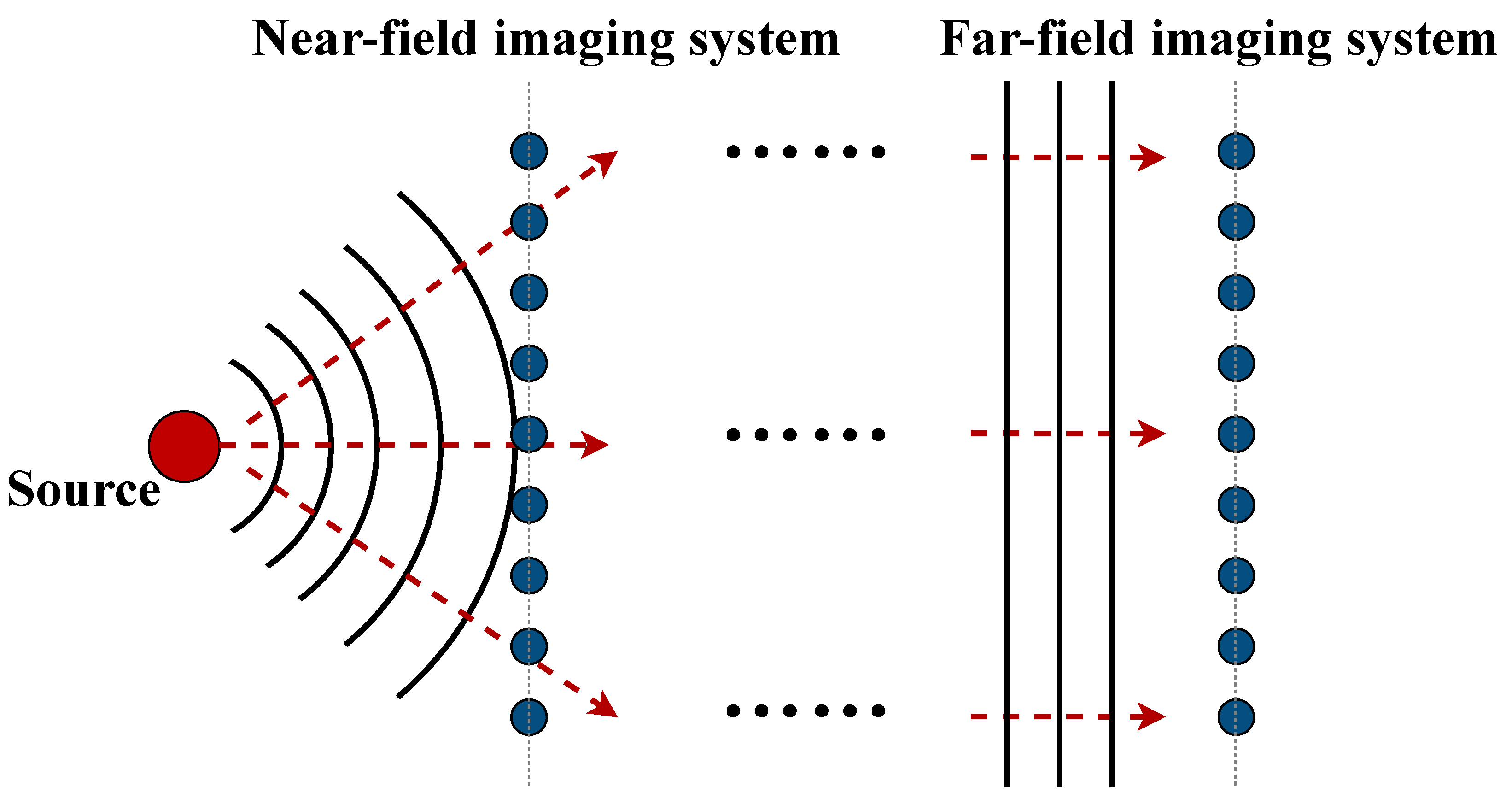
The characteristics of the target radiation signal under far- and near-field conditions are shown in
Figure 1. As illustrated in the figure, the wavefront of the target radiation signal arriving at the system array port surface is equated to a planar wavefront in the far-field condition, while it remains a spherical wavefront in the near-field condition. This difference results in the unsuitability of far-field imaging methods for near-field imaging.
Rayleigh distances [
21] in the near and far field of the SAIR imaging system are given as [
22]
The correlation function between the output signals of any two radiometer channels
i and
j in the SAIR system can be expressed completely as [
23]
where
is the Boltzmann constant;
and are the antenna directivities of each radiometer receiver channel;
and are the equivalent noise bandwidth of the receiver channel;
and are the gain of the receiver channel;
is the brightness temperature of the target scene;
is the equivalent noise temperature of the receiver channel;
and are the normalized antenna radiation pattern of each radiometer receiver channel;
is the fringe washing function between the ith and jth receiver that accounts for spatial decorrelation effects;
is the distance difference between the target to the two channels;
k is the radiometric signal wave number.
Assuming that all channels have the same antenna characteristics and channel characteristics, the correlation function can be expressed in a simplified manner, as follows:
where
and
represent the positions of the two channel.
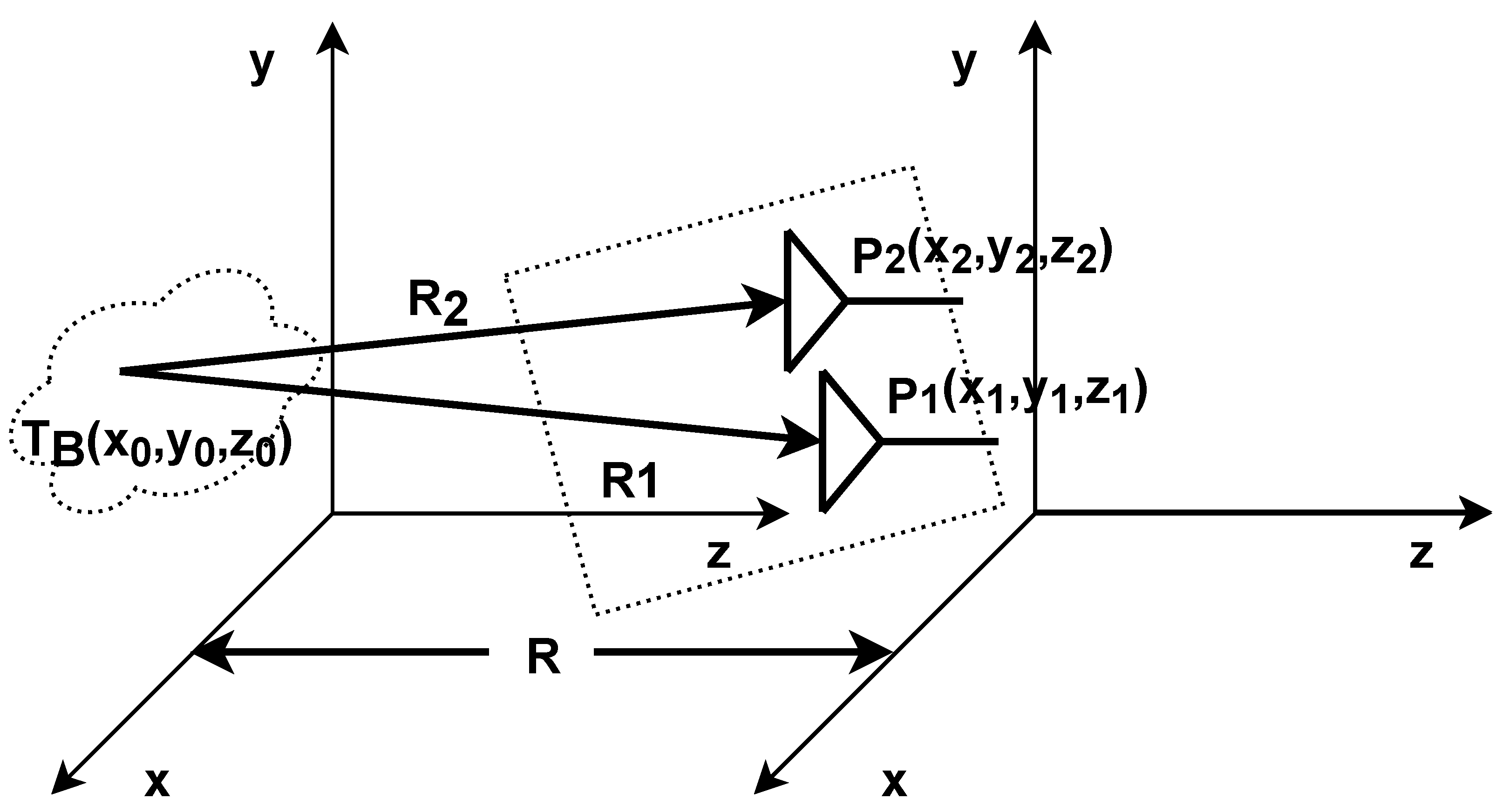
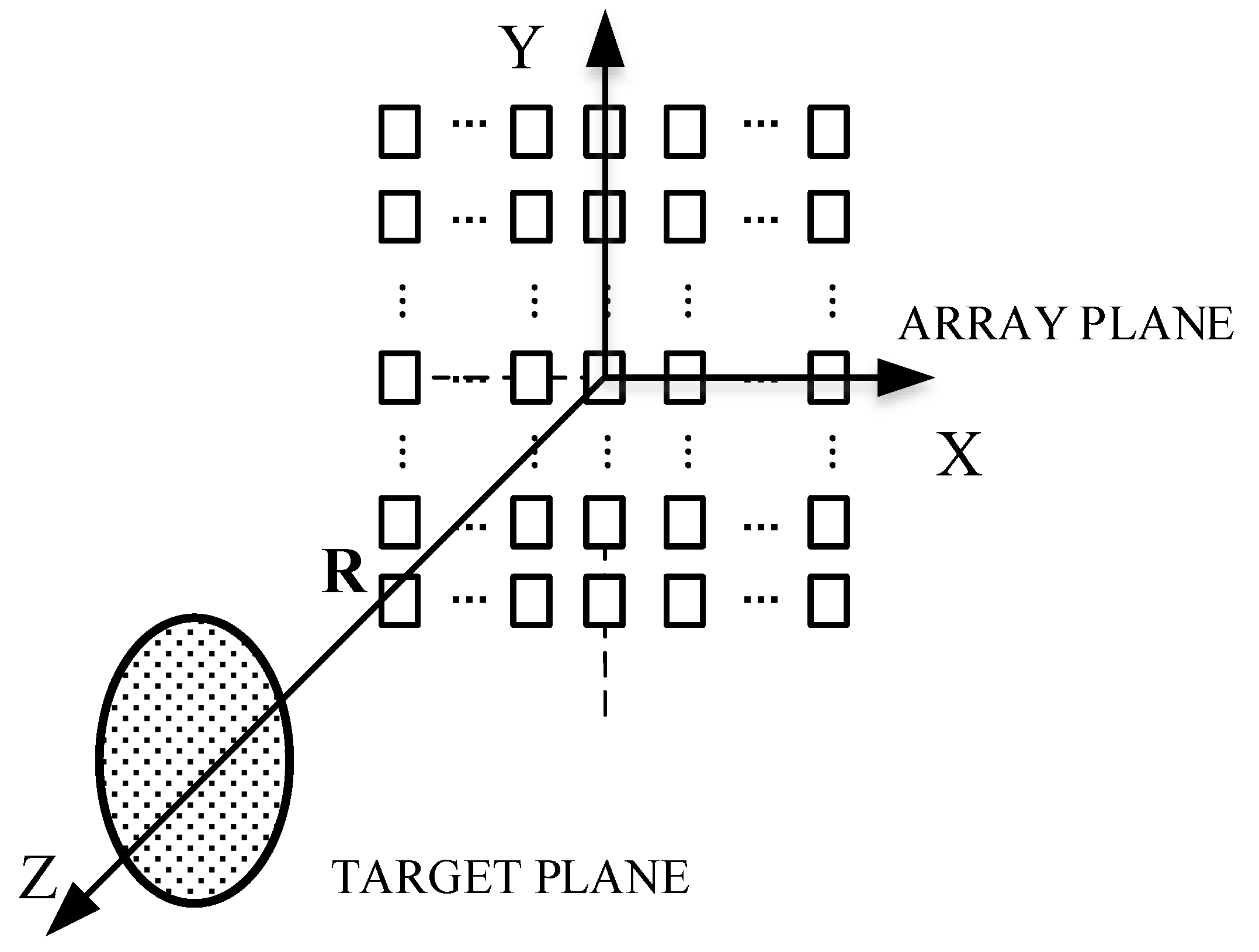
To further expand the description, a right-angle coordinate system containing the SAIR and the target is established, as shown in
Figure 2, where the coordinates of the target source
S can be expressed as
, and the coordinates of the positions of the two antennas in the imaging system are
and
.
The distance difference between the target and the two antennas can be obtained as
The distance d from the unit antenna to the origin in the far-field SAIR imaging system is smaller than the system array equivalent aperture D, whereas the distance between the target and the system R is much larger than D, so the first term in the far-field imaging can be ignored.
Under near-field conditions, only the central region of the field of view imaged by the SAIR satisfies the paraxial approximation, which is the angle between the direction of the target radiation signal, and the direction of propagation can be slight to negligible. The radiation signal from the target far from the center of the field of view does not meet the paraxial approximation when it reaches the antenna, resulting in a system error in the final imaging results. This near-field effect can be regarded as a spreading of the original image, which seriously affects the SAIR.
The presence of the near-field error term leads to aberrations in the imaging results of the inversion of the brightness temperature of the target, producing an out-of-focus effect that requires correction of the near-field visibility function to obtain the correct correlation function or the FRFT imaging method to build a mathematical model containing spherical waves. However, from another point of view, the near-field error term, although leading to the deterioration of the imaging results, also increases the amount of information, especially the distance information between the target and the array system, which is also a characteristic of near-field imaging.
We demonstrated that the signal model of the near-field SAIR can be reformulated from the fractional Fourier transform, with the following basic equation [
18]:
where
,
denotes the rotation angle of the fractional Fourier transform,
is the result of the 2D fractional Fourier transform of
,
is the transformation kernel of the 2D fractional Fourier transform, and
is the baseline and equal to the difference between the antenna positions over the
x–
y plane normalized to the wavelength.
This formula effectively achieves image reconstruction for near-field SAIR, and the distance variable is simply connected to the visibility function.
3. Proposed Distance Estimation Method for Near-Field SAIR
This section focuses on the distance estimation method for near-field SAIR. Given a specific imaging distance
, the visibility function received by the SAIR system is expressed as
. If the distance between the target and the system changes at this time, i.e., the distance is now
, the system receives the visibility function
, and the expressions of the visibility function for the two distance conditions are:
3.1. Basic Concepts of Distance Estimation Method
Using the mapping relationship between the visibility function and the target–instrument distance in the near-field SAIR, and combining the transformation relationship between the target’s bright temperature and the near-field visibility function, the target–instrument distance estimation method applicable to the near-field SAIR system is derived.
First, in the
plane, the Fourier transform of the visibility function
is
where
denotes the high-level visibility function. Considering the propagation direction
of the radiation signal and defining its directional angle as
, this radiation signal can be expressed as
where
is the position vector (the symbol
denotes the unit vector), and
. Therefore, in the plane where
z is a constant, the radiation signal amplitude can be expressed as
The complex exponential function
can be regarded as a plane wave in the plane of
; then, the corresponding propagation direction can be expressed as
In the Fourier decomposition of the visibility function
V, the corresponding spatial frequency is
, and the corresponding complex amplitude is
, which leads to
is the Fourier transform of the visibility function
, that is,
Then, the visibility function
can be written as
By the nature of the visibility function [
23], it is known that
needs to satisfy
The solution of (
14) can be expressed as
Inverting the above equation and bringing in (
7) yields
The above equation shows that under near-field conditions, the visibility functions at different distances can be related by Equation (
16).
According to the derivation of the formula in the previous section, the near-field visibility function at different distances can be obtained by changing the spacing between the target and the SAIR array. Using the above formula, the initial target’s distance can be derived by taking into account the near-field visibility function at different distances and the corresponding spacing.
3.2. Iterative Distance Estimation Method
The method described above can obtain the target–instrument distance, but it requires manual adjustment of the parameters to obtain the near-field imaging results using step-by-step attempts and does not guarantee the optimal imaging quality in the final results. Therefore, an optimization algorithm was designed to combine the near-field imaging distance analysis with the rotation parameters in the fractional-order Fourier transform. This allows for the acquisition of the near-field imaging results with an unknown target–instrument distance by adjusting the rotation parameters. The imaging quality is evaluated and constraints are given for further adjustment until the optimal imaging result is achieved. The imaging distance under these conditions is considered the real target–instrument distance.
A corresponding mathematical model was developed to investigate the influence of the target–instrument distance on the quality of the final imaging results under the premise that the target scene and the target–instrument distance are unknown and that the visibility function and the array arrangement of the near-field SAIR imaging system and the corresponding system parameters are known. In the process of using the near-field fractional-order imaging method, the inversion of the near-field visibility function is performed at different target–instrument distances to obtain the imaging results. The quality of the image at each target–instrument distance is evaluated to obtain the optimal imaging result.
In simulation scenarios where the original image information is known, the root mean square error (RMSE) can be well employed to assess the imaging quality. However, under most real conditions, the brightness temperature distribution of the original image is not available. Therefore, it is impossible to compare the brightness temperature of the near-field imaging image with the brightness temperature distribution of the original image to obtain the root mean square error of the imaging results. The reference-free inverse image evaluation index is needed to break away from the dependence on the ideal reference image.
Near-field imaging results are characterized by blurring and image spreading due to the spherical wave of the target radiation signal; thus, high-resolution and clear images can be used as the basis for evaluating imaging results. In the absence of the original image, the average gradient [
24] can be employed as a criterion for assessment because it is a measure of the image’s clarity. The definition of average gradient (AG) is
where
denotes the image brightness temperature;
denotes the number of pixels in the horizontal and vertical directions of the image, respectively. The larger the average gradient calculated according to the above equation, the greater the image detail and the higher the sharpness.
Considering that the imaging results of the SAIR system are noise-related, the metrics should be adjusted to include the overall noise level of the image. The definition of the modified average gradient (MAG) when image quality assessment is
where
is the variance of the inversion image. The MAG value can be calculated to compare and judge the accuracy of the estimated estimation.
According to the previous analysis, it is known that the closer the actual distance, the better the quality of the image. Therefore, an optimization algorithm can be employed to determine the target–instrument distance. In this study, the simulated annealing algorithm [
25] was chosen to solve the actual imaging distance of the target due to its ability to find the global optimal solution with a higher probability. The optimization parameters used for assessing the image quality in the algorithm are thoroughly analyzed in the following subsection.
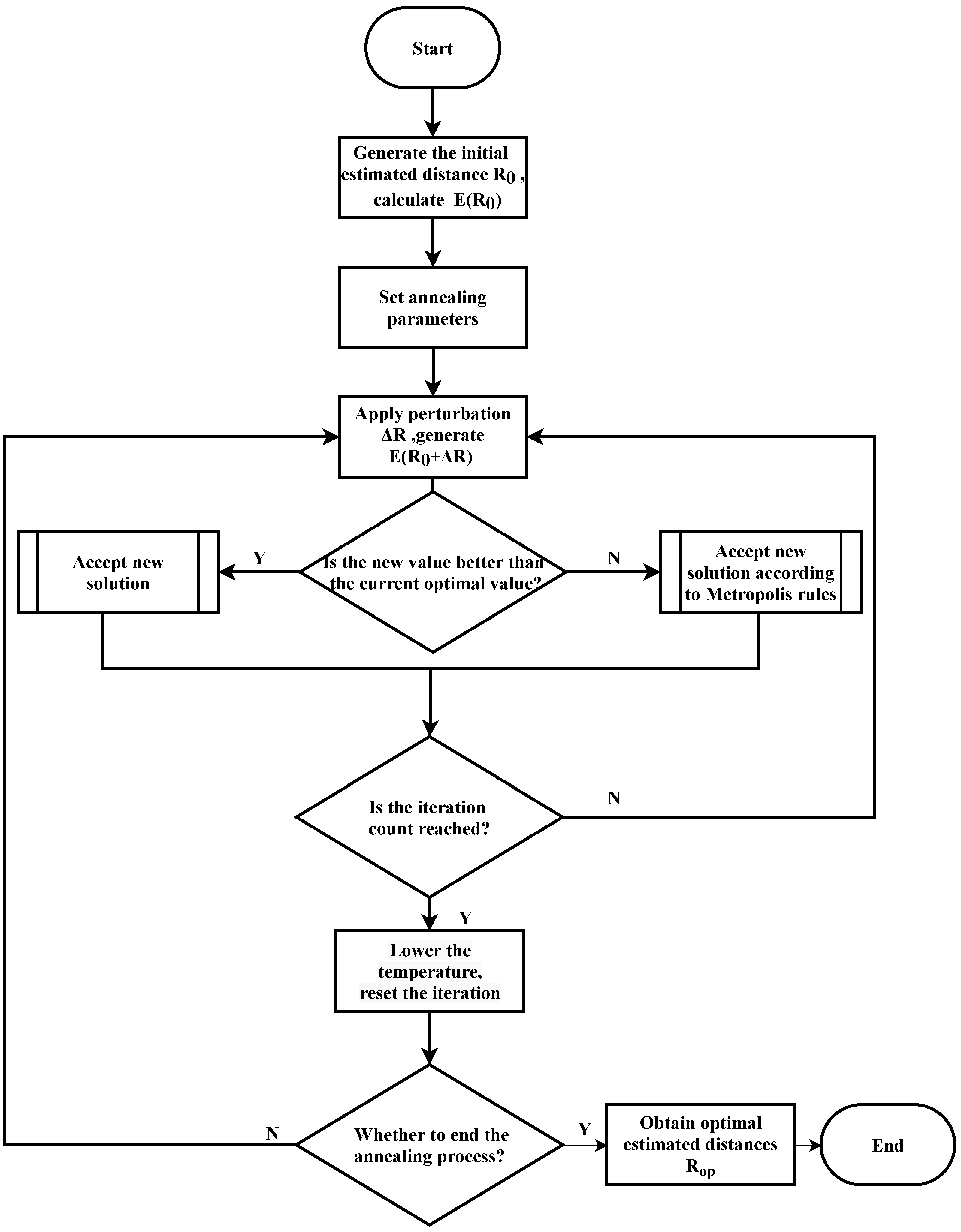
The steps for solving the target–instrument distance using the simulated annealing algorithm can be written as
Initialize at an initial annealing temperature and generating a random initial solution as the initial solution and calculating the corresponding objective function . The initial solution represents the initial target–instrument distance , and the corresponding objective function is the reciprocal of MAG.
Set the cooling rate for this temperature.
Apply a random perturbation to the current target–instrument distance
to generate a new solution
in the current domain and calculate the corresponding objective function
.
According to the Metropolis criterion, the distance
can be received as the current solution or does not need to be calculated according to the following probabilities.
Repeat steps 2, 3, and 4 above until the equilibrium at the current temperature is reached.
Lower the temperature and repeat the iterative process.
Determine if the temperature reaches the termination temperature; if yes, then terminate the algorithm; otherwise, return to step 2.
The flowchart of the simulated annealing algorithm for the target–instrument distance estimation optimization problem is shown in
Figure 3.
In the iterative process, the target–instrument distance
R is the solution
x. The selection of the cooling scheme is a crucial step in the simulated annealing algorithm, and based on the near-field imaging distance characteristics, we propose using an exponential approach for cooling.
where
is the initial temperature of the algorithm, and the parameter
denotes the annealing factor, which generally has a
.
As the iteration temperature cools in the target–instrument distance optimization problem based on the simulated annealing algorithm, the inverse image quality gradually improves. When the iteration temperature reaches the algorithm’s minimum temperature , the micromovement of the target–instrument distance can no longer improve the quality of the inverse image, and the global optimal solution is reached. The optimal estimated target–instrument distance is also obtained.
4. Experimental Analysis
In this section, the performance of the proposed method is verified by numerical simulations and real experiments.
4.1. One-Dimensional Imaging
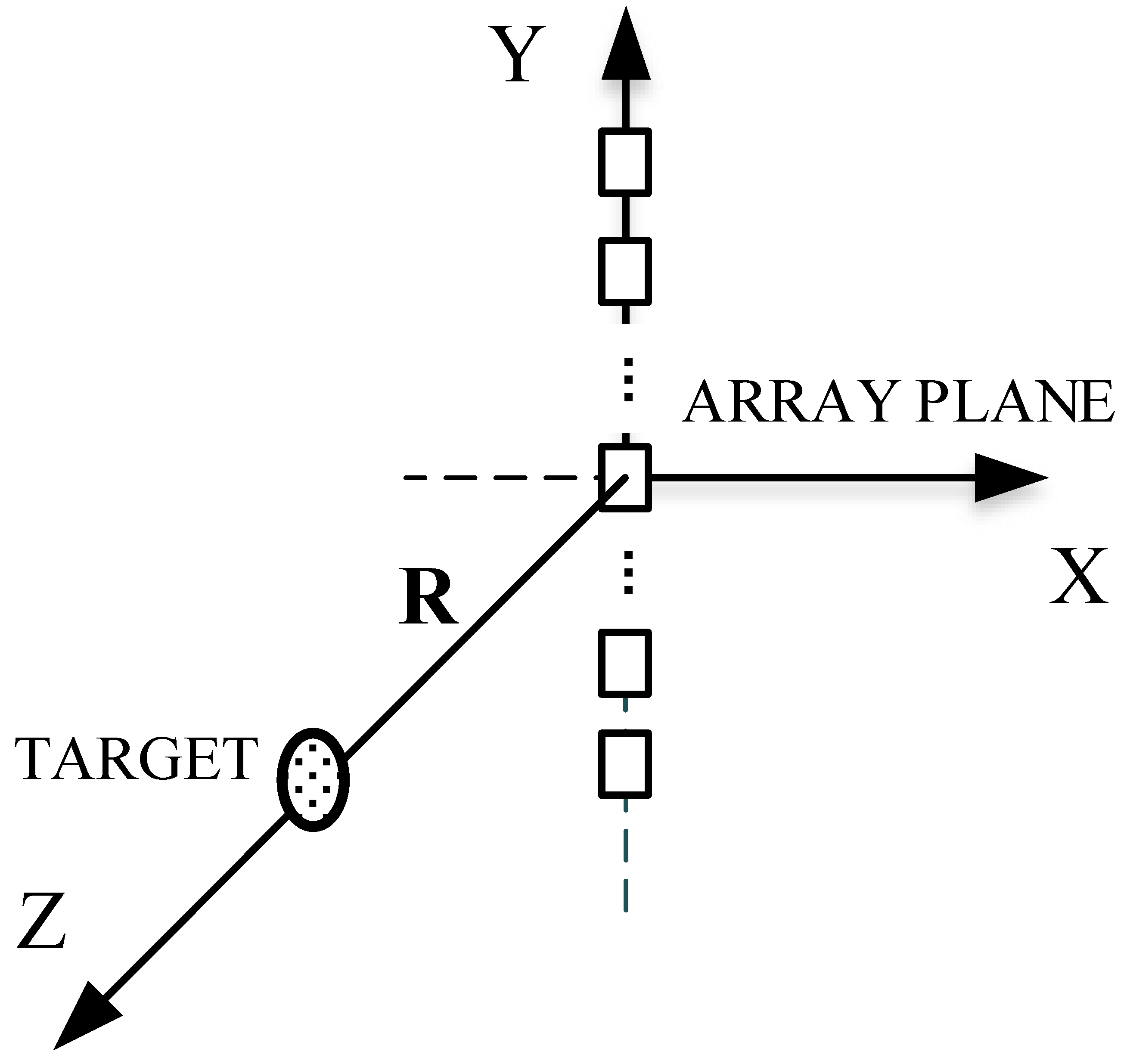
The first simulation array is a homogeneous one-dimensional line array consisting of 25 channels for simulated experimental imaging of a point target at a distance of 1 m. The schematic diagram of the target and the one-dimensional line array are shown in
Figure 4.
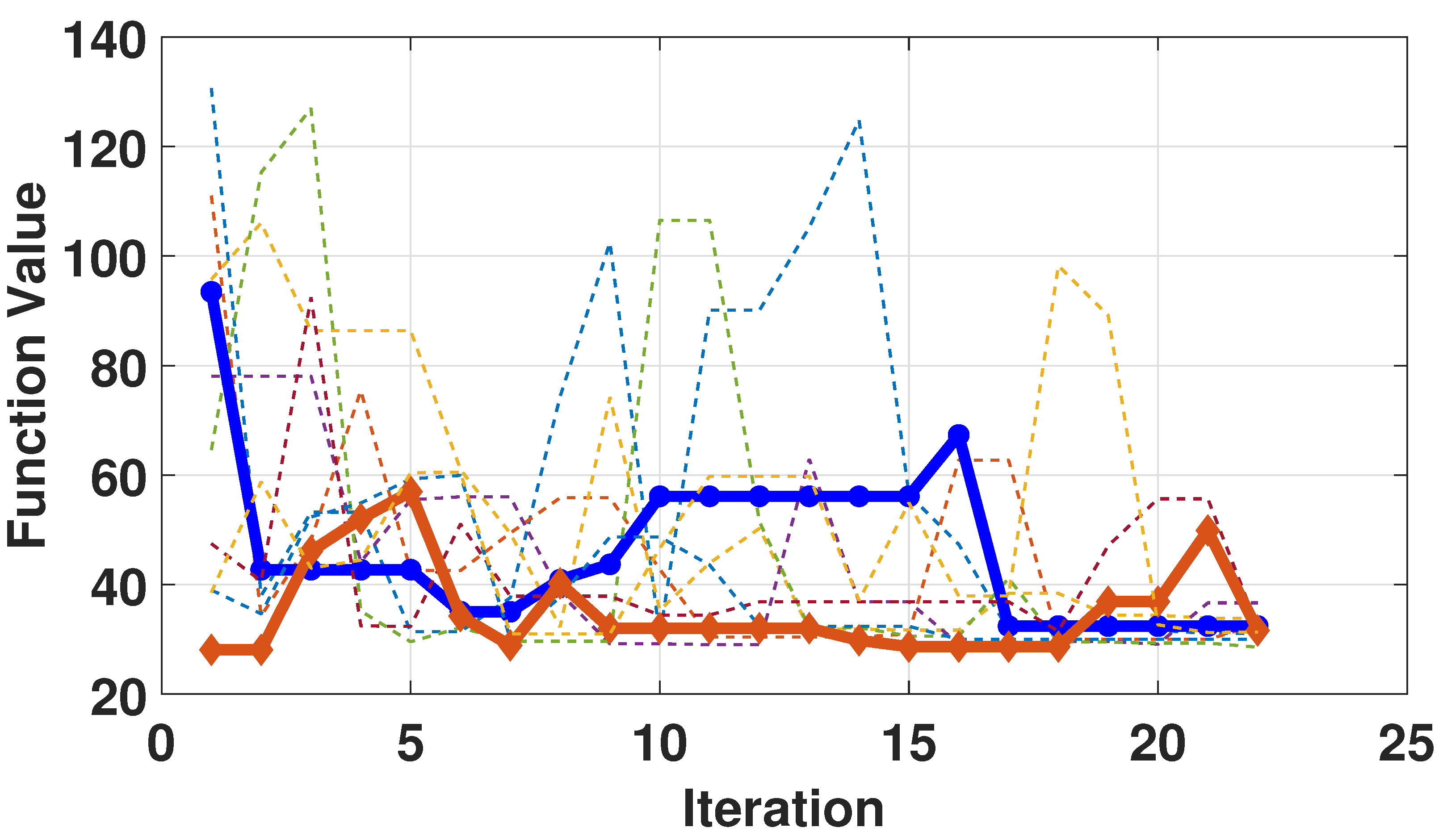
An imaging system with one-dimensional linear array structure was used to simulate imaging experiments on targets at unknown distances using the distance estimation method proposed in this paper. The iteration curve of the algorithm is shown in
Figure 5. Based on multiple experimental experiences and final results, we found that setting the iteration process to around 20 times could achieve a relatively accurate estimation of distance, and further increasing the iteration time did not significantly improve the estimation accuracy. Each curve in
Figure 5 represents a different iteration process with a different initial estimation value. From the convergence results of all the curves, it can be seen that an accurate estimation distance could be obtained regardless of the initial estimation distance, which was very close to the true target–instrument distance. The red curve with rectangular marker in
Figure 5 represents the iteration curve with an initial value of 1 m, and it can be seen that the optimal function value of this curve is the initial value.
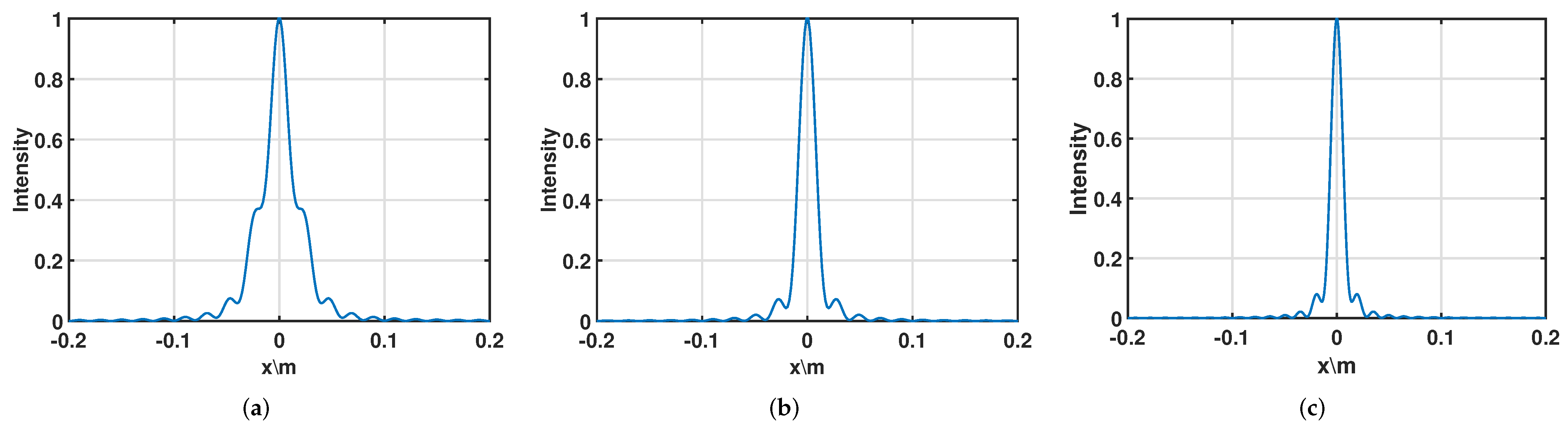
Figure 6 shows the imaging results during one of the iteration processes, corresponding to the blue curve with circular marker in
Figure 5. The optimal estimated distance obtained at the end of this iteration process was 1.086 m. All images were normalized to make them more straightforward to contrast the imaging results. Three imaging results during the iteration processes are provided in
Table 1. It was discovered that the imaging outcomes and MAG both steadily improved when the estimated distance was close to the actual target–instrument distance. The result confirms the viability of the method used in this study to estimate the distance.
The optimal estimated distance obtained from each iteration in
Figure 5 were plotted in a table, as shown in
Table 2. It can be seen from the table that the final estimated distances obtained from each iteration were very close to the actual target distance of 1 m, regardless of the initial distance set for the iteration, which also demonstrates the effectiveness of the proposed near-field imaging distance estimation method proposed in this paper.
From
Table 2, it can be concluded that regardless of how the initial value of the estimation method is set, a relatively accurate estimate of the target–instrument distance can be obtained after 20 iterations. The mean square error (MSE) was used to evaluate the error of the distance estimation method, and the specific calculation formula is as follows:
where
N is the number of estimated distances,
is the
ith optimal estimated distance, and
is the real target–instrument distance. The MSE of this near-field target–instrument distance estimation method under the one-dimensional array condition could be calculated as
.
4.2. Two-Dimensional Imaging
After the analysis of the 1D array imaging system, research and simulation of the 2D imaging system were further carried out. This simulation-based experimental system array layout is shown in
Figure 7, which we used to avoid the influence of system sparsity. The array element spacing was
for a rectangular full array with a total of
array elements. The distance between the set scene and the array was 1 m.
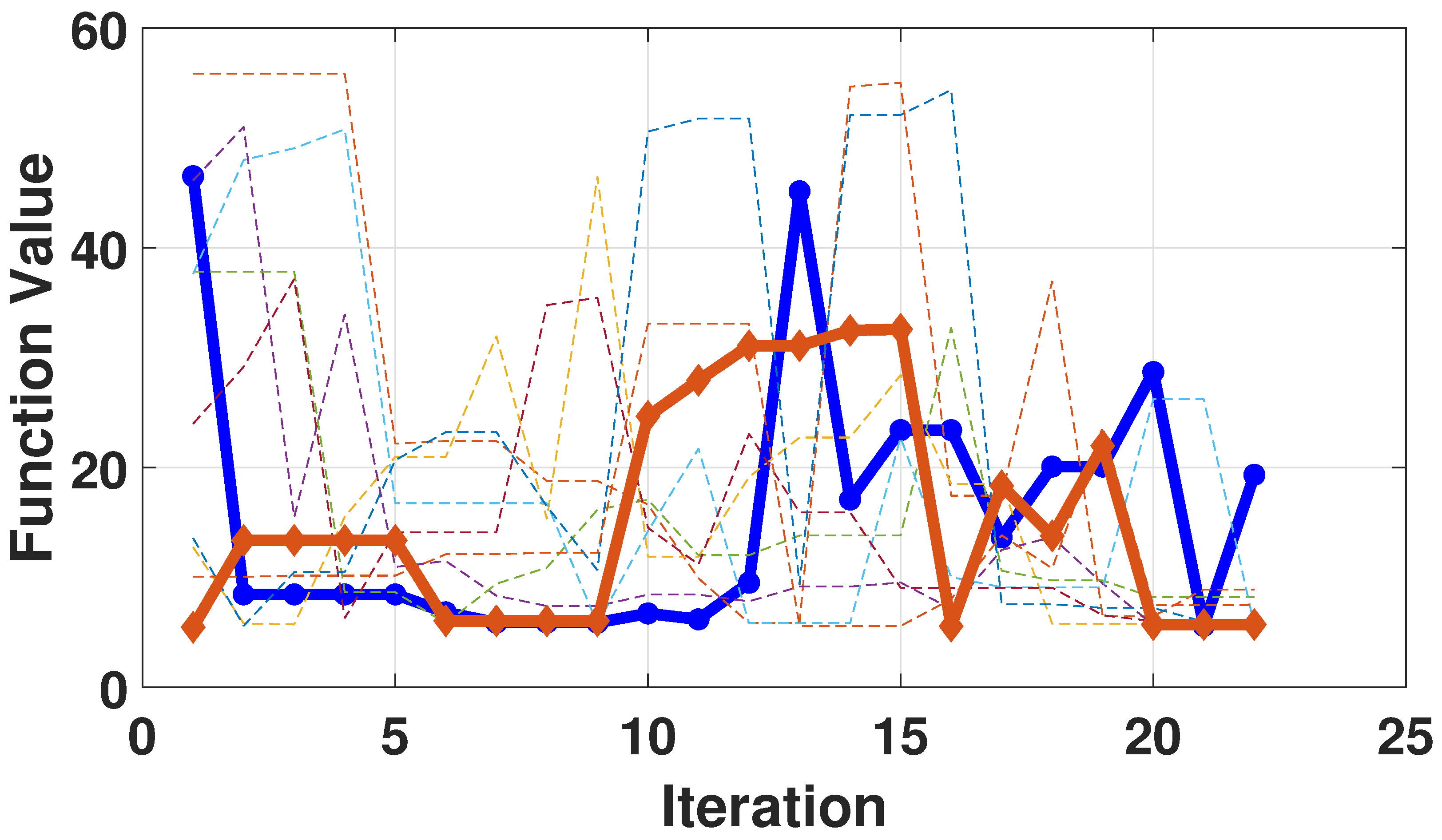
Using the target–instrument distance estimation method based on the simulated annealing algorithm, the objective function was set as the reciprocal of MAG, and the objective function convergence curves were obtained as shown in
Figure 8 by reasonably setting the initial temperature, the cooling rate, and the end condition in the simulated annealing algorithm. Again, within 20 iterations, each curve provided accurate distance estimates. The iteration curve with an initial value of 1 m is represented by the red curve with a rectangular-marker in
Figure 8, and it can be noticed that the optimal function value of this curve is the initial value.
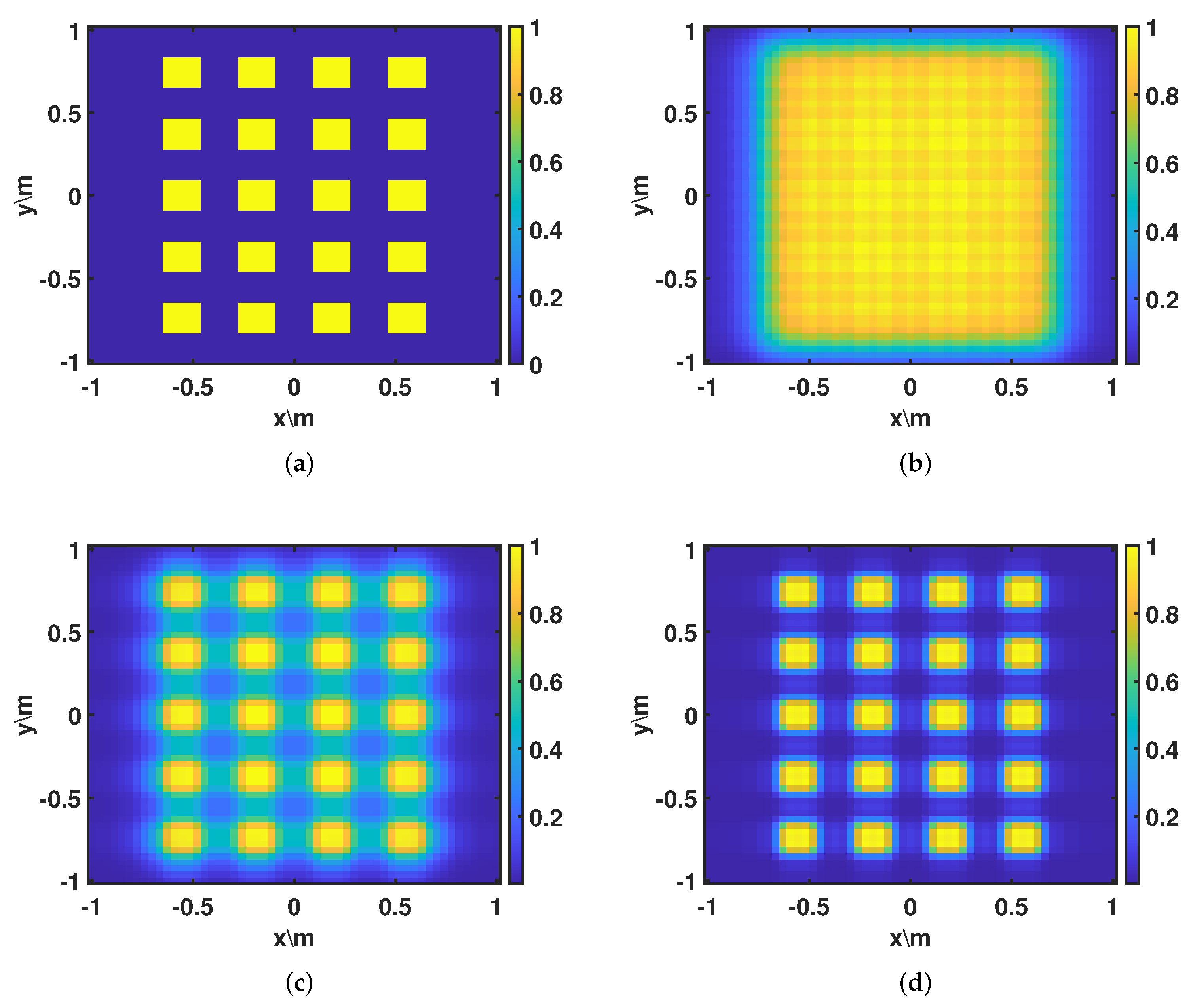
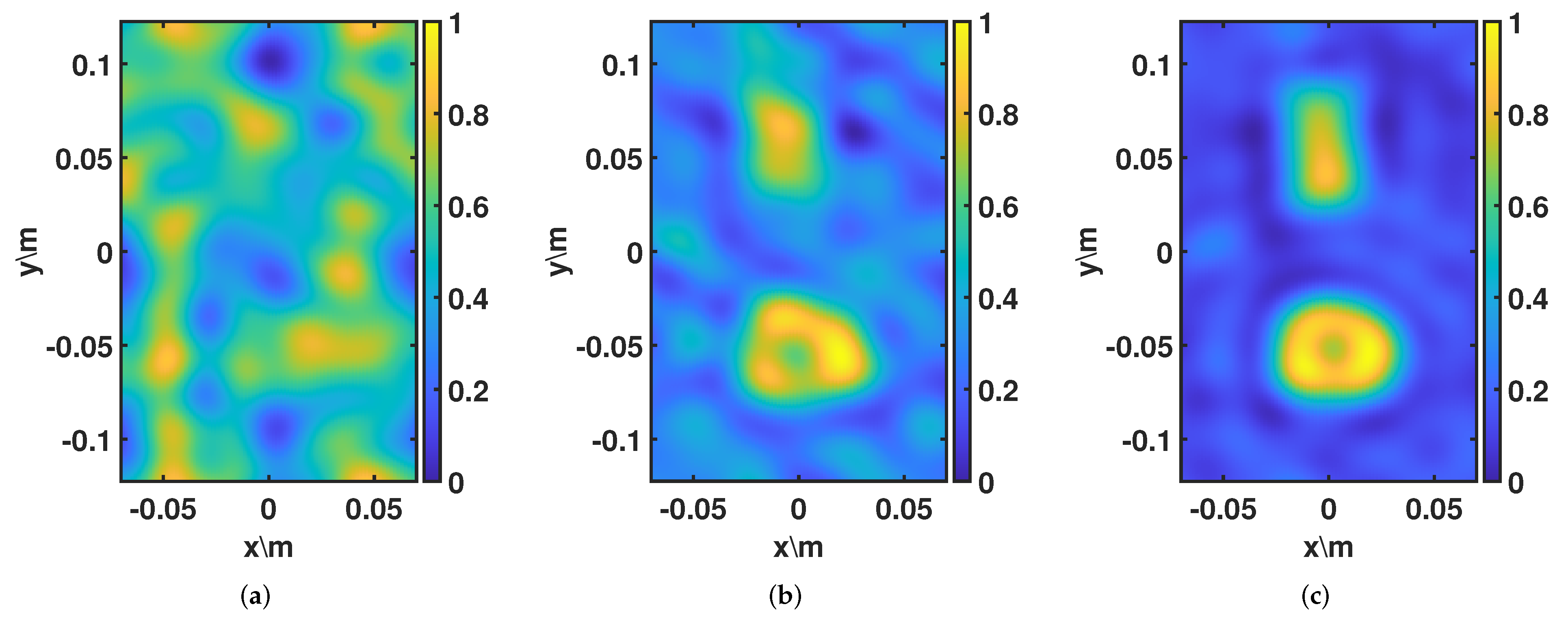
Figure 9 shows three imaging results during one of the iteration processes, corresponding to the blue curve with a circular marker in
Figure 8. The estimated distance obtained at the end of this iteration process was 1.012 m, which is basically the same as the actual distance. This result verifies the effectiveness of the target–instrument distance prediction method based on the simulated annealing algorithm. The three imaging results during the iteration processes are shown in
Table 3. It was discovered that both the imaging results and the calculated data steadily improved when the estimated distance was close to the actual target–instrument distance. This result confirms the viability of the distance estimation method used in this study.
As already mentioned, if the real bright temperature of the target is known, the RMSE can be used to evaluate the imaging results. The RMSE of the inverse image at different estimated distances in
Figure 9 was calculated. From
Table 3, it can be seen that as the distance was iterated and approximated to the real value, the RMSE of the final imaging results reached 0.1299, and the image quality was close to the ideal result, which demonstrates that MAG can be used as a metric to evaluate distance estimation when the real image is unknown.
The optimal estimated distance that was derived with each iteration in
Figure 8 is displayed in
Table 4. The validity of the near-field imaging distance estimation method suggested in this paper is further demonstrated by the table, which shows that the final estimated distances acquired from each iteration were extremely close to the real target distance.
The MSE of this near-field target–instrument distance estimation method under the two-dimensional array condition was calculated as 0.0011. It was not unusual that this result differed from that of the 1D array imaging system, as there were variations in the array layout structure, different target types, etc.
4.3. Real Measurement Imaging Experiment
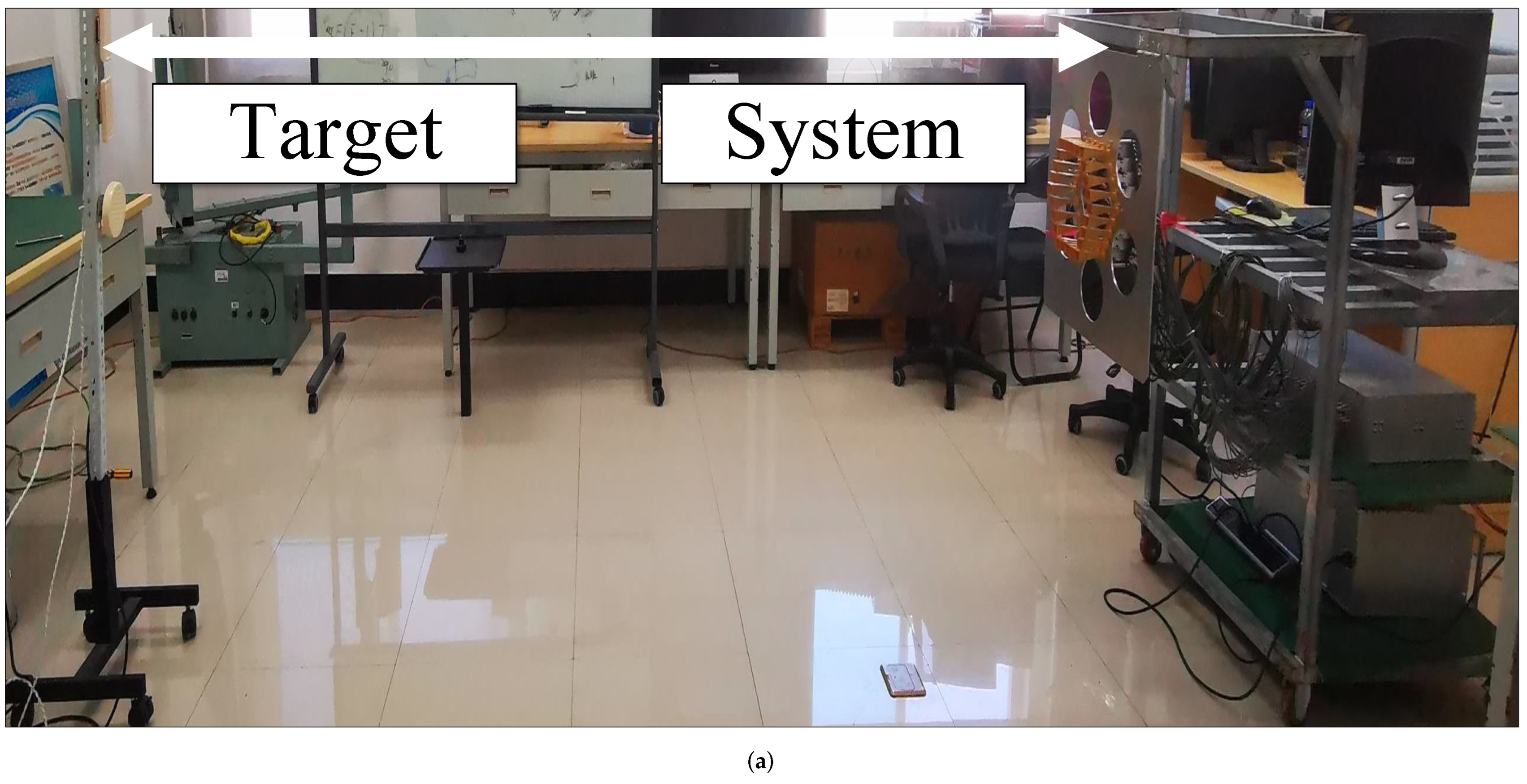
A high-performance system was constructed to further confirm the viability of the distance estimate approach for real applications. As shown in
Figure 10, the near-field radiometer experimental system consisted of a 24 antenna array, RF channels, and a subsequent high-speed digital processing center. The center frequency was 94 GHz, and the bandwidth was 400 MHz. The distance between the real extended source and the near-field SAIR imaging system was set at 2 m.
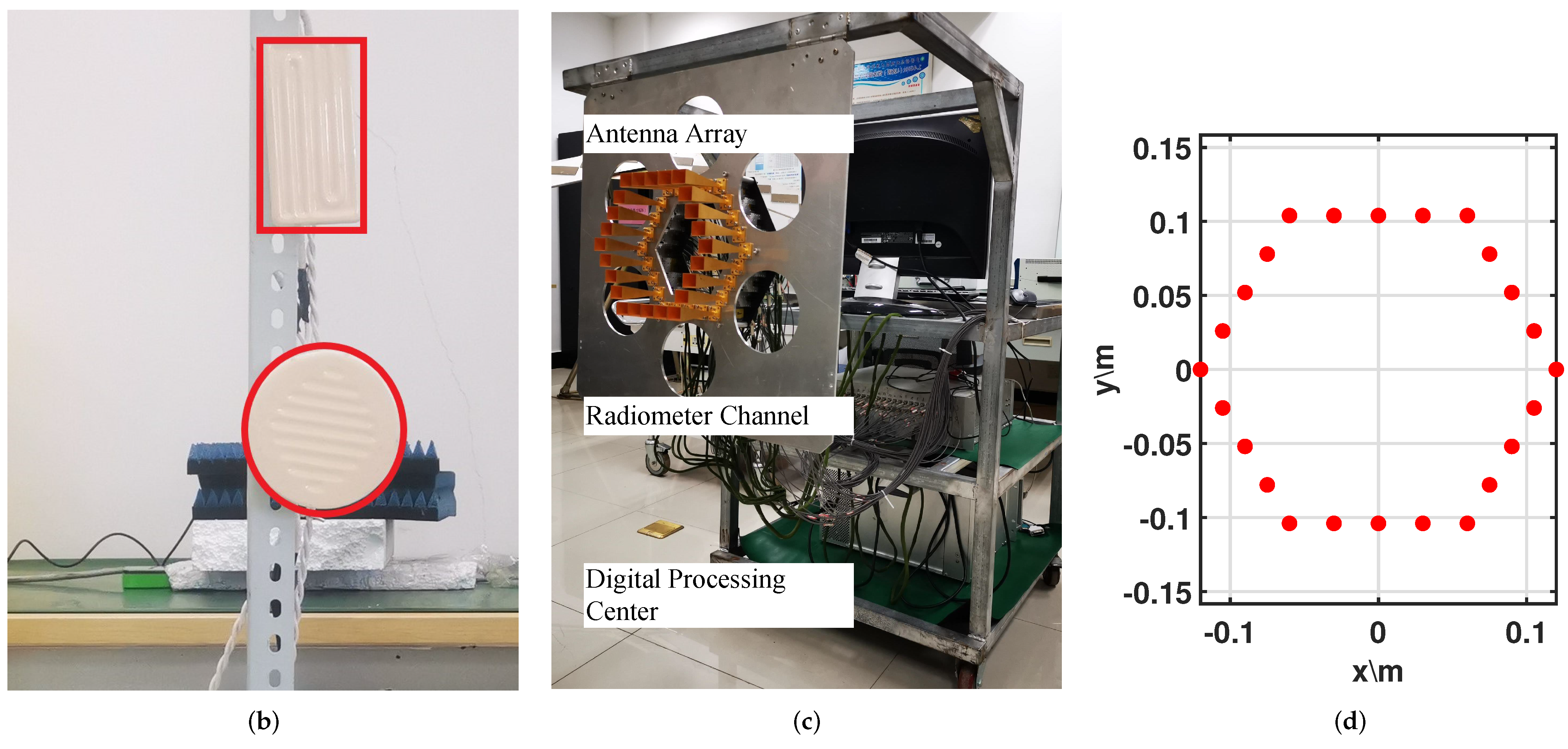
The analysis for the real near-field imaging system was similar to that described in the previous section, the objective function was set as the reciprocal of MAG, and the objective function convergence curve was obtained as shown in
Figure 11 by reasonably setting the initial temperature, the cooling rate, and the end condition in the simulated annealing algorithm.
The blue circular marked curve in
Figure 11 was chosen to demonstrate the effectiveness of the estimated method. The optimal estimated distance obtained in this iteration process was 1.9488 m, which was very close to the true value. The three imaging results in
Figure 12 represent the three results of this iteration process.
The MAG and corresponding estimated distances for this iteration process can be found in
Table 5. From the graphical results and the iterative process, it can be revealed that the distance estimation algorithm proposed in this paper can satisfactorily estimate the target–instrument distance of the real imaging system and thus obtain accurate imaging results.
Finally, the initial estimated distance values and the optimal estimated distances for all iterative processes in
Figure 11 are likewise given in
Table 6. Further calculations yielded an MSE of 0.0083 for the near-field target–instrument distance estimation algorithm applied to this real imaging system.
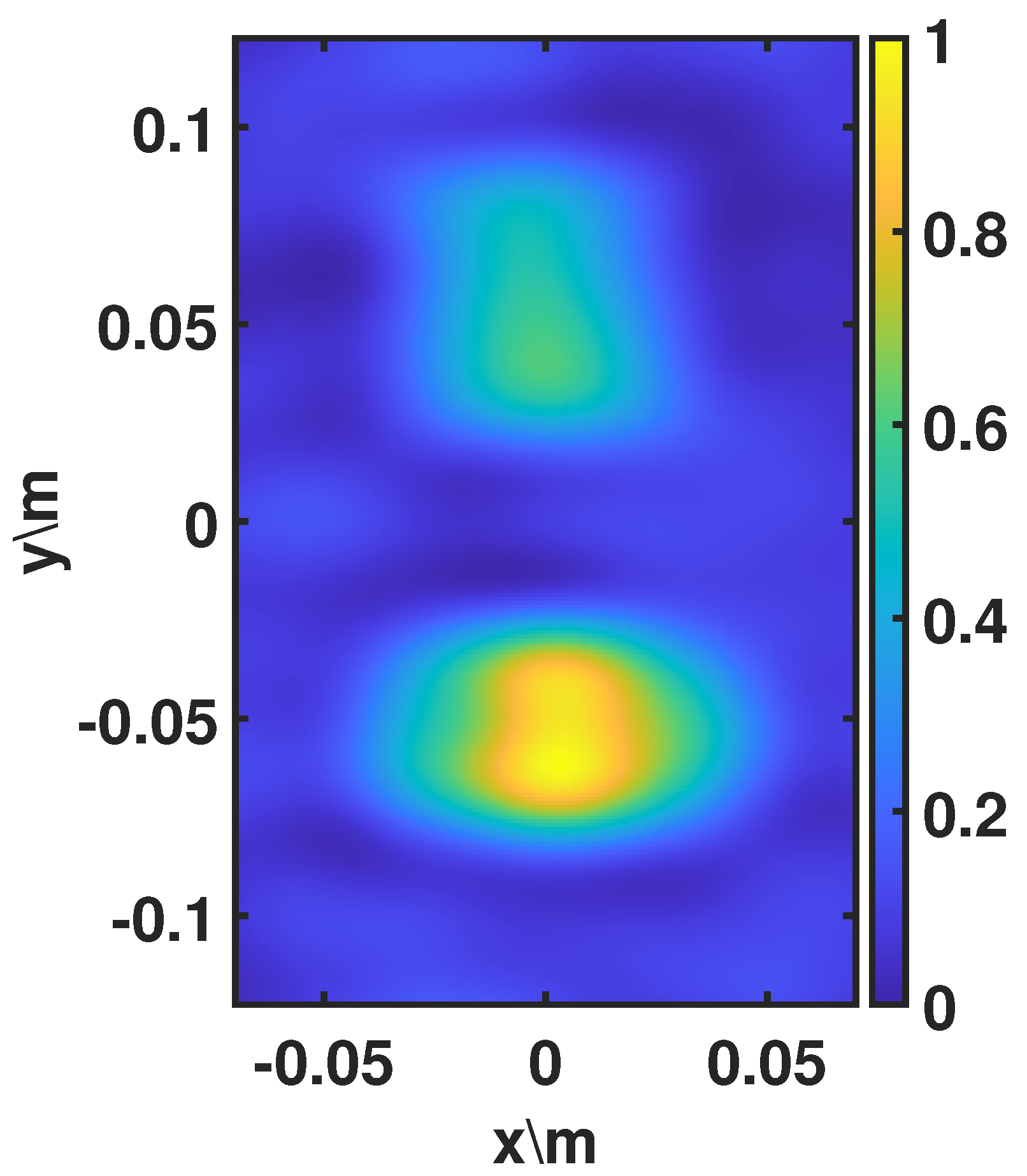
Although there are no other comparable methods for estimating near-field target–instrument distance at present, we used a far-field imaging method (synthetic aperture radiometry) to directly image near-field targets, as shown in
Figure 13. The MAG of this result was 0.1069. It was observed that target–instrument distance is crucial for synthetic aperture radiometer near-field imaging, and our method can accurately estimate the distance and obtain high-quality imaging results.
5. Conclusions
In this study, the information contained in the visibility function under far-field conditions as well as near-field conditions was first investigated, and it was found that the distance information of the target can be recovered from the near-field visibility function. To this end, we developed a novel near-field target–instrument distance estimation method that can iteratively derive the distance between the target and the system when the target–instrument distance is unknown. The simulated annealing algorithm was employed in the iteration of distance estimation, and the MAG parameter was also proposed as the optimization objective in order to effectively evaluate the iterative process. The optimal solution for the target–instrument distance was finally obtained iteratively with the Metropolis criterion. Then high-quality imaging results of the target were obtained by the fractional Fourier method. Numerical simulation and real experiments were carried out to demonstrate the validity and effectiveness of the proposed distance estimation method for near-field SAIR imaging systems. Moreover, several experiments were performed by varying the initial estimated distance, and the MSE of the distance estimation method was calculated for different array structures. Our results indicated that a relatively accurate estimated distance could be obtained in about 20 iterations, which required no more than 30 s based on the capabilities of the existing PC. Therefore, we think that this distance estimation method has good prospects for future applications.
In future research, the accuracy and speed of the distance estimation method will be further improved. It is possible to incorporate prior scene information into the iterative process to reduce the number of iterations and quickly obtain the target–instrument distance. Additionally, we will separately investigate the relationship between the distance accuracy and the system array arrangement, as well as other performance parameters, in subsequent research. Overall, we think that the proposed distance estimation method has great potential for practical applications in near-field SAIR imaging systems, and we will continue to explore ways to optimize its performance.
Author Contributions
Conceptualization, H.H. and F.H.; data curation, H.H.; formal analysis, H.H. and D.Z.; funding acquisition, D.Z. and F.H.; methodology, H.H. and D.Z.; project administration, H.H.; resources, H.H. and F.H.; supervision, F.H.; validation, H.H. and D.Z.; writing—original draft, H.H.; writing—review and editing, H.H., D.Z. and F.H. All authors have read and agreed to the published version of the manuscript.
Funding
This work was supported in part by National Natural Science Foundation of China under grant 62271219, grant 61901244, and grant 61871438; and in part by the Fundamental Research Funds for the Central Universities (Huazhong University of Science and Technology).
Data Availability Statement
Not applicable.
Conflicts of Interest
The authors declare no conflict of interest.
References
- Ruf, C.S.; Swift, C.T.; Tanner, A.B.; Le Vine, D.M. Interferometric synthetic aperture microwave radiometry for the remote sensing of the Earth. IEEE Trans. Geosci. Remote Sens. 1988, 26, 597–611. [Google Scholar] [CrossRef]
- Le Vine, D.M. Synthetic aperture radiometer systems. IEEE Trans. Microw. Theory Tech. 1999, 47, 2228–2236. [Google Scholar] [CrossRef]
- Anterrieu, E.; Waldteufel, P.; Lannes, A. Apodization functions for 2-D hexagonally sampled synthetic aperture imaging radiometers. IEEE Trans. Geosci. Remote Sens. 2002, 40, 2531–2542. [Google Scholar] [CrossRef]
- Corbella, I.; Duffo, N.; Vall-Llossera, M.; Camps, A.; Torres, F. The visibility function in interferometric aperture synthesis radiometry. IEEE Trans. Geosci. Remote Sens. 2004, 42, 1677–1682. [Google Scholar] [CrossRef]
- Martín-Neira, M.; LeVine, D.; Kerr, Y.; Skou, N.; Peichl, M.; Camps, A.; Corbella, I.; Hallikainen, M.; Font, J.; Wu, J. Microwave interferometric radiometry in remote sensing: An invited historical review. Radio Sci. 2014, 49, 415–449. [Google Scholar] [CrossRef]
- Bosch-Lluis, X.; Reising, S.C.; Kangaslahti, P.; Tanner, A.B.; Brown, S.T.; Padmanabhan, S.; Parashare, C.; Montes, O.; Razavi, B.; Hadel, V.D.; et al. Instrument design and performance of the high-frequency airborne microwave and millimeter-wave radiometer. IEEE J. Sel. Topics Appl. Earth Observ. Remote Sens. 2019, 12, 4563–4577. [Google Scholar] [CrossRef]
- Zhu, D.; Lu, H.; Cheng, Y. RFI source detection based on reweighted ℓ1-norm minimization for microwave interferometric radiometry. IEEE Trans. Geosci. Remote Sens. 2021, 60, 1–15. [Google Scholar]
- Zhu, D.; Tao, J.; Xu, Y.; Cheng, Y.; Lu, H.; Hu, F. RFI localization via reweighted nuclear norm minimization in microwave interferometric radiometry. IEEE Trans. Geosci. Remote Sens. 2022, 60, 1–17. [Google Scholar] [CrossRef]
- Lu, H.; Li, Y.; Li, H.; Lv, R.; Lang, L.; Li, Q.; Song, G.; Li, P.; Wang, K.; Xue, L. Ship detection by an airborne passive interferometric microwave sensor (PIMS). IEEE Trans. Geosci. Remote Sens. 2019, 58, 2682–2694. [Google Scholar] [CrossRef]
- Salmon, N.A. Outdoor passive millimeter-wave imaging: Phenomenology and scene simulation. IEEE Trans. Antennas Propag. 2017, 66, 897–908. [Google Scholar] [CrossRef]
- Salmon, N.A. Indoor full-body security screening: Radiometric microwave imaging phenomenology and polarimetric scene simulation. IEEE Access 2020, 8, 144621–144637. [Google Scholar] [CrossRef]
- Peichl, M.; Suess, H.; Suess, M.; Kern, S. Microwave imaging of the brightness temperature distribution of extended areas in the near and far field using two-dimensional aperture synthesis with high spatial resolution. Radio Sci. 1998, 33, 781–801. [Google Scholar] [CrossRef]
- Tanner, A.B.; Lambrigsten, B.H.; Gaier, T.M.; Torres, F. Near field characterization of the GeoSTAR demonstrator. In Proceedings of the IEEE IGARSS, Denver, CO, USA, 31 July–4 August 2006; pp. 2529–2532. [Google Scholar]
- Tanner, A.B.; Swift, C.T. Calibration of a synthetic aperture radiometer. IEEE Trans. Geosci. Remote Sens. 1993, 31, 257–267. [Google Scholar] [CrossRef]
- Laursen, B.; Skou, N. Synthetic aperture radiometry evaluated by a two-channel demonstration model. IEEE Trans. Geosci. Remote Sens. 1998, 36, 822–832. [Google Scholar] [CrossRef] [Green Version]
- Bosch-Lluis, X.; Ramos-Perez, I.; Camps, A.; Rodriguez-Alvarez, N.; Valencia, E.; Park, H. Common mathematical framework for real and synthetic aperture by interferometry radiometers. IEEE Trans. Geosci. Remote Sens. 2014, 52, 38–50. [Google Scholar] [CrossRef]
- Li, J.; Hu, F.; He, F.; Wu, L. High-resolution RFI localization using covariance matrix augmentation in synthetic aperture interferometric radiometry. IEEE Trans. Geosci. Remote Sens. 2018, 56, 1186–1198. [Google Scholar] [CrossRef]
- Hu, H.; Zhu, D.; Hu, F. A novel imaging method using fractional Fourier transform for near-field synthetic aperture radiometer systems. IEEE Geosci. Remote Sens. Lett. 2022, 19, 1–5. [Google Scholar] [CrossRef]
- Kumar, L.; Hegde, R.M. near-field acoustic source localization and beamforming in spherical harmonics domain. IEEE Trans. Signal Process. 2016, 64, 3351–3361. [Google Scholar] [CrossRef]
- Wang, Y.; Ho, K.C. Unified near-field and far-field localization for AOA and hybrid AOA-TDOA positionings. IEEE Trans. Wirel. Commun. 2018, 17, 1242–1254. [Google Scholar] [CrossRef]
- Nova, E.; Romeu, J.; Torres, F.; Pablos, M.; Riera, J.M.; Broquetas, A.; Jofre, L. Radiometric and spatial resolution constraints in millimeter-wave close-range passive screener systems. IEEE Trans. Geosci. Remote Sens. 2013, 51, 2327–2336. [Google Scholar] [CrossRef]
- Salmon, N.A. Near-field aperture synthesis millimeter wave imaging for security screening of personnel. In Proceedings of the 9th International Symposium on Communication Systems, Networks and Digital Signal Processing, Manchester, UK, 23–25 July 2014; pp. 1082–1085. [Google Scholar]
- Camps Carmona, A.J. Application of Interferometric Radiometry to Earth Observation. Ph.D. Thesis, Universitat Politècnica de Catalunya, Catalonia, Spain, 1996. [Google Scholar]
- Li, W.; Hu, X.; Du, J.; Xiao, B. Adaptive remote-sensing image fusion based on dynamic gradient sparse and average gradient difference. Int. J. Remote Sens. 2017, 38, 7316–7332. [Google Scholar] [CrossRef]
- Henderson, D.; Jacobson, S.H.; Johnson, A.W. The theory and practice of simulated annealing. In Handbook of Metaheuristics; Glover, F., Kochenberger, G.A., Eds.; Springer: Boston, MA, USA, 2003; pp. 287–319. [Google Scholar]
Figure 1.
The target radiation signal wavefront schematic.
Figure 1.
The target radiation signal wavefront schematic.
Figure 2.
Schematic of near-field target radiation signal transmission.
Figure 2.
Schematic of near-field target radiation signal transmission.
Figure 3.
The flowchart of the simulated annealing algorithm for the optimization problem of the target–instrument distance estimation.
Figure 3.
The flowchart of the simulated annealing algorithm for the optimization problem of the target–instrument distance estimation.
Figure 4.
Schematic diagram of the target and the one-dimensional line array.
Figure 4.
Schematic diagram of the target and the one-dimensional line array.
Figure 5.
Iterative process of the 1D target imaging distance estimation based on simulated annealing algorithm.
Figure 5.
Iterative process of the 1D target imaging distance estimation based on simulated annealing algorithm.
Figure 6.
The one-dimensional line array imaging results. (a) Inversion results 1; (b) inversion results 2; (c) inversion results 3.
Figure 6.
The one-dimensional line array imaging results. (a) Inversion results 1; (b) inversion results 2; (c) inversion results 3.
Figure 7.
Schematic diagram of the target and the two-dimensional array.
Figure 7.
Schematic diagram of the target and the two-dimensional array.
Figure 8.
Iterative process of the 2D target imaging distance estimation based on simulated annealing algorithm.
Figure 8.
Iterative process of the 2D target imaging distance estimation based on simulated annealing algorithm.
Figure 9.
The two-dimensional array near-field imaging results. (a) Original extended source scene; (b) inversion results 1; (c) inversion results 2; (d) inversion results 3.
Figure 9.
The two-dimensional array near-field imaging results. (a) Original extended source scene; (b) inversion results 1; (c) inversion results 2; (d) inversion results 3.
Figure 10.
The pictures of real imaging experiments. (a) Experimental scenario; (b) photograph of real extended source; (c) photograph of SAIR system; (d) hexagonal antenna array structure.
Figure 10.
The pictures of real imaging experiments. (a) Experimental scenario; (b) photograph of real extended source; (c) photograph of SAIR system; (d) hexagonal antenna array structure.
Figure 11.
Iterative process of target imaging distance estimation based on simulated annealing algorithm.
Figure 11.
Iterative process of target imaging distance estimation based on simulated annealing algorithm.
Figure 12.
The near-field imaging results of real measurement imaging experiment. (a) Result 1; (b) result 2; (c) result 3.
Figure 12.
The near-field imaging results of real measurement imaging experiment. (a) Result 1; (b) result 2; (c) result 3.
Figure 13.
The imaging result generated by far-field imaging algorithm.
Figure 13.
The imaging result generated by far-field imaging algorithm.
Table 1.
MAG of near-field imaging results at different estimated distances of one-dimensional line array.
Table 1.
MAG of near-field imaging results at different estimated distances of one-dimensional line array.
| Result | MAG | FuncValue | Estimated
Distance (m) |
|---|
| 1 | 0.0107 | 93.46 | 0.500 |
| 2 | 0.0178 | 56.13 | 0.818 |
| 3 | 0.0308 | 32.43 | 1.086 |
Table 2.
The optimal estimated distance of near-field imaging results from different initial estimated distances of one-dimensional line array.
Table 2.
The optimal estimated distance of near-field imaging results from different initial estimated distances of one-dimensional line array.
| Iteration Curve | Initial Estimated Distance (m) | Optimal Estimated Distance (m) | Iteration Curve | Initial Estimated Distance (m) | Optimal Estimated Distance (m) |
|---|
| 1 | 0 | 1.0472 | 6 | 0.5 | 1.0860 |
| 2 | 0.1 | 1.0317 | 7 | 0.6 | 1.0500 |
| 3 | 0.2 | 1.0639 | 8 | 0.7 | 0.9716 |
| 4 | 0.3 | 1.0173 | 9 | 1 | 1.0000 |
| 5 | 0.4 | 1.0215 | 10 | 1.5 | 1.0566 |
Table 3.
MAG and RMSE of near-field imaging results at different estimated distances of two-dimensional array.
Table 3.
MAG and RMSE of near-field imaging results at different estimated distances of two-dimensional array.
| Result | MAG | RMSE | FuncValue | Estimated
Distance (m) |
|---|
| 1 | 0.0215 | 0.6078 | 46.51 | 0.200 |
| 2 | 0.0734 | 0.3604 | 13.62 | 0.488 |
| 3 | 0.1794 | 0.1299 | 5.574 | 1.012 |
Table 4.
The optimal estimated distance of near-field imaging results from different initial estimated distances of two-dimensional line array.
Table 4.
The optimal estimated distance of near-field imaging results from different initial estimated distances of two-dimensional line array.
| Iteration Curve | Initial Estimated Distance (m) | Optimal Estimated Distance (m) | Iteration Curve | Initial Estimated Distance (m) | Optimal Estimated Distance (m) |
|---|
| 1 | 0 | 1.0441 | 6 | 0.5 | 1.0120 |
| 2 | 0.1 | 1.0324 | 7 | 0.6 | 1.0134 |
| 3 | 0.2 | 0.9675 | 8 | 0.7 | 0.9529 |
| 4 | 0.3 | 1.0236 | 9 | 1 | 1.0000 |
| 5 | 0.4 | 1.0540 | 10 | 1.5 | 1.0365 |
Table 5.
MAG of near-field imaging results for different estimated distances in real measurement imaging experiment.
Table 5.
MAG of near-field imaging results for different estimated distances in real measurement imaging experiment.
| Result | MAG | FuncValue | Estimated
Distance (m) |
|---|
| 1 | 0.0587 | 17.03 | 0.8000 |
| 2 | 0.1436 | 6.964 | 1.6770 |
| 3 | 0.2378 | 4.205 | 1.9488 |
Table 6.
The optimal estimated distance of near-field imaging results for different initial estimated distances with a real imaging system.
Table 6.
The optimal estimated distance of near-field imaging results for different initial estimated distances with a real imaging system.
| Iteration Curve | Initial Estimated Distance (m) | Optimal Estimated Distance (m) | Iteration Curve | Initial Estimated Distance (m) | Optimal Estimated Distance (m) |
|---|
| 1 | 0 | 2.0429 | 6 | 1 | 2.0891 |
| 2 | 0.2 | 2.0156 | 7 | 1.2 | 2.0655 |
| 3 | 0.4 | 1.9557 | 8 | 1.5 | 2.1091 |
| 4 | 0.6 | 2.1159 | 9 | 2 | 2.0000 |
| 5 | 0.8 | 1.9488 | 10 | 3 | 1.9852 |
| Disclaimer/Publisher’s Note: The statements, opinions and data contained in all publications are solely those of the individual author(s) and contributor(s) and not of MDPI and/or the editor(s). MDPI and/or the editor(s) disclaim responsibility for any injury to people or property resulting from any ideas, methods, instructions or products referred to in the content. |
© 2023 by the authors. Licensee MDPI, Basel, Switzerland. This article is an open access article distributed under the terms and conditions of the Creative Commons Attribution (CC BY) license (https://creativecommons.org/licenses/by/4.0/).


