Article

Geolocation Accuracy Validation of High-Resolution SAR Satellite Images Based on the Xianning Validation Field

1
State Key Laboratory of Information Engineering in Surveying, Mapping and Remote Sensing, Wuhan University, Wuhan 430079, China
2
State Key Laboratory of Geo-Information Engineering, Xi’an 710054, China
3
School of Information Engineering, Xiangtan University, Xiangtan 411000, China
4
Jiangxi Institute of Natural Resources Mapping and Monitoring, Nanchang 330000, China
5
School of Remote Sensing and Information Engineering, Wuhan University, Wuhan 430079, China
6
School of Aerospace Engineering, Beijing Institute of Technology, Beijing 100000, China
*
Author to whom correspondence should be addressed.
Remote Sens. 2023, 15(7), 1794; https://doi.org/10.3390/rs15071794
Submission received: 8 February 2023 / Revised: 16 March 2023 / Accepted: 26 March 2023 / Published: 28 March 2023

Abstract

:
The geolocation accuracy of Synthetic Aperture Radar (SAR) images is crucial for their application in various industries. Five high-resolution SAR satellites, namely ALOS, TerraSAR-X, Cosmo-SkyMed, RadarSat-2, and Chinese YG-3, provide a vast amount of image data for research purposes, although their geometric accuracies differ despite similar resolutions. To evaluate and compare the geometric accuracy of these satellites under the same ground control reference, a validation field was established in Xianning, China. The rational function model (RFM) was used to analyze the geometric performance of the five satellites based on the Xianning validation field. The study showed that each image could achieve sub-pixel positioning accuracy in range and azimuth direction when four ground control points (GCPs) were placed in the corners, resulting in a root mean square error (RMSE) of 1.5 pixels. The study also highlighted the effectiveness of an automated GCP-matching approach to mitigate manual identification of points in SAR images, and results demonstrate that the five SAR satellite images can all achieve sub-pixel positioning accuracy in range and azimuth direction when four GCPs are used. Overall, the verification results provide a reference for SAR satellite systems’ designs, calibrations, and various remote sensing activities.

1. Introduction

Spaceborne SAR images can be applied in a variety of remote sensing applications [1,2], in which the geolocation accuracy is crucial. With the launch of several high-resolution spaceborne SAR satellites: ALOS-PALSAR (2006), TerraSAR-X (2007), Cosmo-SkyMed (2007), RadarSat-2 (2007), and YaoGan-3 (YG-3) (2007), research on the geometric accuracy of spaceborne SAR images has advanced to a new stage. These satellites have high resolution, multi-polarization, and multi-mode advantages, thus becoming a typical representative of current spaceborne SAR systems. Due to the high geolocation accuracy and reliability requirements in mapping, worldwide, scholars have carried out much research on the geometric calibration and validation of these satellites.
The German X-band SAR satellite TerraSAR-X provides a high degree of orbital products with a reported 3D accuracy of 4.2 cm [3], as well as precise radar beam tracing, thus making it possible to accurately estimate errors caused by atmospheric and geodynamic effects, which were formerly negligible [4,5]. Through detailed analysis using corner reflectors (CRs), the propagation delays caused by tropospheric water vapor and solid Earth tides were shown to be the largest source of remaining range errors. After the calibration of the two above errors, centimeter-level ranging accuracy can be achieved, thus making TerraSAR-X suitable for geodesy measurements such as volcanoes or glaciers, measurements which require centimeter-level location accuracy [6]. The authors of [7] improved the range of geolocation accuracy from 3.8 cm to 3.2 cm by replacing global positioning system (GPS)-based zenith path delay estimates with estimates calculated from numerical weather model data.
In addition, other contemporaneous SAR satellites, such as ALOS-PALSAR of the L-band, RadarSat-2 of the C-band, and COSMO-SkyMed of the X-band, also achieve an outstanding accuracy. With a DEM-based simulated SAR image generation method to correct the geometric distortions in ALOS-PALSAR orthorectification, it was concluded that the best positioning accuracy could be obtained with a root mean square error (RMSE) of 11.9 m, at the off-nadir angle of 34.3° [8]. RadarSat-2 achieved a geolocation accuracy of around 30 m by the end of commissioning and then improved it to better than a level of 10 m [9,10]. The geolocation accuracy of the twin SAR satellites, Sentinel-1A/B, proved to be better than the nominal product specifications, taking into account multiple effects such as APD, the solid Earth tide, and the tectonic drift of the local GPS coordinate frame [11]. In addition, the geolocation accuracy of China’s SAR satellites Gaofen-3 (GF-3) and YaoGan-13 (YG-13) can be better than 3 m after geometric calibration, achieving a similar level of accuracy to that of international satellites [12,13,14,15,16]. For ALOS-2, the literature analyzed the influence of ionospheric delay, and experimental results show that for L-band SAR imaging, its range accuracy can be further improved [17].
Moreover, preliminary studies have shown that a coarse atmospheric path delay (APD) correction might be one resource for the remaining errors in SAR satellite products. As reported in [18], the single-look complex slant (SCS) products of COSMO-SkyMed remained with a range error at the level of 1 m and an azimuth error of 0.2 m in Enhanced Spotlight mode after compensating solid-Earth perturbations. Experimental results indicated that an un-documented APD correction might have been incorporated in delivered timing annotations, as APD compensation unexpectedly leads to worsening results. Rasrsat-2 single-look slant range complex (SSC) images remained with a significant azimuth error of 10 m and a range error under 2 m, the same as the case of COSMO-SkyMed. This hypothesis has been supported in five test areas in Italy and Argentina, and results revealed that a coarse APD compensation was incorporated into the SCS products for both Stripmap HIMAGE (HI) and enhanced spotlight data [19]. Other independent studies for GF-3 and YG-13 align with the same conclusion by applying a sophisticated tropospheric model based on real meteorological data [13,16].
Worldwide, researchers have performed many accuracy verifications on the high-resolution satellite SAR images mentioned above. However, previous works were conducted in different test areas and with different evaluation methods. Thus, the results cannot be compared under a unified condition. Moreover, the above studies mainly use the range-Doppler (R-D) model as a geometric model to verify the positioning accuracy. However, the definition of each parameter in the affiliated files varies due to each satellite’s different designs, making it challenging to apply a common geometric process. At the same time, most of the above work used CRs to extract high-precision coordinates to compensate for errors for accuracy improvement, which limits application on a large scale.
To achieve a reliable comparison, we have built a ground validation field dedicated to geometric accuracy verification in Xianning. Different from the calibration field, which is built for the geometric calibration of the satellites, the primary purpose of building this validation field was to provide an independent source for accuracy validation and implement a standardized geometric accuracy validation process.
This paper used the RFM model as the geometric model to evaluate the geolocation accuracy of SAR images. A small number of control points were used to fit the error through an affine transformation model. Considering that the propagation of radar signals in the atmosphere will cause delays, this paper used an atmospheric delay model to calculate the corresponding delay correction. In addition, the GCP measured by manual GPS survey needs to be manually identified and the precise coordinates of the GCP on the image need to be determined. However, this process inevitably introduces some errors. To address this issue, this paper employed a method of automatically extracting reliable GCP by matching between the simulation SAR image and the real image. The main contributions of our work can be summarized as follows:
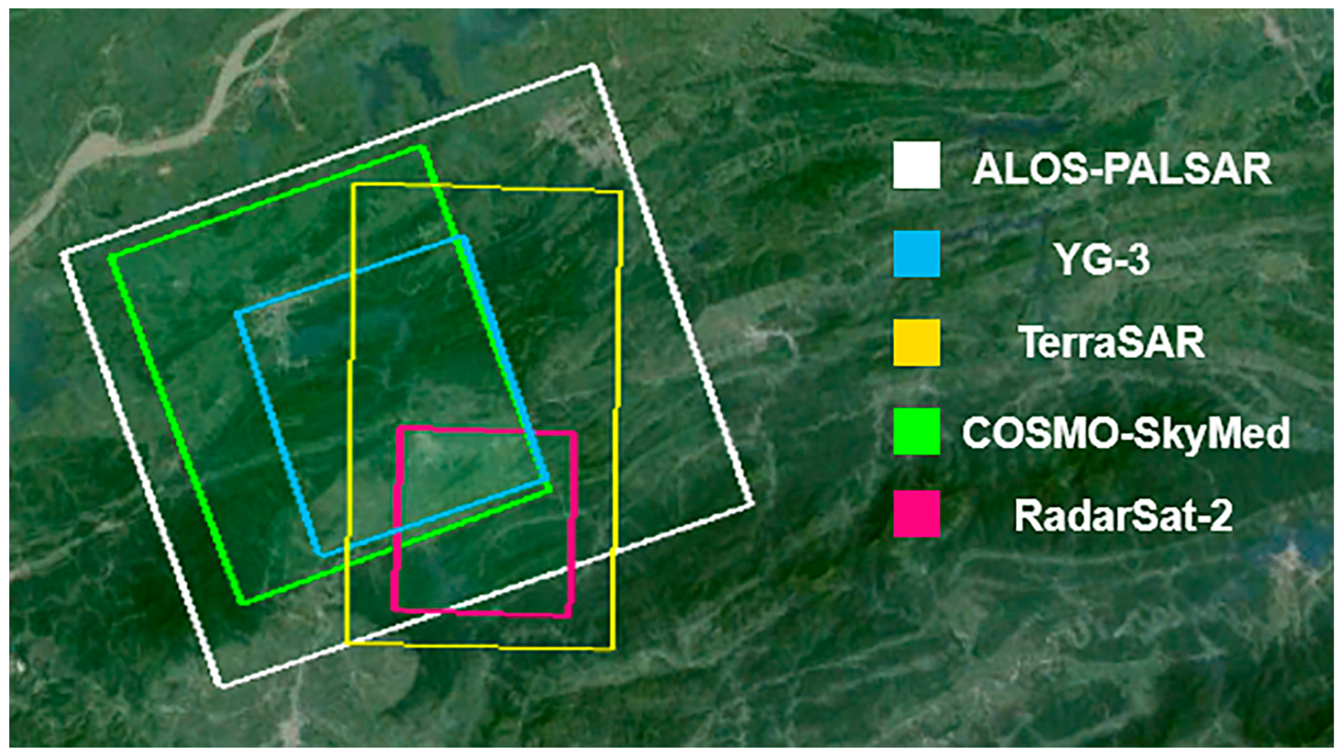
  • The geometric performance of five representative high-resolution SAR satellites: ALOS, TerraSAR-X, Cosmo-SkyMed, RadarSat-2, and Chinese YG-3, is evaluated on the same benchmark with the rational function model (RFM) based on the Xianning validation field. The experimental analysis concerns the geolocation accuracies of the above satellite products and provides a reference for the application in the field of spaceborne SAR.
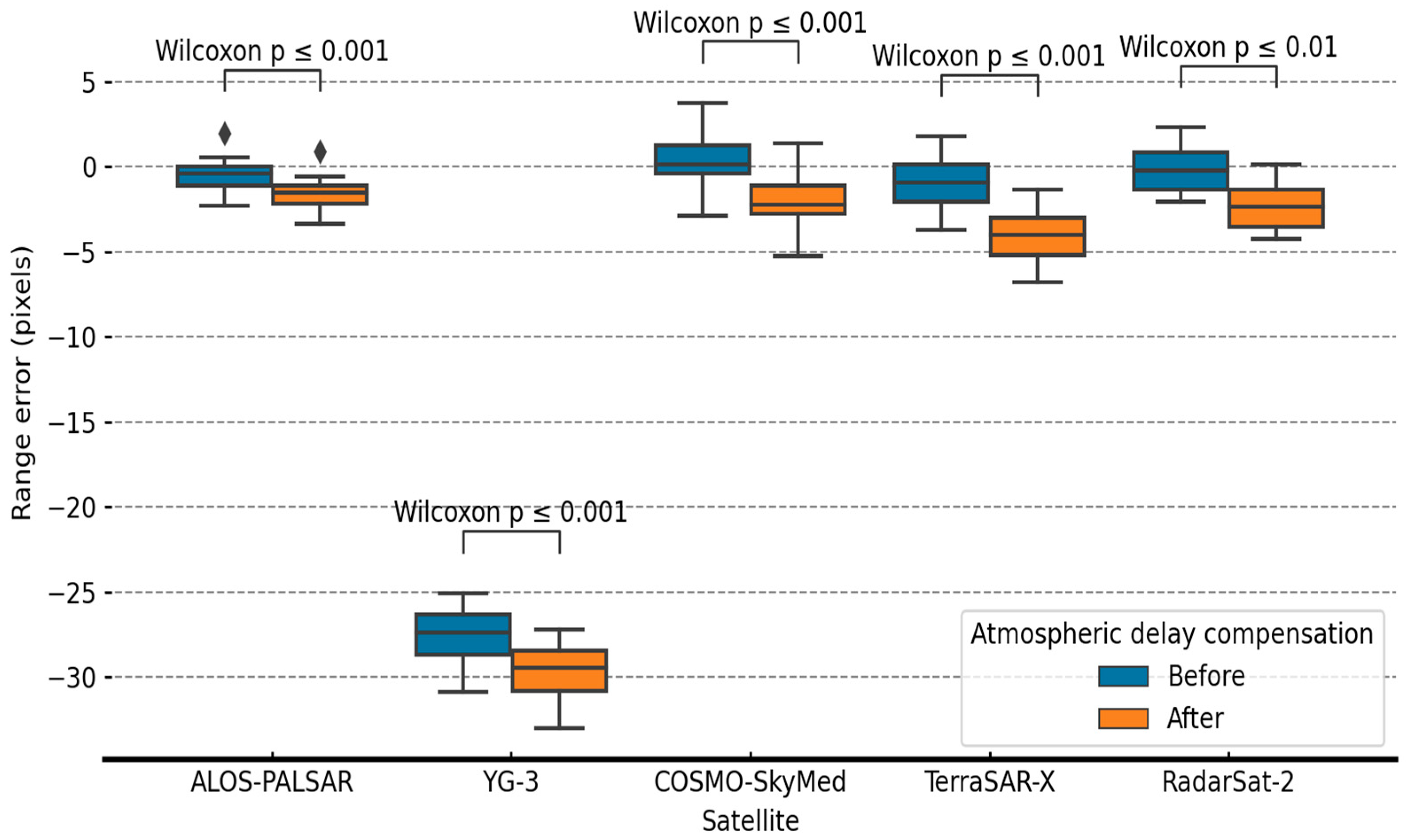
  • An atmospheric delay correction model is used to evaluate the APD, and the experimental results show that a rough atmospheric correction result might have been added to the parameters of each satellite product in advance.
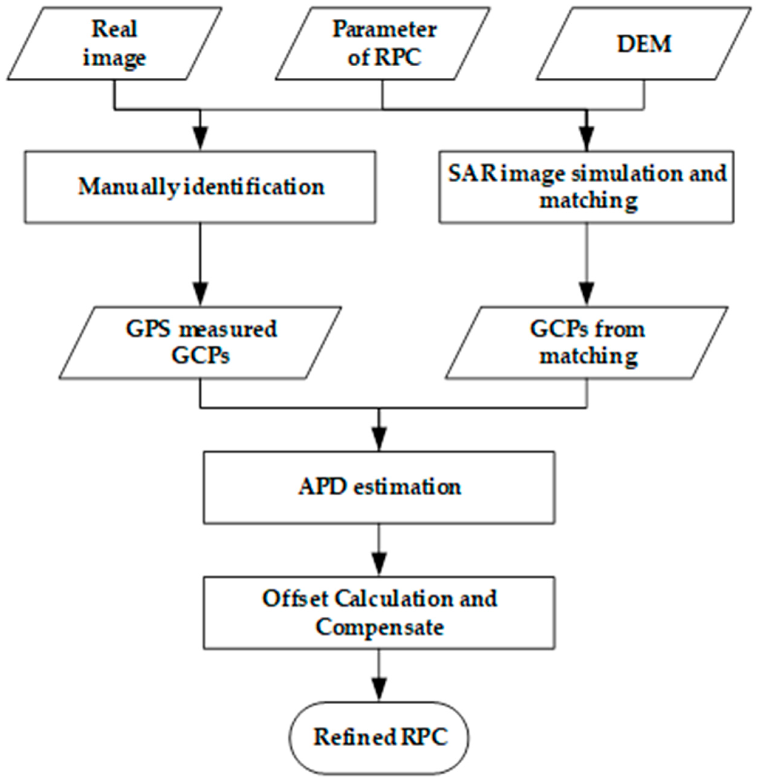
  • A simulated images-based method is proposed to obtain ground control points (GCPs) for SAR images. It is proven effective by the experiment results, which provides an option for improving the geolocation accuracy on rough terrain areas.
This paper focuses on the geolocation evaluation of multiple spaceborne SAR images. Section 2 describes the proposed geolocation evaluation method and Section 3 shows the dataset, test-field area, experimental results, and discussion. Finally, Section 4 presents the conclusions.

2. Methods

The accuracy verification process in this paper is presented in Figure 1. Firstly, image coordinates of GCPs obtained through GPS measurement were manually identified for each image. To minimize errors arising from manual identification, DEM data were utilized as a reference, and a simulated image was generated based on the RPC parameters of the real image. The matched GCPs were then automatically extracted through a matching process. Finally, the affine transformation parameters were computed based on the two types of GCPs after APD correction, and the image’s geolocation accuracy was subsequently verified.

2.1. Rational Function Model for SAR Images

In the field of spaceborne SAR application, accurately assessing the geolocation accuracy of SAR images is a critical task. One commonly used geometric model for geolocation is the range-Doppler (R-D) model. However, using the R-D model for comparative analysis of geolocation accuracy across different SAR images can be challenging because of the need to develop different processing modules based on the auxiliary data. The rational function model (RFM), which is calculated and fitted from the R-D model, can be a better choice for the comparative analysis of different satellites’ SAR images.
The RFM has been widely accepted as a substitute for the rigorous geometric model in SAR image processing [20]. Its application has gained significant interest among scholars in related fields, and its ability to substitute the rigorous R-D model has been thoroughly investigated [21,22,23,24,25,26,27]. The RFM describes the correspondence between the coordinates  x n ,   y n  on the image and the geographical coordinates  X n , Y n , Z n  in a simple form and can avoid the unstable calculation of the rigorous model due to too many unknown parameters.
Let  r n ,   c n    and  B n , Y n , Z n  be the normalized coordinates of  x n ,   y n    and  X n , Y n , Z n  by the scale and offset parameters provided in the rational polynomial coefficient (RPC) file. The RFM has the following form [21]:
r n = p 1 B n , L n , H n p 2 B n , L n , H n c n = p 3 B n , L n , H n p 4 B n , L n , H n
where  r n ,   c n  are calculated coordinates of the point on the nth image in sample and line directions. The  p i i = 1 , 2 , 3 , 4  are third-order polynomials of  B n , L n , H n ; for example, the form of the polynomial  p 1  is as follows:
p 1 = h 0 + h 1 H + h 2 L + h 3 B + h 4 H L + h 5 H B + h 6 L B + h 7 H 2 + h 8 L 2 + h 9 B 2 + h 10 H L B + h 11 H 2 L + h 12 H 2 B + h 13 L 2 H + h 14 L 2 B + h 15 H B 2 + h 16 L B 2 + h 17 H 3 + h i 18 L 3 + h 19 B 3
where  h i i = 0 , 1 , , 19  are the rational polynomial coefficients of  p 1 . All coefficients of  p i i = 1 , 2 , 3 , 4  can be found in the RPC file.
In this paper, the affine transformation model was used in bias compensation for the RFM [24]. This model establishes the relationship between the coordinates  x , y  on the image and the geographical coordinates  X , Y , Z , which has the following form [18]:
Δ x = x x = x + a 0 + a 1 x + a 2 y Δ y = y y = y + b 0 + b 1 x + b 2 y
where  Δ x    and  Δ y  are errors between the measured point coordinates  x , y  on the image and the calculated coordinates  x , y  corresponding to GCP coordinates  X , Y , Z  by using RFM. Parameters of affine transformation  a 0 , a 1 , a 2 , b 0 , b 1 , b 2  can be solved using a few GCPs. It is noteworthy that the each parameter in the affine transformation model can be used to compensate for the specific errors with physical significance [28].
The spaceborne SAR systems measure ground targets by pulse ranging and coherent focusing in side-view geometry. Its accuracy mainly depends on accurate orbital measurement and precise time counting in both range and azimuth directions, and distinct form optical satellites are simultaneously influenced by imaging attitude. The orbital records, range measurement, and instrumental stability account for primary error resources [29]. Error  Δ x  in the sample direction results from a ranging error  Δ R , mainly due to inaccurate ranging trip timing. A timing offset is caused mainly by APD, cross-track positional error, and an offset parameter,  a 0 , can compensate for instrumental drift. The remaining scale timing error in the sample direction resulting from the cross-track position error and the sample rate estimation error can be absorbed by  a 1 .
Doppler shift due to an along-track position and velocity measurement error, and spacecraft clock shift, are caused an offset,  Δ y , in the line direction, and thus can be compensated by parameter  b 0 . The remaining azimuth scale errors due to inaccurate estimation of pulse repetition frequency (PRF) can be compensated by parameter  b 1 . Moreover, parameters  a 2  and  b 2  in a small amount can also compensate for the scale errors in line and sample directions.

2.2. Estimation of Atmospheric Propagation Delay

When a radar pulse passes through the atmosphere, the refractive index of the air changes along the ray path. As a result, the speed of the signal in the atmosphere is slower than in the vacuum, resulting in an atmospheric propagation delay,  Δ L , which can be calculated by:
Δ L = Δ Z · M F θ
Considering an incident angle  θ , actual propagation delay,  Δ L , can be expressed in the form of the product of zenith delay,  Δ Z , and a projection function,  M F θ . A simple projection function can be written as [13]:
M F θ = 1 cos θ
For radar signals with frequencies greater than 30 GHz, the zenith atmospheric propagation delay can be decomposed into two main parts: the non-dispersive part, i.e., the tropospheric propagation delay, and the dispersive part, i.e., the ionospheric propagation delay.
The effect of ionospheric zenith delay,  Δ Z i o n , which is inversely proportional to the square of the signal frequency, can be calculated by the total number of electrons (TEC) as follows:
Δ Z i o n = 40.28 · T E C f 2
where  f  is the frequency of the radar pulse and TEC is expressed in 1016 units (called total election content units, TECU), with typical TECUs ranging from 5 to 10.
The actual TEC values can be obtained from the Global Ionospheric Map (GIM) provided daily by the European Center for Orbit Determination (CODE) or the German Aerospace Center (DLR) [30]. The ionospheric propagation delay has the greatest impact on the L-band and the least on the X-band of the SAR system.
The troposphere-caused signal delays are not related to the radar frequency. According to [7], a calculation model integrating the influence of dry air, water vapor, liquid water, and for tropospheric zenith delay,  Δ Z t r o , and atmospheric refractivity,  N , was given as:
Δ Z t r o = 10 6 z 0 z a t o m N d z N = k 1 · P d T d r y   a i r + k 2 · e T + k 3 · e T 2 w e t   a i r + k 4 · W c l o u d l i q u i d   w a t e r
where  z  is the propagation path from Earth’s surface,  z 0 , to the upper limit of the atmosphere,  z a t o m P d  and  e  are the atmospheric pressure (mbar) of dry and wet air, T is the temperature (K), and  W c l o u d  is the cloud water content (g/m3). The constants are  k 1 = 77.6   K / mbar k 2 = 6.0   K / mbar k 3 = 3.75 × 10 5   K 2 / mbar , and  k 4 = 1.45   m 3 / g . In (7), the first term is the propagation delay related to dry air, and the second and third terms provide the effects related to water vapor. The effects of water droplets by the fourth term can be ignored concerning the total propagation delay [31].

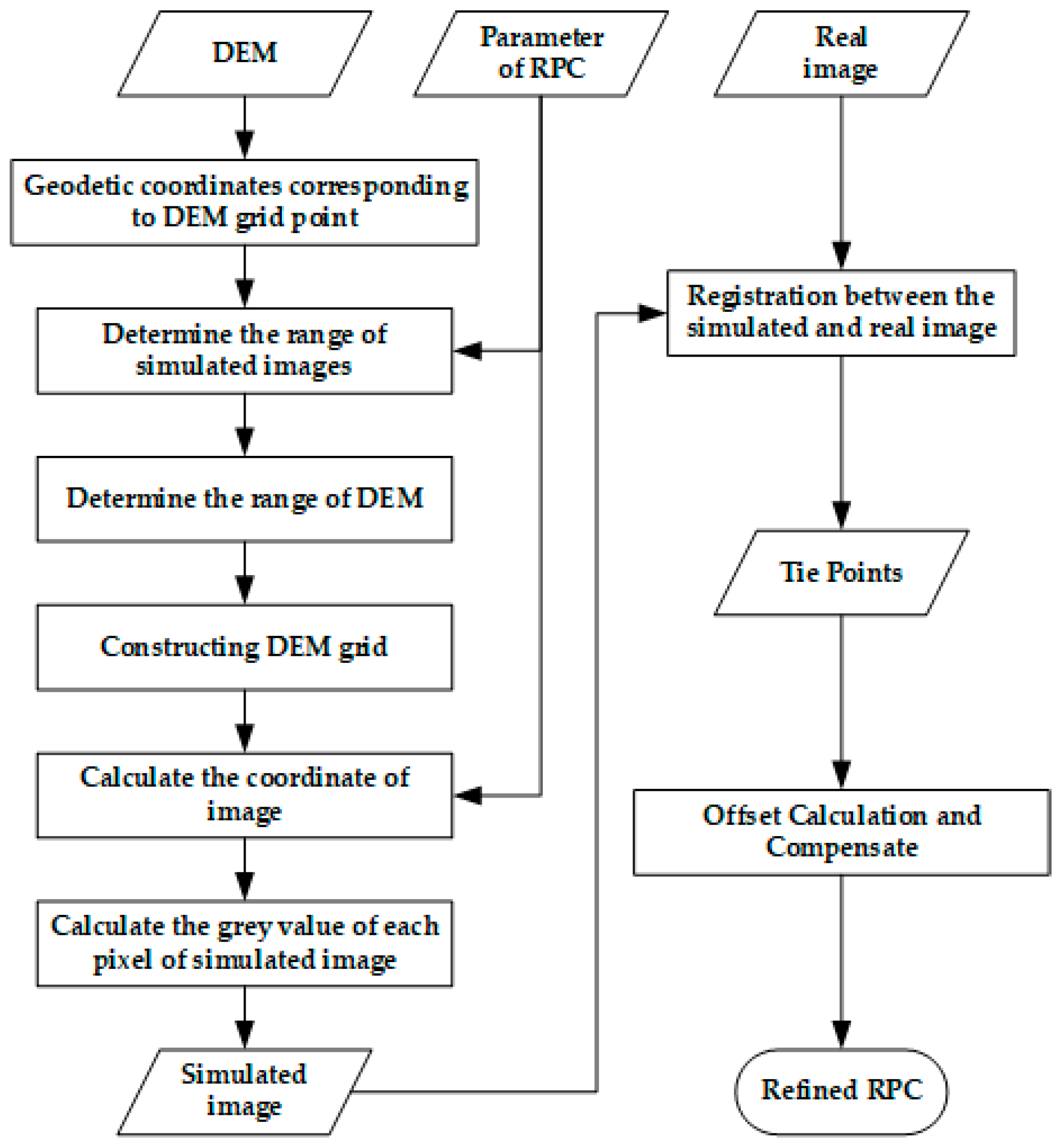
2.3. DEM-Based SAR Image Simulation

Manual point selection on images may introduce some errors during point identification, which is especially significant in high-resolution images. According to [32,33], such errors are usually around one pixel, which needs to be considered. In areas with large terrain fluctuations, such as mountains and hills, the GCPs are hard to identify due to geometric distortions such as overlapping, shadow, and foreshortening. Therefore, obtaining GCP from reference data such as DOM and DEM through image-matching technology is undoubtedly labor-saving and effective.
The SAR image simulation technology can generate an image similar to a real image in geometric and radiometric properties [34,35,36,37]. Since the accuracy of various parameters used for simulation and reference data is known, reliable GCPs can be obtained by real-to-simulated image matching. In areas with flat terrain, the simulation of SAR images usually needs to know the detailed parameters of the SAR system, as well as the types of ground objects and electronic characteristics. However, such information is not required in mountainous areas because the image grey value is mainly influenced by geometric distortions, including layover, shadow, and foreshortening [37]. Zhang G. et al. proposed an incoherent approach to generating SAR-simulated images using RFM [38]. As shown in Figure 2, this method involves three steps, outlined below.
  • Determine the range of the simulated image and the used DEM. Firstly, extract the covering areas of the DEM and convert them to geodetic coordinates under the WGS84 coordinate system via a transformation based on the RFM. Then, determine the range of the simulated image by combining the covering area of the DEM and real image.
  • DEM interpolation and simulated image coordinate solution: Since the resolutions of the DEM and the real SAR image are inconsistent, a DEM with the same resolution as the real image is generated via bilinear interpolation. Then, the SAR image coordinates corresponding to each point on the DEM are solved by using the RFM, building the pixel-corresponding relation between the DEM and the simulated SAR image.
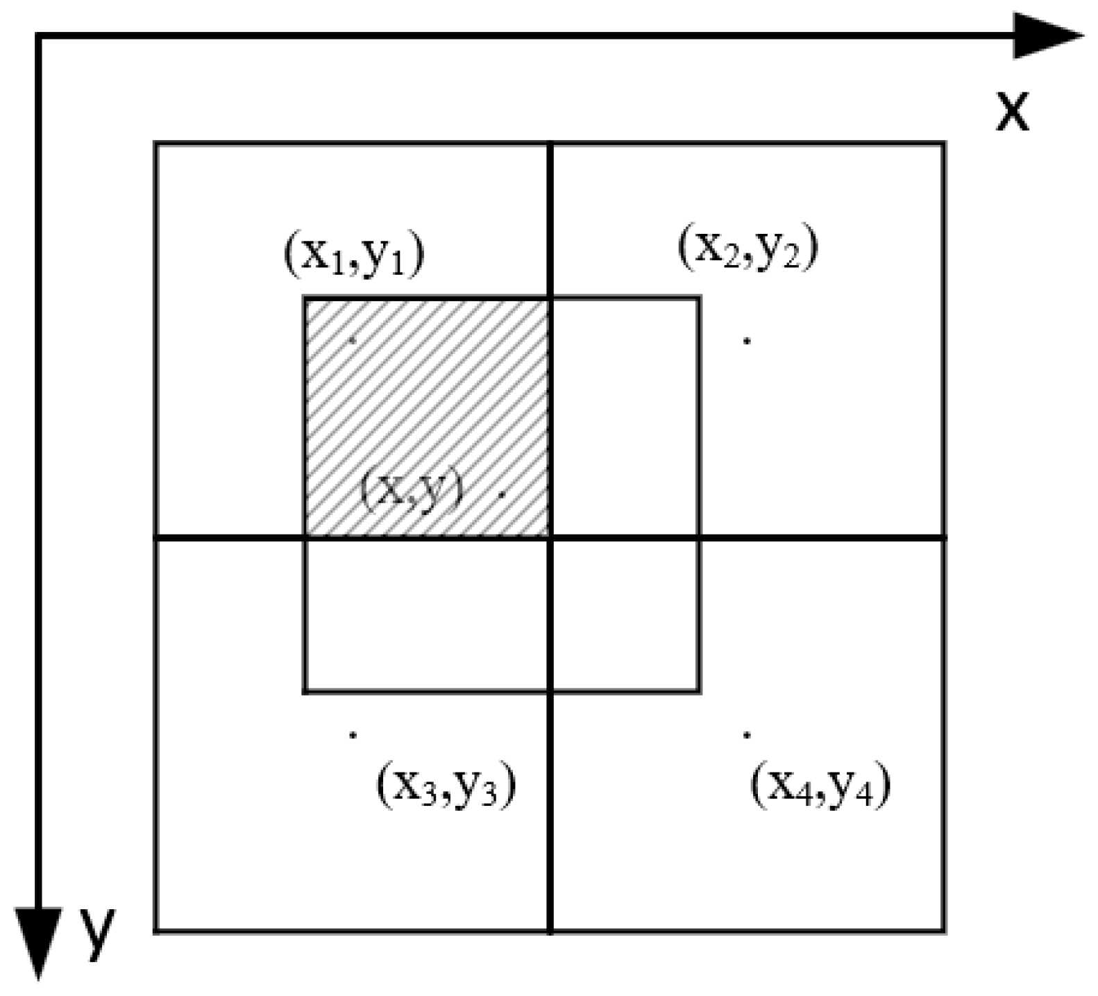
  • Determine the backscattered power (grey value) of the simulated image. For one cell (X, Y, Z) in DEM, the coordinate of the corresponding pixel (x, y) in the simulated image can be calculated by using the RFM, and  x i ,   y i , i = 1 , 2 , 3 , 4  are grid points surrounding (x, y) (as shown in Figure 3). For each pixel in DEM, its contribution of grey value to four adjacent pixels is based on the size of the intersection area. As highlighted in Figure 3, the contribution of (x, y) to pixel  x 1 ,   y 1  is  1 x + x 1 · 1 y + y 1 . Due to the imaging characteristics of SAR and the geometric distortions such as layover, perspective shrinkage, and shadow, the actual relationship may not be a one-to-one correspondence. Some pixels may have higher brightness when one pixel in the simulated image consists of multiple ground units [39].
Once the correspondence between the simulated image and DEM is calculated, the correspondence between the real and simulated images can be further established by image registration. Finally, the geolocation error of the real image can be solved with the known 3D coordinates of the DEM.

3. Experiment and Result Analysis

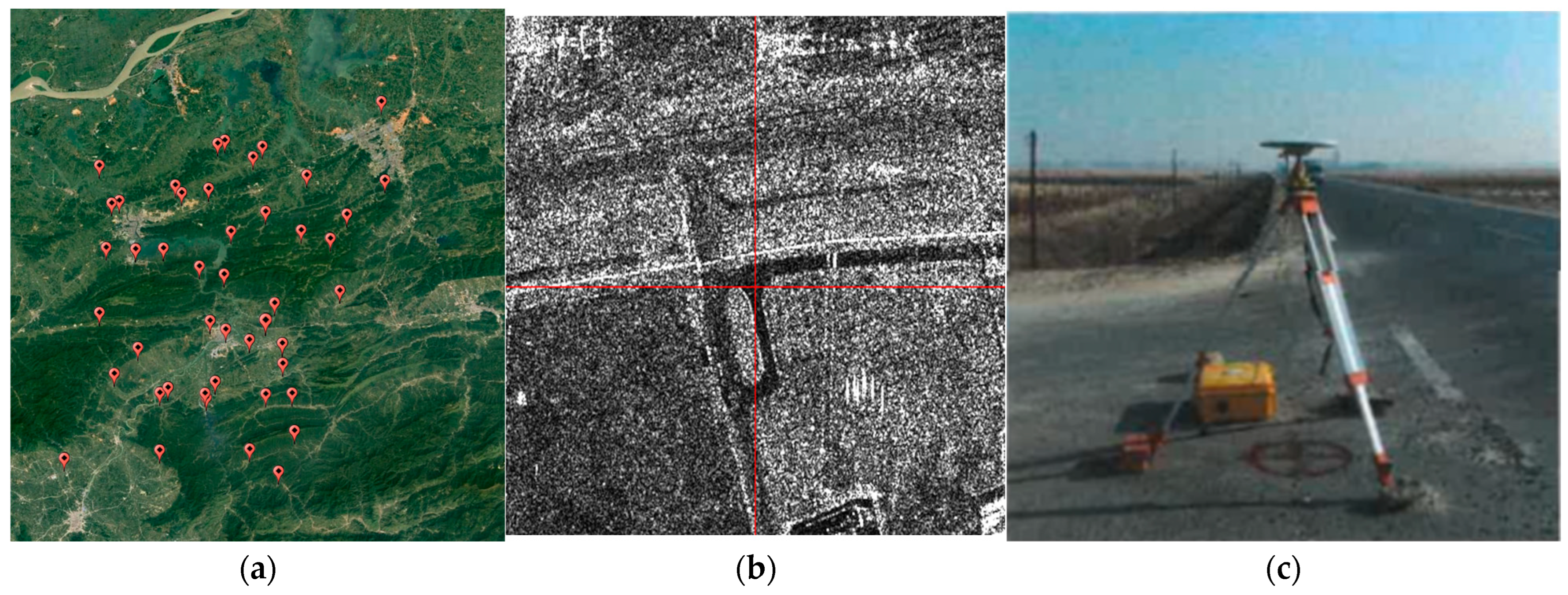
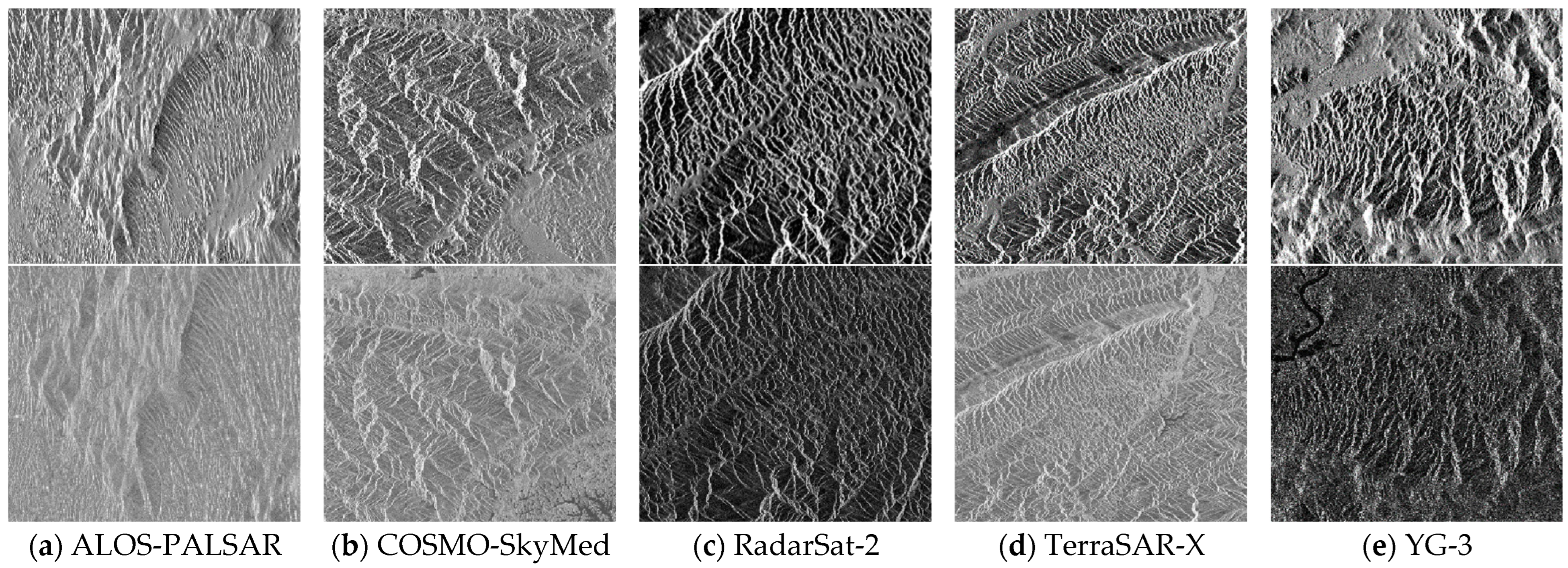
3.1. Dataset and Test-Field Area

The validation field is located in the Xianning area, south of Hubei province, central China (N29°, E113°). The area has different surface features (urban, residential, arable land, and rivers) and its total extent is about 400 km2, with elevation ranging from 0 m to 1500 m. In our previous work, the optical high-resolution satellite images were validated in the same test field [40].
The experiment collected five high-resolution SAR images within the Xianning validation field range, and each image’s coverage area is shown in Figure 4. The detailed information of the SAR images used is summarized in Table 1.
To evaluate the geometric accuracy of SAR images, the use of GCPs is essential. Two kinds of GCPs were used for validation: GCPs obtained by manual measurement with the GPS filed survey, and GCPs obtained by matching from the SAR simulated image.
For GPS surveyed GCPs, a total of 45 points were collected in this area (as shown in Figure 5), evenly distributing on each image, and the accuracy of these GCPs is about 10 cm in ground space. Manual identification of GCPs always brings some errors, especially on SAR images. As far as possible to reduce such errors, the principle of selecting GCPs is to select the intersection point or inflection point of the road or other strongly reflective objects [16].
Due to the imaging geometric characteristics of SAR images, obtaining reliable GCPs by GPS field measurement is difficult, while the area covered by SAR images is rough terrain. Suppose DEM data are available in this area. In that case, it is conceivable to obtain GCPs by auto-matching between the simulated and real images since they are geometrically consistent, and the simulated image has a relatively high geolocation accuracy [38]. To generate simulated images, the DEM used was 10 m-spaced, generated by ZiYuan-3 (ZY-3) stereo images. This DEM has a planimetric accuracy of 3 m and an elevation accuracy of 2 m. The details of the simulated and real images are shown in Figure 6.
In this paper, two kinds of GCPs were used in validation: those obtained by manual measurement with the GPS field survey and those by auto-matching between the simulated image and the real image. In the experiment, the known GCPs were divided into two groups: one group was used as GCPs in the geometric model, and the other as check points (CPs) to validate the model itself. The GCP-laid scheme is as shown in Figure 7.
The RMSE criterion assesses the geolocation accuracy of the SAR image. Considering the N CPs true ground coordinate { l a t i t u d e ,   l o n g i t u d e ,   h e i g h t i ,   i N }, the projected points’ coordinates {   x , y i ,   i N } on the image can be obtained via RFM. The true image points’ coordinates {   x , y i ,   i N  } were manually measured or matched from a simulated image. The RMSE was calculated according to the following formula:
R M S E x = 1 N i = 1 N x i x i 2 R M S E y = 1 N i = 1 N y i y i 2 R M S E p l a n e = 1 N i = 1 N x i x i 2 + y i y i 2

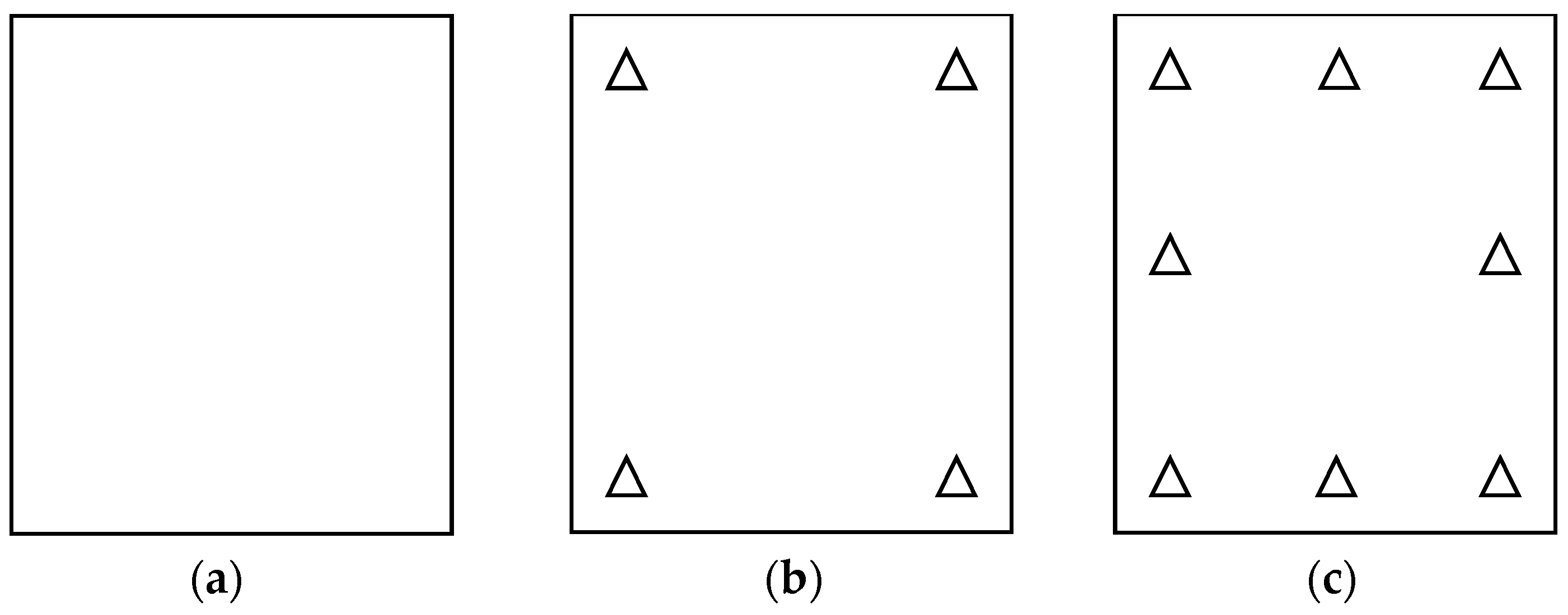
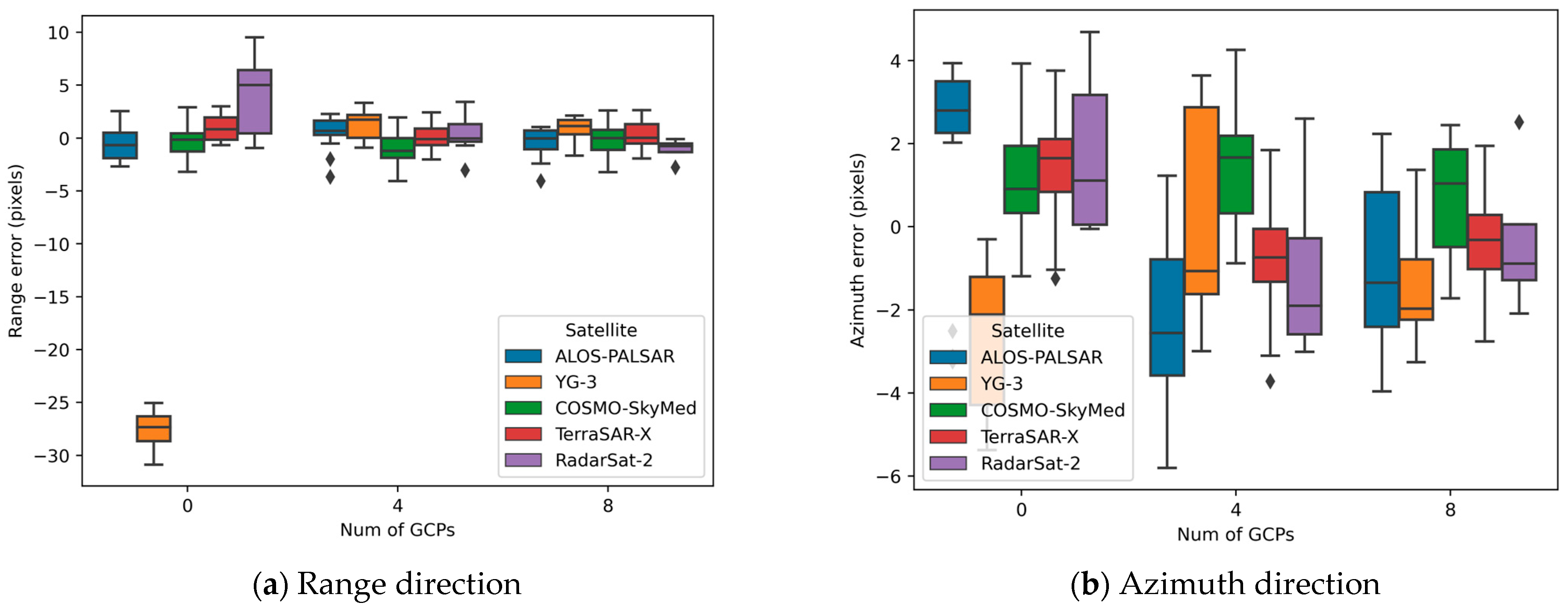
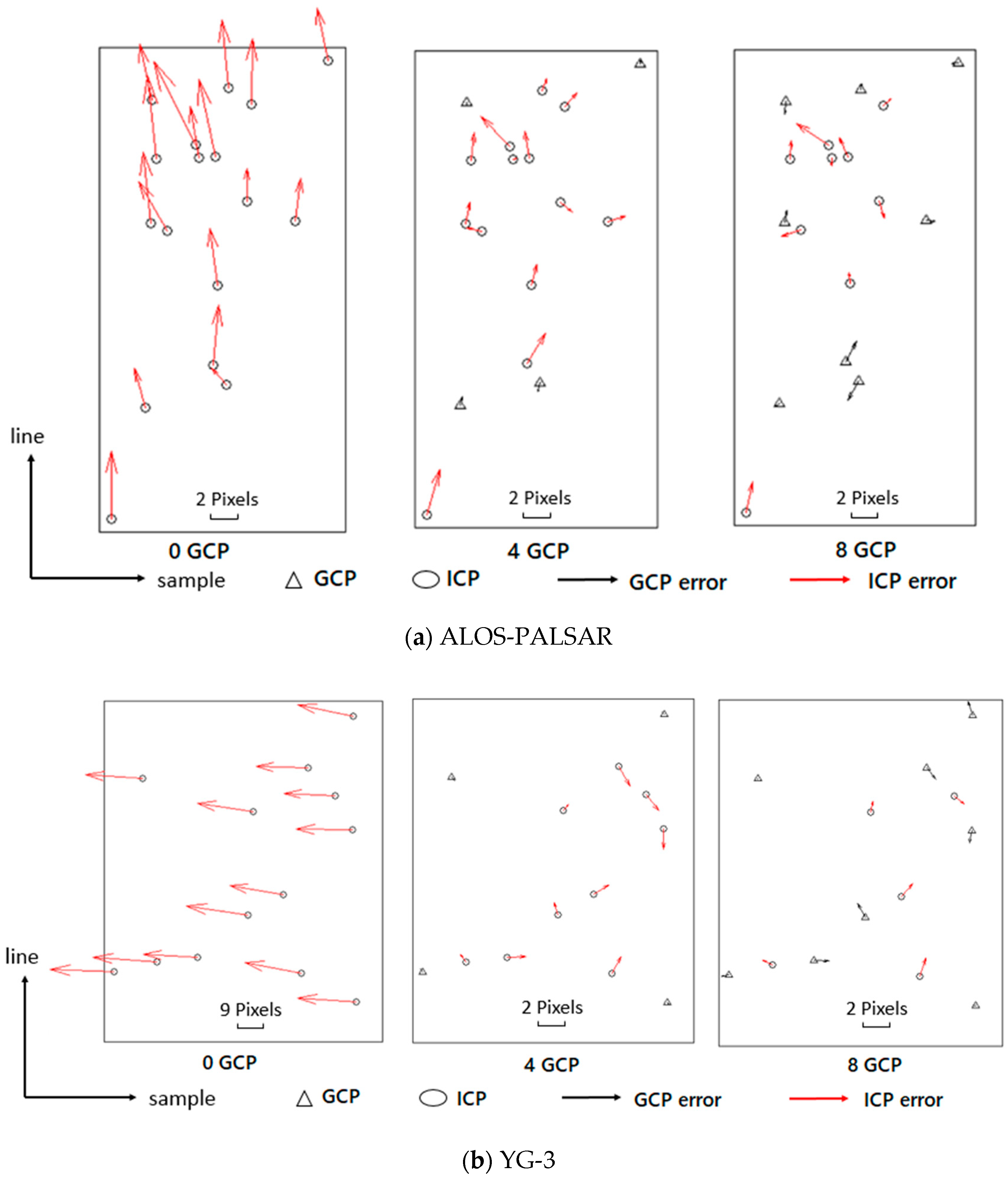
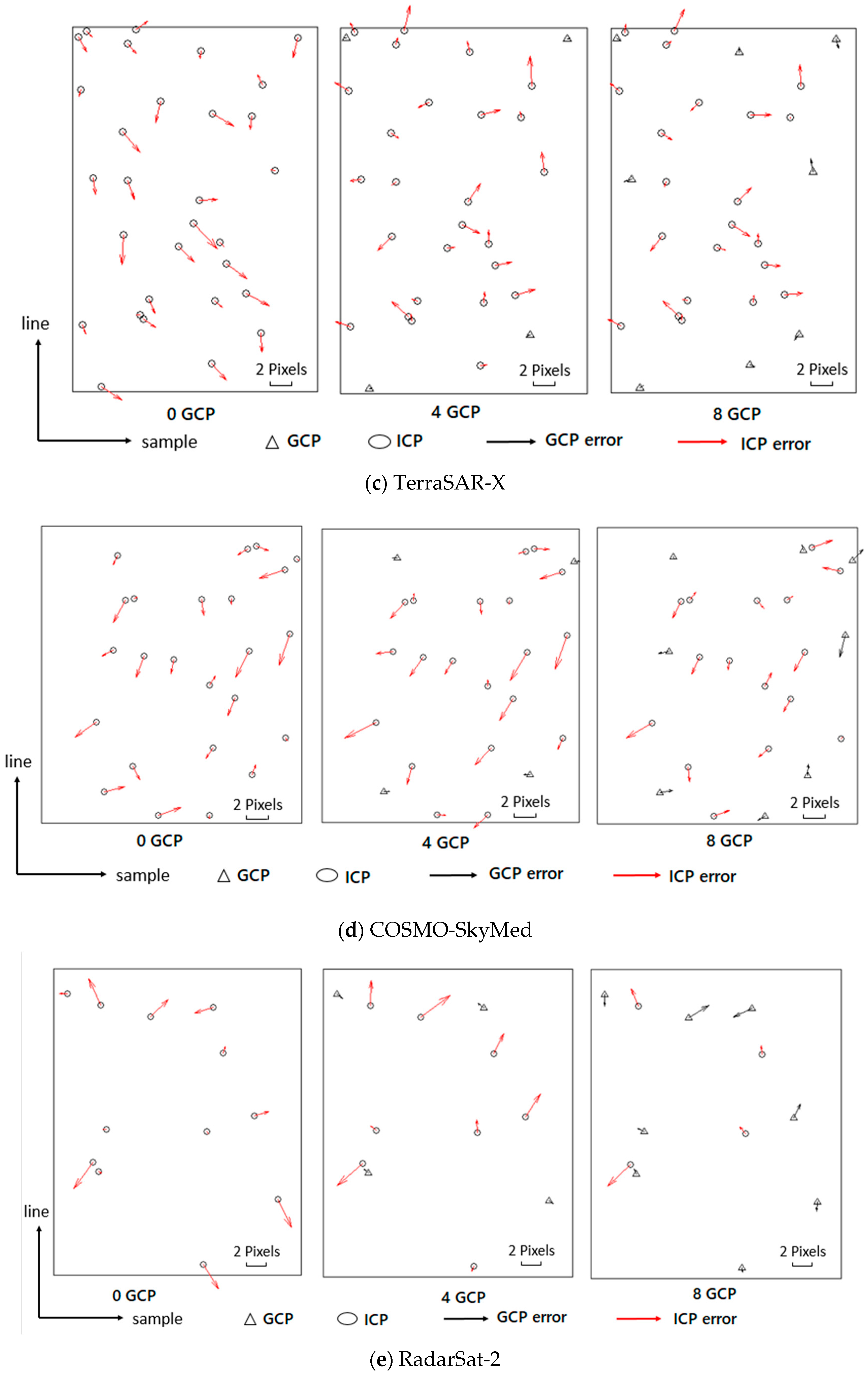
3.2. Accuracy Assessment with GPS Measured GCPs

The atmospheric propagation delay includes ionospheric and tropospheric delay. The ionospheric delay was estimated based on CODE’s global TEC data [30]. Moreover, the meteorological data used to estimate tropospheric delay were the 3D numerical weather model data from the Regional Reference Frame Sub-Commission for Europe (EUREF) analysis centers [41]. The ionospheric and tropospheric slant delay of the five satellite images was calculated and compensated, and the results are shown in Table 2.
The ionospheric delay had a minor influence on X-band satellites, while it ranged in the centimeter level for C-band and the meter level for L-band. Since the local time when satellite imaging occurred was during the daytime, the ionosphere had a higher TEC, which caused a higher delay for each satellite. The tropospheric slant delays of YG-3, COSMO-SkyMed, TerraSAR-X, and RadarSat-2 images were on the same magnitude of about 2.7 m since the troposphere delays do not depend on radar frequency. Due to a larger incident angle, the tropospheric slant delay of the ALOS-PALSAR image was higher, which was 3.2 m. The total atmospheric slant delays of five satellite images were calculated and compensated by considering the ionospheric and tropospheric delays, and the results before and after APD correction are presented in Figure 8.
As shown in Figure 8, after both ionospheric and tropospheric delays were compensated, the slant range accuracy was worse than the accuracy without propagation delay compensation. The decrease in slant range accuracy suggests that a rough APD correction was incorporated during product generation. A Wilcoxon signed-rank test [42] was performed to compare the results before and after APD correction. The test revealed a significant correlation between the two groups (p < 0.05), which suggests that there is a statistically significant relationship between the two sets of data.
As mentioned in [43], using a static model, an ionospheric delay of 2.6 cm and a coarse tropospheric delay have been calculated and annotated in TerraSAR-X products. This result indicates that a coarse APD correction could be incorporated into the single-look slant range images, which agrees with the conclusions of previous works [13,16,18,19,44].
After considering the APD, the geolocation accuracy of each image was analyzed and verified using the affine transform model based on different schemes of laid GCPs, as follows in Table 3.
According to the results in Figure 9 and Figure 10b, the YG-3 image orientation result without GCPs showed consistent residual distributions of check points mainly in the range direction. As seen in Table 3, the range geolocation RMSE of YG-3 reached 27.645 pixels and was worse than the results of the other four satellites. This range offset may be caused by a sum contribution of the platform velocity error and electronic hardware delay. Figure 10a indicates that the ALOS-PALSAR image has an azimuth RMSE, amounting to 3.278 pixels according to Table 3, which may result from the drift in the spacecraft clock or the along-track platform velocity error. COSMO-SkyMed, TerraSAR-X, and RadarSat-2 had approximately the same RMSE on the order of 1.5 pixels in the range direction, and their azimuth RMSE were 1.708, 1.826, and 1.936 pixels, respectively. Figure 10c–e failed to reveal any obvious systematic errors, which might be caused by the manual measurement procedure of point identification. Despite the errors introduced in the manual measurement procedure and atmosphere propagation, the performance of COSMO-SkyMed, TerraSAR-X, and RadarSat-2 was still outstanding among the five SAR satellites.
With four GCPs laid in the corners, the results of YG-3 and ALOS-PALSAR were significantly improved to the 2-pixel level, as shown in Figure 9 and Figure 10, while the errors of COSMO-SkyMed, TerraSAR-X, and RadarSat-2 slightly changed. When more GCPs were added, the RMSE of all images remained larger than 1.2 pixels.
The above results show that the errors introduced during manual identification of the GPS measured GCPs cannot be ignored. Therefore, when applying high-precision SAR images, it is necessary to consider adding other methods of reference data to eliminate systematic errors.

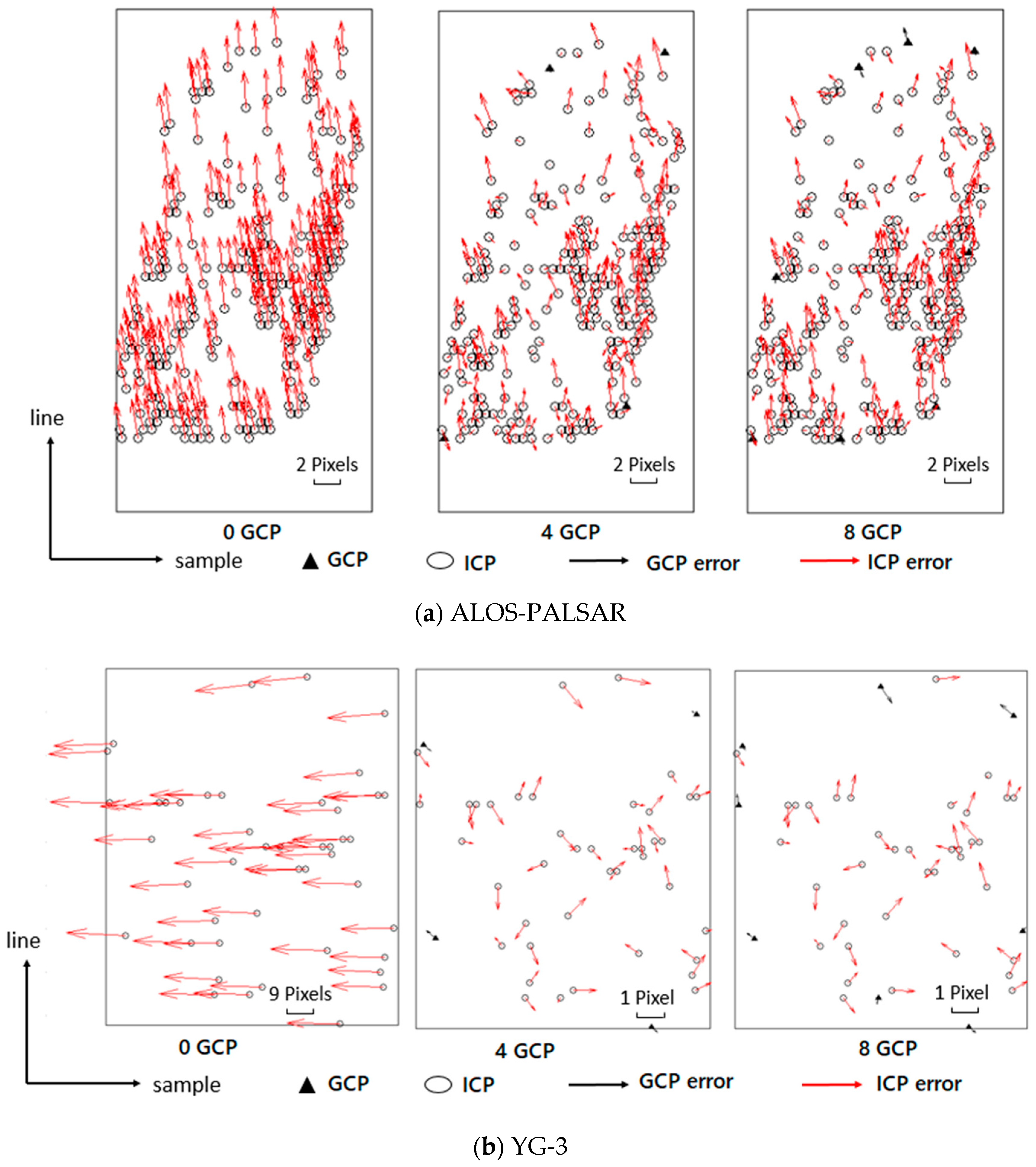
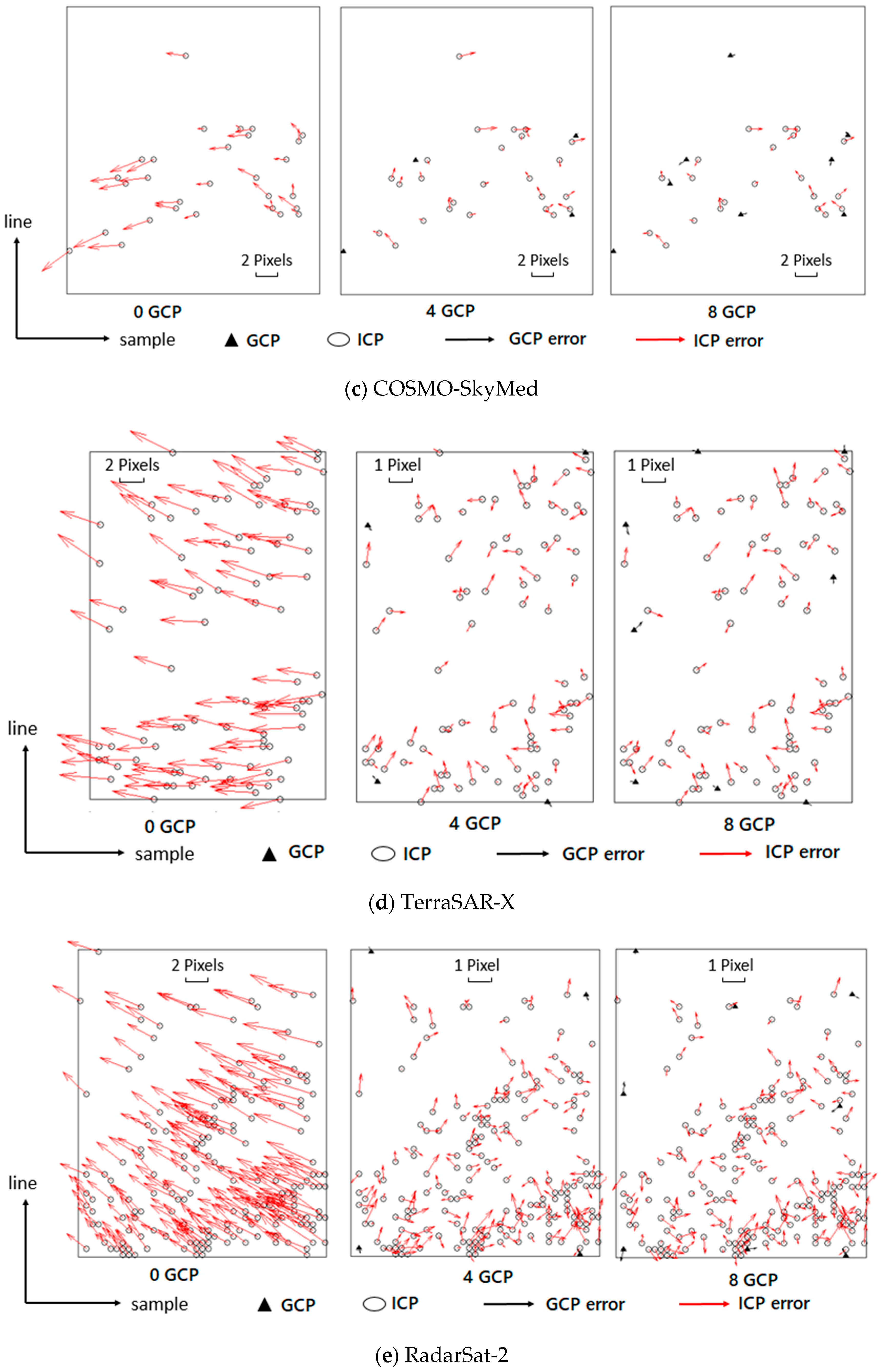
3.3. Accuracy Assessment with Simulated GCPs from Simulated Image

As discussed in Section 3.2, the errors introduced by manual identification of GPS measured GCPs are difficult to eliminate by laying 4 GCPs in the corners. In this section, the GCPs obtained by matching the simulated image and the real image could alleviate errors in manual point selection, and the validation results are shown. The CPs used for verifying were obtained in the same way as GCPs, and the affine transform model was used to fit the GCPs.
According to Table 4 and residual distributions in Figure 11a,b, the systematic errors of ALOS-PALSAR and YG-3 were almost identical to the previous results in size and direction, which indirectly proves that the points obtained by simulated image matching are effective.
However, Table 4 shows that the range of RMSEs of RadarSat-2, COSMO-SkyMed, and TerraSAR-X amounted to 2.644, 5.63, and 5.648 pixels, more significant than the 1.448, 1.506, and 1.493 pixels in Table 3 and Figure 9. Moreover, Figure 11 indicates obvious systematic errors in the range dimension. To determine the newly introduced errors, several main factors need to be considered in the procedure of SAR image simulation: the DEM used, the satellite view geometry, and the APD.
In Section 3.2, we have analyzed and compensated for the effects of APD. Moreover, the proposed simulation method employs RFM as a replacement for the rigorous R-D model to generate simulated images that are geometrically consistent with real images, which means the view geometry was the same. Considering that the accuracy of the geolocation of the simulated image is dependent on the accuracy of the DEM used in the simulation, hence, the remaining source of error can be attributed to the quality of the DEM used. In this study, we used the DEM product of the ZY-3 satellite, which provides an elevation accuracy of 2 m. According to [24], the relationship between slant error,  δ R , and elevation error,  δ h , could be described as:
δ h = δ R · cos θ
where  θ  is the incidence angle. Taking the incidence angle of 30°, for example, an error of 2 m in elevation can provide a slant error of 2.309 m. For a simulated image with a sample spacing of 5 m, the error generated is no more than one pixel. In other words, for ALOS, the errors introduced by the DEM used in the simulation procedure were less than 1 pixel, and for COSMO-SkyMed and YG-3, the errors were around 1 pixel.
Fortunately, unlike the manually measured GCP, the error caused by the DEM in the simulation can be eliminated by multiple GCPs. With four GCPs laid in the corners, the results of almost all images can achieve accuracy better than 1 pixel in both range and azimuth direction. Therefore, the GCPs obtained by simulation and matching can effectively improve the positioning accuracy of SAR images, especially in places with large terrain fluctuations such as hills and mountains. Acquisition of GCP by GPS measurement or CRs in these places is usually labor-intensive and difficult. In this case, using the method proposed in this article to obtain GCPs becomes an alternative.

4. Conclusions

This study evaluated the orientation accuracy of five satellite images using RFM based on the Xianning test field. The results show that, as a representative of Chinese spaceborne SAR satellites, there is still a considerable gap between the YG-3 and foreign spaceborne SAR satellites. In comparison, the performance of COSMO-SkyMed, TerraSAR-X, and RadarSat-2 was better than YG-3 and ALOS-PALSAR, amounting to an RMSE of a 2-pixel level without GCPs. The atmospheric delay correction results showed that after APD compensation, the accuracy in the slant range direction was lower than the previous results without delay correction. The decrease in slant range accuracy indicated that a rough APD correction was incorporated into the single-look slant range images during product generation.
Moreover, a simulated image-based method was proposed to obtain GCPs by matching points between the simulated and real images. The obtained GCPs can be used to reduce the errors imported by artificial point identification. According to the results, the geolocation accuracy of almost all images can be improved to better than an RMSE of 1 pixel in both range and azimuth dimensions. The simulated image-based method provides an alternative way to evaluate and improve geolocation accuracy on rough terrain areas.

Author Contributions

Conceptualization, G.Z. and T.W.; methodology, B.J. and M.D.; software, B.J.; validation, B.J., X.L. and Q.C.; formal analysis, B.J.; investigation, B.J.; resources, F.W.; data curation, M.D. and S.L.; writing—original draft preparation, B.J.; writing—review and editing, B.J. and T.W.; visualization, X.L.; supervision, X.D.; project administration, F.W.; funding acquisition, G.Z. All authors have read and agreed to the published version of the manuscript.

Funding

This research was funded by the Foundation Strengthening Fund Project, grant number 2021-JCJQ-JJ-0251.

Data Availability Statement

Not applicable.

Acknowledgments

The authors would like to thank the reviewers and editors for their helpful comments.

Conflicts of Interest

The authors declare no conflict of interest.

References

  1. Tang, L.; Tang, W.; Qu, X.; Han, Y.; Wang, W.; Zhao, B. A Scale-Aware Pyramid Network for Multi-Scale Object Detection in SAR Images. Remote Sens. 2022, 14, 973. [Google Scholar] [CrossRef]
  2. Zhao, B.; Han, Y.; Wang, H.; Tang, L.; Liu, X.; Wang, T. Robust Shadow Tracking for Video SAR. IEEE Geosci. Remote Sens. Lett. 2021, 18, 821–825. [Google Scholar] [CrossRef]
  3. Yoon, Y.T.; Eineder, M.; Yague-Martinez, N.; Montenbruck, O. TerraSAR-X Precise Trajectory Estimation and Quality Assessment. IEEE Trans. Geosci. Remote Sens. 2009, 47, 1859–1868. [Google Scholar] [CrossRef]
  4. Schubert, A.; Jehle, M.; Small, D.; Meier, E. Influence of Atmospheric Path Delay on the Absolute Geolocation Accuracy of TerraSAR-X High-Resolution Products. IEEE Trans. Geosci. Remote Sens. 2010, 48, 751–758. [Google Scholar] [CrossRef]
  5. Balss, U.; Eineder, M.; Fritz, T.; Breit, H.; Minet, C. Techniques for high accuracy relative and absolute localization of TerraSAR-X/TanDEM-X data. In Proceedings of the 2011 IEEE International Geoscience and Remote Sensing Symposium, IEEE, Vancouver, BC, Canada, 24–29 July 2011; pp. 2464–2467. [Google Scholar] [CrossRef] [Green Version]
  6. Eineder, M.; Minet, C.; Steigenberger, P.; Cong, X.; Fritz, T. Imaging Geodesy—Toward Centimeter-Level Ranging Accuracy with TerraSAR-X. IEEE Trans. Geosci. Remote Sens. 2011, 49, 661–671. [Google Scholar] [CrossRef]
  7. Cong, X.; Balss, U.; Eineder, M.; Fritz, T. Imaging Geodesy—Centimeter-Level Ranging Accuracy with TerraSAR-X: An Update. IEEE Geosci. Remote Sens. Lett. 2012, 9, 948–952. [Google Scholar] [CrossRef]
  8. Shimada, M. Ortho-Rectification and Slope Correction of SAR Data Using DEM and Its Accuracy Evaluation. IEEE J. Sel. Top. Appl. Earth Obs. Remote Sens. 2010, 3, 657–671. [Google Scholar] [CrossRef]
  9. Luscombe, A. Image quality and calibration of RADARSAT-2. In Proceedings of the 2009 IEEE International Geoscience and Remote Sensing Symposium, Cape Town, South Africa, 12–17 July 2009; Volume 2, pp. 757–760. [Google Scholar] [CrossRef]
  10. Williams, D.; LeDantec, P.; Chabot, M.; Hillman, A.; James, K.; Caves, R.; Thompson, A.; Vigneron, C.; Wu, Y. RADARSAT-2 Image Quality and Calibration Update. In Proceedings of the EUSAR 2014; 10th European Conference on Synthetic Aperture Radar, Berlin, Germany, 3–5 June 2014; pp. 1–4. [Google Scholar]
  11. Schubert, A.; Miranda, N.; Geudtner, D.; Small, D. Sentinel-1A/B Combined Product Geolocation Accuracy. Remote Sens. 2017, 9, 607. [Google Scholar] [CrossRef] [Green Version]
  12. Deng, M.; Zhang, G.; Zhao, R.; Li, S.; Li, J. Improvement of Gaofen-3 Absolute Positioning Accuracy Based on Cross-Calibration. Sensors 2017, 17, 2903. [Google Scholar] [CrossRef] [Green Version]
  13. Wang, W.; Liu, J.; Qiu, X. Decimeter-Level Geolocation Accuracy Updated by a Parametric Tropospheric Model with GF-3. Sensors 2018, 18, 2197. [Google Scholar] [CrossRef] [Green Version]
  14. Deng, M.; Zhang, G.; Cai, C.; Xu, K.; Zhao, R.; Guo, F.; Suo, J. Improvement and Assessment of the Absolute Positioning Accuracy of Chinese High-Resolution SAR Satellites. Remote Sens. 2019, 11, 1465. [Google Scholar] [CrossRef]
  15. Deng, M.; Zhang, G.; Zhao, R.; Zhang, Q.; Li, D.; Li, J. Assessment of the geolocation accuracy of YG-13A high-resolution SAR data. Remote Sens. Lett. 2018, 9, 101–110. [Google Scholar] [CrossRef]
  16. Zhang, G.; Zhao, R.; Li, S.; Deng, M.; Guo, F.; Xu, K.; Wang, T.; Jia, P.; Hao, X. Stability Analysis of Geometric Positioning Accuracy of YG-13 Satellite. IEEE Trans. Geosci. Remote Sens. 2022, 60, 1–12. [Google Scholar] [CrossRef]
  17. Yunjun, Z.; Fattahi, H.; Pi, X.; Rosen, P.; Simons, M.; Agram, P.; Aoki, Y. Range Geolocation Accuracy of C-/L-Band SAR and its Implications for Operational Stack Coregistration. IEEE Trans. Geosci. Remote Sens. 2022, 60, 1–19. [Google Scholar] [CrossRef]
  18. Schubert, A.; Small, D.; Jehle, M.; Meier, E. COSMO-skymed, TerraSAR-X, and RADARSAT-2 geolocation accuracy after compensation for earth-system effects. In Proceedings of the 2012 IEEE International Geoscience and Remote Sensing Symposium, IEEE, Munich, Germany, 22–27 July 2012; pp. 3301–3304. [Google Scholar] [CrossRef] [Green Version]
  19. Nitti, D.O.; Nutricato, R.; Lorusso, R.; Lombardi, N.; Bovenga, F.; Bruno, M.F.; Chiaradia, M.T.; Milillo, G. On the geolocation accuracy of COSMO-SkyMed products. In Proceedings of the SAR Image Analysis, Modeling, and Techniques XV, SPIE, Toulouse, France, 21–24 September 2015; Volume 9642, pp. 69–80. [Google Scholar] [CrossRef]
  20. Dowman, I.; Tao, V. An update on the use of rational functions for photogrammetric restitution. ISPRS Highlights 2002, 7, 22–29. [Google Scholar]
  21. Zhang, G.; Zhu, X. A study of the RPC model of TerraSAR-X and COSMO-SkyMed SAR imagery. Int. Arch. Photogramm. Remote Sens. Spat. Inf. Sci. 2008, 37, 321–324. [Google Scholar]
  22. Zhang, G.; Fei, W.; Li, Z.; Zhu, X.; Li, D. Evaluation of the RPC Model for Spaceborne SAR Imagery. Photogramm. Eng. Remote Sens. 2010, 76, 727–733. [Google Scholar] [CrossRef]
  23. He, X.; Wei, X.; Zhang, L.; Balz, T.; Liao, M. RPC modeling for spaceborne SAR and its aplication in radargrammetry. In Proceedings of the 2010 IEEE International Geoscience and Remote Sensing Symposium, Honolulu, HI, USA, 25–30 July 2010; pp. 3600–3603. [Google Scholar] [CrossRef]
  24. Zhang, L.; Balz, T.; Liao, M. Satellite SAR geocoding with refined RPC model. ISPRS J. Photogramm. Remote Sens. 2012, 69, 37–49. [Google Scholar] [CrossRef]
  25. Jiang, W.; Yu, A.; Dong, Z.; Wang, Q. Comparison and Analysis of Geometric Correction Models of Spaceborne SAR. Sensors 2016, 16, 973. [Google Scholar] [CrossRef]
  26. Bagheri, H.; Schmitt, M.; d’Angelo, P.; Zhu, X.X. A framework for SAR-optical stereogrammetry over urban areas. ISPRS J. Photogramm. Remote Sens. 2018, 146, 389–408. [Google Scholar] [CrossRef]
  27. Akiki, R.; Marí, R.; De Franchis, C.; Morel, J.-M.; Facciolo, G. Robust rational polynomial camera modelling for SAR and pushbroom imaging. In Proceedings of the 2021 IEEE International Geoscience and Remote Sensing Symposium IGARSS, Brussels, Belgium, 11–16 July 2021; pp. 7908–7911. [Google Scholar] [CrossRef]
  28. Zhang, G.; Li, Z.; Pan, H.; Qiang, Q.; Zhai, L. Orientation of Spaceborne SAR Stereo Pairs Employing the RPC Adjustment Model. IEEE Trans. Geosci. Remote Sens. 2011, 49, 2782–2792. [Google Scholar] [CrossRef]
  29. Curlander, J.C.; McDonough, R.N. Synthetic Aperture Radar; Wiley: Hoboken, NJ, USA, 1991; Volume 11. [Google Scholar]
  30. Zhao, R.; Zhang, G.; Deng, M.; Yang, F.; Chen, Z.; Zheng, Y. Multimode Hybrid Geometric Calibration of Spaceborne SAR Considering Atmospheric Propagation Delay. Remote Sens. 2017, 9, 464. [Google Scholar] [CrossRef] [Green Version]
  31. Hanssen, R.F. Radar Interferometry Data Interpretation and Error Analysis. In Radar Interferometry Data Interpretation and Error Analysis; Springer Science & Business: Berlin, Germany, 2001. [Google Scholar]
  32. Raggam, H.; Perko, R.; Gutjahr, K.; Kiefl, N. Accuracy Assessment of 3D Point Retrieval from TerraSAR-X Data Sets. In Proceedings of the European Conference on Synthetic Aperture Radar, Eurogress Aachen, Germany, 7–10 June 2010. [Google Scholar]
  33. Zhao, R.; Jiang, Y.; Zhang, G.; Deng, M.; Yang, F. Geometric Accuracy Evaluation of YG-18 Satellite Imagery Based on RFM. Photogramm. Rec. 2017, 32, 33–47. [Google Scholar] [CrossRef]
  34. Franceschetti, G.; Migliaccio, M.; Riccio, D. The SAR simulation: An overview. In Proceedings of the International Geoscience & Remote Sensing Symposium, Firenze, Italy, 10–14 July 1995. [Google Scholar]
  35. Guindon, B.; Adair, M. Analytic Formulation of Spaceborne SAR Image Geocoding and “Value-Added” Product Generation Procedures using Digital Elevation Data. Can. J. Remote Sens. 1992, 18, 2–12. [Google Scholar] [CrossRef]
  36. Kimura, H.; Kodaira, N. Simulation and comparison of JERS-1 and ERS-1 SAR images. In Proceedings of the International Geoscience & Remote Sensing Symposium, Tokyo, Japan, 18–21 August 1993. [Google Scholar]
  37. Gelautz, M.; Frick, H.; Raggam, J.; Burgstaller, J.; Leberl, F. SAR image simulation and analysis of alpine terrain. ISPRS J. Photogramm. Remote Sens. 1998, 53, 17–38. [Google Scholar] [CrossRef]
  38. Zhang, G.; Qiang, Q.; Luo, Y.; Zhu, Y.; Gu, H.; Zhu, X. Application of RPC Model in Orthorectification of Spaceborne SAR Imagery: Application of RPC model in orthorecitification of spaceborne SAR imagery. Photogramm. Rec. 2012, 27, 94–110. [Google Scholar] [CrossRef]
  39. Wang, H.; Cheng, Q.; Wang, T.; Zhang, G.; Wang, Y.; Li, X.; Jiang, B. Layover Compensation Method for Regional Spaceborne SAR Imagery Without GCPs. IEEE Trans. Geosci. Remote Sens. 2021, 59, 8367–8381. [Google Scholar] [CrossRef]
  40. Zheng, X.; Huang, Q.; Wang, J.; Wang, T.; Zhang, G. Geometric Accuracy Evaluation of High-Resolution Satellite Images Based on Xianning Test Field. Sensors 2018, 18, 2121. [Google Scholar] [CrossRef] [Green Version]
  41. Bruyninx, C. The EUREF Permanent Network: A multi-disciplinary network serving surveyors as well as scientists. GeoInformatics 2004, 7, 32–35. [Google Scholar]
  42. Woolson, R.F. Wilcoxon Signed-rank Test. Wiley Encycl. Clin. Trials 2007, 1–3. [Google Scholar]
  43. Eineder, M.; Schattler, B.; Breit, H.; Fritz, T.; Roth, A. TerraSAR-X SAR products and processing algorithms. In Proceedings of the 2005 IEEE International Geoscience and Remote Sensing Symposium, 2005, IGARSS ’05, Seoul, Republic of Korea, 25–29 July 2005; Volume 7, pp. 4870–4873. [Google Scholar] [CrossRef]
  44. Small, D.; Zuberbühler, L.; Schubert, A.; Meier, E. Terrain-flattened gamma nought Radarsat-2 backscatter. Can. J. Remote Sens. 2011, 37, 493–499. [Google Scholar] [CrossRef] [Green Version]
Figure 1. Flow chart of SAR image geolocation evaluation.
Remotesensing 15 01794 g001
Figure 2. Flow chart of SAR image simulation and RPC compensation.
Remotesensing 15 01794 g002
Figure 3. Grey value calculation in simulated image.
Remotesensing 15 01794 g003
Figure 4. Thumbnail of multiple images’ coverage.
Remotesensing 15 01794 g004
Figure 5. (a) Distribution of GPS GCPs in the Xianning test field. (b) One GCP in the SAR image. (c) Measurement photograph of surveyors in the field.
Remotesensing 15 01794 g005
Figure 6. Details of simulated and real images. For each satellite, the top is the simulated image and the bottom is the real image.
Remotesensing 15 01794 g006
Figure 7. GCP-laid scheme: (a) no GCP, (b) four GCPs in corners, and (c) eight GCPs.
Remotesensing 15 01794 g007
Figure 8. Geolocation accuracy before and after atmospheric delay compensation. (solid diamonds ◆ represent outliers).
Remotesensing 15 01794 g008
Figure 9. Geolocation accuracy with different numbers of GCPs. (solid diamonds ◆ represent outliers).
Remotesensing 15 01794 g009
Figure 10. Distributions of check point errors based on field measurement GCPs.
Remotesensing 15 01794 g010aRemotesensing 15 01794 g010b
Figure 11. Distributions of check point errors with GCPs obtained from the simulated image.
Remotesensing 15 01794 g011aRemotesensing 15 01794 g011b
Table 1. Details of SAR imagery in the Xianning validation field.
SatelliteALOSCOSMO-SkyMedRadarSat-2TerraSAR-XYG-3
CountryJapanItalyCanadaGermanyChina
Orbit height692 km620 km800 km515 km600 km
Imaging time22 December 200822 July 201218 March 201324 July 201227 April 2012
Range spacing5.0 m3.0 m1.6 m1.2 m3.0 m
Azimuth spacing3.0 m2.5 m2.8 m3.3 m3.0 m
Width of image50 km × 70 km40 km × 40 km20 km × 20 km30 km × 50 km30 km × 30 km
Incident angle34°32°31°30°30°
Orbit direction and LookDescending, rightDescending, rightDescending, rightDescending, rightDescending, right
Imaging modeFine ResolutionHimageUltraFineStripMapStrip
Data levelLevel 1.1SCSSLCSSCL1B
Polarization modesHHHHHHHHHH
Image size9344 × 18,43219,604 × 22,3348794 × 10,86118,700 × 27,69413,469 × 16,426
Table 2. Ionospheric, tropospheric delay, and accuracy after compensation of SAR images.
SatelliteMean Ionospheric Slant Delay (m)Mean Tropospheric Slant Delay (m)Slant Range RMSE of CPs after Compensation (Pixels)
ALOS-PALSAR1.78543.21941.923
YG-30.05692.698829.765
COSMO-SkyMed0.05582.78482.540
TerraSAR-X0.03692.67854.323
RadarSat-20.12562.70712.665
Table 3. Geolocation accuracy of SAR images with GCPs by GPS field measurement.
SatelliteNumber of GCPsNumber of CPsRMSE of GCPs (Pixels)RMSE of CPs (Pixels)
RangeAzimuthPlaneRangeAzimuthPlane
ALOS-PALSAR017——————1.8703.2783.773
4130.2110.8580.8841.6932.9163.372
890.8461.5061.7281.7022.2192.796
YG-3013——————27.6453.12927.822
490.4110.4860.6371.9052.4253.084
851.3011.6272.0831.5242.0982.593
COSMO-SkyMed024——————1.4481.7082.240
4200.6990.0040.6991.7281.9422.599
8120.9771.2571.5921.4671.4422.057
TerraSAR-X030——————1.5061.8262.367
4260.3270.0560.3321.3241.4771.984
8220.5480.8050.9741.3711.2631.864
RadarSat-2012——————1.4931.9362.445
480.6010.4600.7571.8012.1762.824
841.1891.0821.4891.4891.7522.300
Table 4. Geolocation accuracy of SAR images with GCPs by simulated image matching.
SatelliteNumber of GCPsNumber of CPsRMSE of GCP (Pixels)RMSE of CP (Pixels)
RangeAzimuthPlaneRangeAzimuthPlane
ALOS-PALSAR0238——————1.1048.0658.140
42340.0800.1780.1960.3411.0381.092
82300.1800.4690.5020.3391.0931.197
YG-3045——————28.8851.25328.912
4410.4270.3450.5490.7410.8491.127
8370.4520.5540.7150.7010.9091.148
COSMO-SkyMed029——————2.6441.1202.872
4250.2210.2490.3331.0910.7911.348
8210.4830.4550.6640.9320.8191.240
TerraSAR-X084——————5.6301.6355.863
4800.3250.4300.5380.8360.9371.255
8760.4200.5110.6610.7830.8761.175
RadarSat-20183——————5.6483.3176.550
41790.1750.4090.4450.7780.8671.165
81750.4450.5980.7450.7040.8121.075
Disclaimer/Publisher’s Note: The statements, opinions and data contained in all publications are solely those of the individual author(s) and contributor(s) and not of MDPI and/or the editor(s). MDPI and/or the editor(s) disclaim responsibility for any injury to people or property resulting from any ideas, methods, instructions or products referred to in the content.

