Communication

Skillful Seasonal Prediction of Typhoon Track Density Using Deep Learning

1
College of Meteorology and Oceanography, National University of Defense Technology, Changsha 410000, China
2
College of Advanced Interdisciplinary Studies, National University of Defense Technology, Nanjing 210000, China
3
National Centre for Atmospheric Science and Department of Meteorology, University of Reading, Reading RG6 6AH, UK
4
State Key Laboratory of Severe Weather, Chinese Academy of Meteorological Sciences, Beijing 100000, China
5
Ministry of Education Key Laboratory for Earth System Modeling, Department of Earth System Science, Tsinghua University, Beijing 100000, China
6
PLA Troop 32033, Haikou 570100, China
*
Author to whom correspondence should be addressed.
These authors contributed equally to this work.
Remote Sens. 2023, 15(7), 1797; https://doi.org/10.3390/rs15071797
Submission received: 24 February 2023 / Revised: 22 March 2023 / Accepted: 25 March 2023 / Published: 28 March 2023
(This article belongs to the Topic Big Data and Artificial Intelligence)

Abstract

:
Tropical cyclones (TCs) seriously threaten the safety of human life and property especially when approaching a coast or making landfall. Robust, long-lead predictions are valuable for managing policy responses. However, despite decades of efforts, seasonal prediction of TCs remains a challenge. Here, we introduce a deep-learning prediction model to make skillful seasonal prediction of TC track density in the Western North Pacific (WNP) during the typhoon season, with a lead time of up to four months. To overcome the limited availability of observational data, we use TC tracks from CMIP5 and CMIP6 climate models as the training data, followed by a transfer-learning method to train a fully convolutional neural network named SeaUnet. Through the deep-learning process (i.e., heat map analysis), SeaUnet identifies physically based precursors. We show that SeaUnet has a good performance for typhoon distribution, outperforming state-of-the-art dynamic systems. The success of SeaUnet indicates its potential for operational use.

Graphical Abstract

1. Introduction

A tropical cyclone (TC) is a weather system mostly formed over a tropical ocean. The associated strong winds and torrential rain pose a serious threat to the lives and property safety of people under its influence. The Western North Pacific (WNP) is the most active region for TCs, accounting for about 30% of the global TCs [1]. The long-term TC activity in the WNP is affected by both atmospheric and oceanic factors [2], with significant variation from seasonal to decadal timescales [3,4,5,6]. These factors include sea-surface temperature (SST) anomalies in the Pacific Ocean, in particular the El Niño–Southern Oscillation (ENSO) [7,8], SST anomalies in the Indian Ocean [9], SST anomalies in the Atlantic Ocean [10], subtropical high [6], Pacific decadal oscillation (PDO) [11], and interdecadal Pacific oscillation (IPO) [12], among others.
TC activity on the seasonal timescale is mainly controlled by slowly evolving SST conditions and large-scale atmospheric circulation, which provide potential sources for TC seasonal prediction [2,13]. The techniques in TC seasonal prediction mainly include statistical models [14,15,16], dynamic models [17,18,19,20], and hybrid statistical–dynamic models [21,22]. Although dynamic models are better than statistical models in physical interpretability, statistical models are still a mainstream choice today because of the initial condition errors and uncertainty of physical-process representation in dynamic models [23]. Hybrid statistical–dynamic models, which integrate the advantages of both dynamic and statistical models, can have better prediction skills [15]. The existing approaches have focused on the interannual variation of TC frequency (TCF) and accumulated cyclone energy (ACE) at basin wide or regional scales [14,17,19,24]. There are no prediction techniques tailored for the spatial distribution of TCs, due to the limited understanding and prediction of the complicated dynamic processes for local TC activity [18,20].
Seasonal climate prediction is considered nonlinear behavior [25] and due to the shortcomings of the aforementioned methods in solving nonlinear problems, the annual TC spatial distribution has not been predicted effectively previously. Deep learning, a new data-driven technology, shows unprecedented capability in understanding and reconstructing geophysical fields [26,27]. Using the explosive amount of General Circulation Model (GCM) outputs, deep learning technology can significantly improve both weather and climate predictions, such as the ENSO [28,29], Asian summer monsoon [30], and Arctic sea ice [31] predictions. Lower computational cost compared with traditional dynamic models is an advantage of deep learning. In this study, we introduce a new framework of SeaUnet, which is a fully convolutional neural network architecture, to predict the seasonal spatial track density of typhoons.

2. Data and Methods

Our SeaUnet model uses monthly maps of 500-hPa geopotential height (H500), which is linked with TC moving [32], subsurface ocean temperature (average temperature of 300-m sea water below the sea surface, SubSST), which provides energy for the development of TC [33], and zonal vertical shear (difference between 200- and 800-hPa zonal winds, ushear), which is related to the large-scale atmospheric circulation [34], in three consecutive months before the start time (e.g., three consecutive months of March–April–May before the start time of June) to identify predictors. The predictand is the TC track density over WNP in the typhoon season of June to November. We also test the performance of SeaUnet for the total number of typhoons in the WNP.

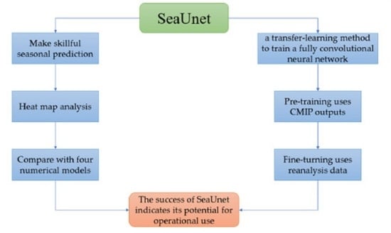
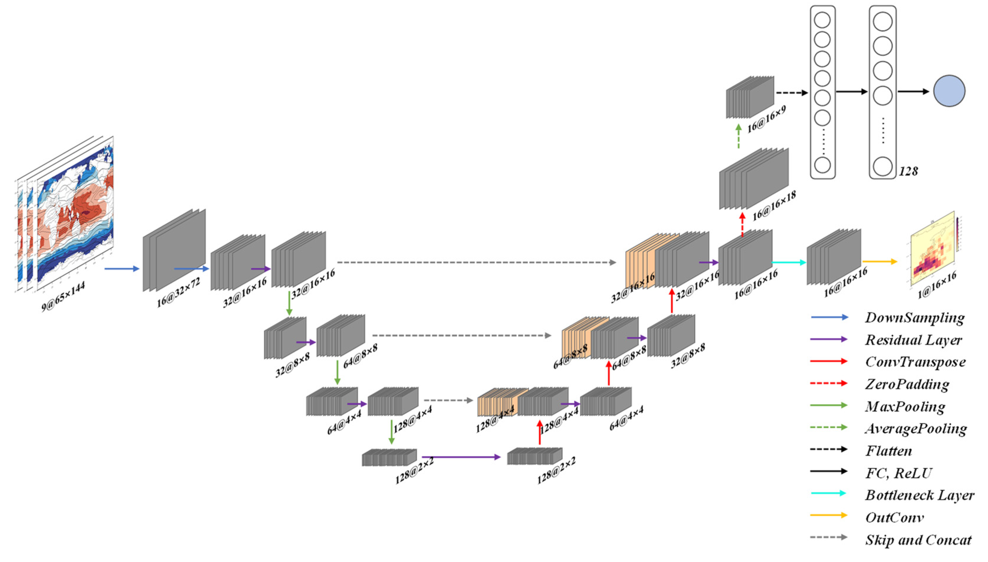
2.1. Architecture of the SeaUnet Model

The architecture of the SeaUnet can be seen in Figure 1 and Figure S1 of Supplementary Materials. SeaUnet introduces a SE attention module (Figure S1 in Supplementary Materials), which can assign weights to feature maps of different channels. SeaUnet is composed of a feature extraction network and feature fusion network. The feature extraction network consists of two down-sampling layers, four residual layers, and three maximum pooling layers. The kernel sizes of the convolution layer in the two down-sampling layers are 5 × 5 and 3 × 3, respectively, and the stride is 1 × 1. A residual layer is composed of two Attention blocks (Figure S1 in Supplementary Materials). The feature fusion network consists of three residual layers, a bottleneck layer, and three deconvolution layers. Each residual layer contains two Attention blocks. The main output layer of the model is composed of a convolution layer with kernel size of 1 × 1 and stride of 1 × 1, whose number of filters is 1. The secondary output layer of the model is composed of two fully connected neural networks with 128 neurons and one neuron, respectively.

2.2. Pre-Training, Fine-Tuning, and Verification

The biggest limitation of deep learning is the availability of sufficient and reasonable datasets to train the model. As observation data is not enough to meet the training needs, we used the outputs of nine CMIP5 and six CMIP6 climate models for pre-training SeaUnet, following the transfer learning methods in Ham et al. [28] and Tang and Duan [30]. Convolutional neural networks are sensitive to initialization, which determines whether CNNs can converge [35]. Therefore, in this study the optimal pre-training network weights were used to initialize the network model over the fine-tuning period, and the network parameters were updated iteratively using the observation data from 1950 to 2020. Namely, in this study, to ensure the model converges, we first trained the SeaUnet (a full CNN model) using the CMIP5 and CMIP6 outputs, and then used the trained weights as initial weights to formulate the final SeaUnet with the observation data (i.e., TC best-track data and reanalysis data), which is named Transfer learning [28,30,36].
Since there are few datasets available for the fine-tuning period, we used the idea of a leave-five-out cross validation to test the validation set. For example, in order to get the 2001–2005 seasonal forecast results, we used the fine-tuning set of years from 1950 to 2020 excluding the five years (i.e., 2001–2005). By analogy, we can obtain seasonal forecast results for 2001–2020, which will be used to compare with the predicted results of some numerical models in Section 3.2. The prediction factors are 500-hPa geopotential height, SubSST, and vertical shear of the u component of wind in the previous three months. We also explored the prediction effect of TC track density using data from different months, including the previous December to February (D(−1)JF, for prediction starting in March), January to March (JFM, for prediction starting in April), February to April (FMA, for prediction starting in May), and March to May (MAM, for prediction starting in June). For different start times, we used fine-tuning results from 2001 to 2005 to determine the number of iterations of the model during the fine-tuning process (Figure S2). To ensure the robustness and reproducibility of the results, we ran each prediction 10 times to obtain the ensemble average.
Root-mean-square error (RMSE) was used as the loss function of the model, and adaptive moment estimation (ADAM) was used as the optimizer. To avoid over-fitting, we used the pre-stop method in the training process of the model. During the training, a total of 64 samples were input into the model in each batch, and all input data and corresponding labels were scrambled.

2.3. Heat Map Analysis

In this study, the heat map indicates the contribution of the early signals in this region to the occurrence and development of WNP TCs in subsequent seasons. A class activation map (CAM), as a method for visualizing heat maps, was proposed by Zhou et al. [37] to improve the interpretability of deep learning results. For example, when performing the task of image classification, the neural network pays different attention to different positions of the image, so as to make corresponding judgments, while CAM will tell us the value of the neural network’s attention to different positions of the image. Ham et al. [28] and Tang and Duan [30] developed a heat map method based on a CAM [37]. For example, if the heat map value of a region is larger, it indicates that the earlier signals in this region contribute more to the occurrence and development of WNP TCs in subsequent seasons. We adapted the heat map method to our SeaUnet as follows:
v ( x , y ) F C , m = R e L u [ l = 1 L c W ( x , y ) F C , l , m v ( x , y ) C o n v , l + b F C , m M C N C ]
h ( x , y ) = R e L u [ m = 1 M v ( x , y ) F C , m W O , m + b O M C N C ]
R e L u ( x ) = { x x > 0 0 x 0
where v ( x , y ) F C , m denotes the mth fully connection layer’s neuron output at grid point (x, y), while M C and N C are the dimensions of the feature map in the last convolutional layer. In this case, M C is 8 and N C is 18. v ( x , y ) C o n v , l is the lth feature map of the last convolutional layer, and L c is the number of feature maps. W ( x , y ) F C , l , m is the weight at grid (x, y) between the lth feature map of the convolutional layer and the mth neuron in the full connection layer, and b F C , m is the bias of the mth neuron in the full connection layer. h ( x , y ) is the output of the heat map. b O and W O , m denote the bias and weight between the full connection layer and the output layer, respectively. ReLU (linear rectification function) is the activation function for nonlinear transformation, which is defined by Equation (3).

2.4. Data

To ensure sufficient samples in the training set, we used the TC tracks and the aforementioned three environmental variables (i.e., H500, SubSST, and ushear) of nine CMIP5 and six CMIP6 models to train the model in the pre-training process. Reanalysis data from 1950 to 2020 was used to train the convolutional neural networks (CNN) model in the fine-tuning period. It is well known that a CNN model is quite sensitive to the initialization, which determines whether a CNN can converge [35]. Thereby, in this study, to ensure the model converges, we first trained the SeaUnet (a full CNN model) using the CMIP5 and CMIP6 outputs, and then used the trained weights as initial weights to formulate the final SeaUnet with the observation data (i.e., TC best-track data and reanalysis data), which is named Transfer learning [36].
The CMIP5 covers the time period of approximately 1950–2100, and includes Historical, RCP4.5, and RCP8.5 experiments. In the training process, the relationship between the variables (i.e., SubSST, H500, and ushear) and TC track density was built through a large amount of training data. We assumed that this relationship will not change with climate change. Thereby, the data of RCP4.5 and RCP8.5 scenarios were used to increase the amount of training. The CMIP6 contains Historical experiments, roughly covering a time period of 1980–2015. All 15 models selected are described in Table S2 in Supplementary Materials. In the pre-training process, the variables of H500, ushear, and SubSST were derived from the CMIP models (nine CMIP5 models and six CMIP6 models in Table S2). While in the fine-turning process, the variables of H500 and ushear were derived from the fifth generation ECMWF reanalysis product (ERA5), and SubSST was derived from the Hadley Centre Integrated Ocean Database (HadIOD) of the UK Met Office, covering 1950–2020. To ensure consistent input of the model, we used the Inverse Distance Weight (IDW) method to interpolate the above data to a grid of 2.5° × 2.5°. The TC data in the fine-tuning and verification periods were from the IBTrACS Version 4, which contains necessary variables, such as TC intensity, and TC latitude and longitude, with a temporal resolution of 6 hr and a spatial resolution of 0.1°. To compare with SeaUnet simulation results, we selected the seasonal prediction results of four numerical models (i.e., CFSv2, SEAS5, GloSea5-GC2, and Glosea6), which are described in detail in Table S1. Meridional and zonal winds at 10 m, 300 hPa, 500 hPa, and 850 hPa; temperatures of 200, 500, and 850 hPa; vorticity at 850 hPa; and sea-level pressure were used for identifying TCs from numerical models. The TC identification criteria are also shown in Supplementary Materials.

3. Results

We compared the skills of SeaUnet in predicting WNP TC density with four numerical models (i.e., CFSv2, SEAS5, GloSea5-GC2, and Glosea6). We focused on climate mean state and year-to-year variabilities.

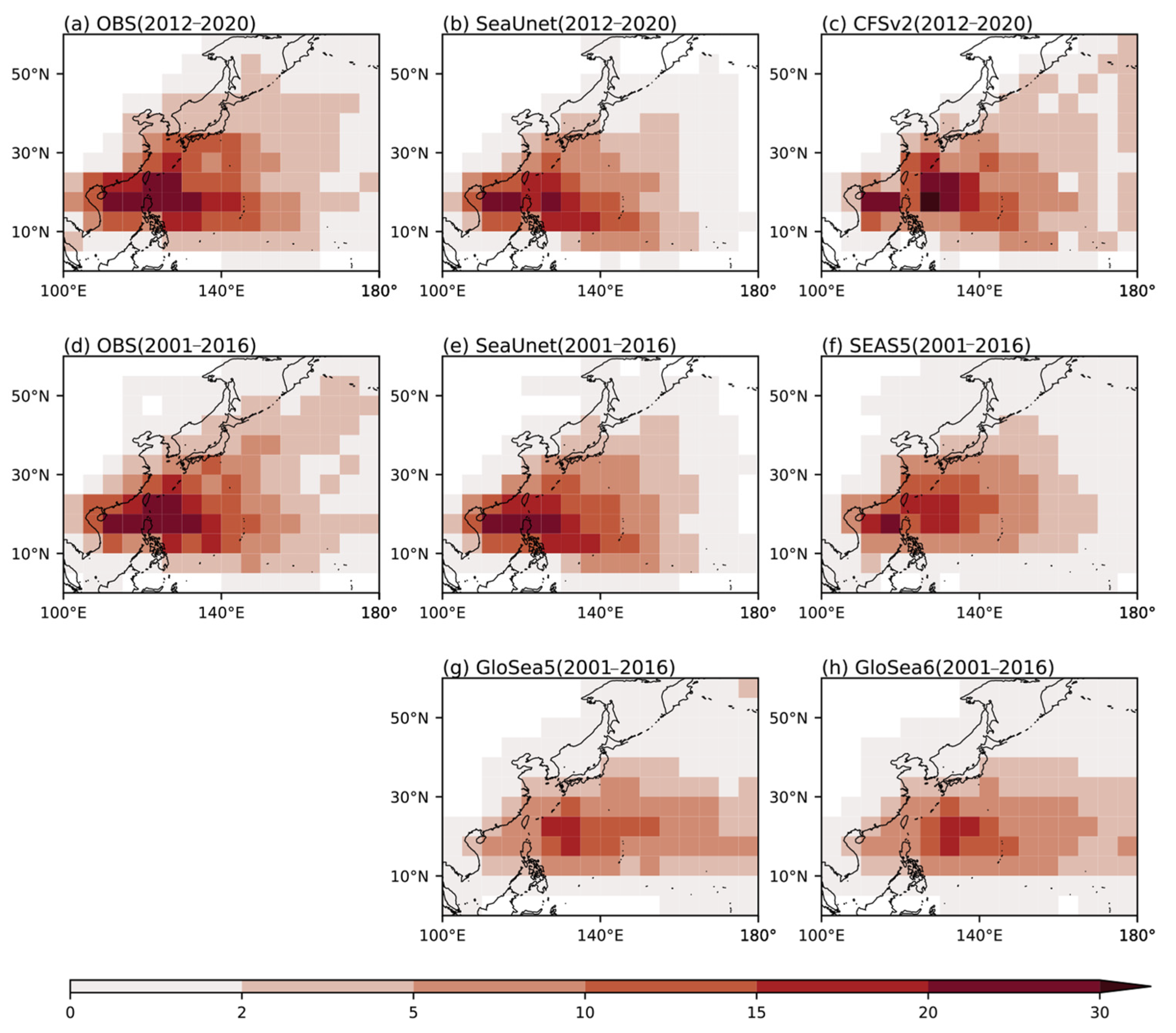
3.1. Climate-Mean Comparison

Figure 2 shows the climate mean predicted at the beginning of June for the WNP TC track density from June to November by SeaUnet and the four numerical models. Since the time range of the CFSv2 model is inconsistent with the other three numerical models, SeaUnet selects the period of 2012–2020 for comparison with the CFSv2 model. The time range is 2001–2016 for the other three models. This is due to the different time ranges of publicly available data. The observed WNP TC track density has the largest values around Taiwan and Luzon Island (Figure 2a,d). The SeaUnet can predict the large-value regions as observed. SeaUnet, CFSv2, and SEAS5 can well reproduce the key regions, while Glosea5 and Glosea6 only capture the large-value regions east of Luzon Island with lower values. The spatial correlation coefficients in TC track density between the models and the observation are 0.95 (SeaUnet, 2012–2020), 0.90 (CFSv2, 2012–2020), 0.97 (SeaUnet, 2001–2016), 0.96 (SEAS5, 2001–2016), 0.81 (Glosea5, 2001–2016), and 0.83 (Glosea6, 2001–2016). This indicates that the SeaUnet is the best, followed by SEAS5.

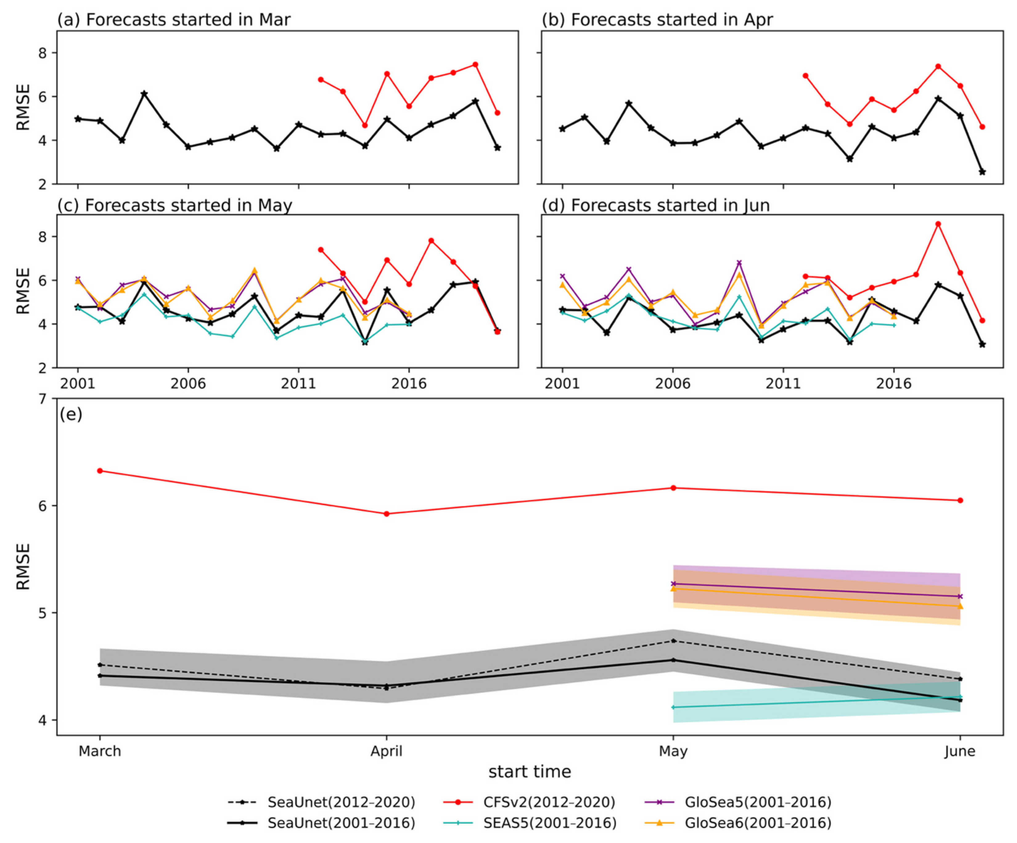
3.2. Year-by-Year Comparison

In routine operation, seasonal prediction focuses on year-to-year variability rather than the climate mean. In this study, area-averaged RMSE was used to evaluate the skills of each model in predicting annual TC track density. Figure 3a–d shows the year-by-year evolution of the area-averaged RMSE between the predicted TC track density and observations in different starting months. As SEAS5, Glosea5, and Glosea6 can only make predictions seven months in advance, only the prediction started in May and June can cover June–November (Figure 3c,d), while CFSv2 can provide June–November predictions in March (Figure 3a), which is why we chose CFSv2, even though it has a shorter available time period. In terms of RMSE, SeaUnet gave similar trends to the four numerical models. Moreover, SeaUnet’s prediction results are better than CFSv2′s for both March and April predictions (Figure 3a,b). Starting in May, SeaUnet’s prediction is worse than SEAS5′s (Figure 3c). But when starting in June, SeaUnet’s is significantly better than SEAS5′s, although in some years SeaUnet’s is worse than SEAS5′s. In addition, we evaluated our model using spatial correlation coefficients (Figure S5 in Supplementary Materials). As shown in Figure 3, SeaUnet is superior to CFSV2, Glosea5, and Glosea6 at all lead times. As in Ham et al. [28], the lead time is defined as the number of months between the latest available observation data and the start of the six-month prediction target period. Compared to SEAS5, however, the prediction skill of SeaUnet is a little lower in May.
To clearly show the evolution of the prediction errors of each model with different starting times, we designed Figure 3e. Except for the predictions started in May, the prediction error of SeaUnet becomes smaller with reduced lead time. However, this trend is not clear in the four numerical models. SeaUnet’s prediction started in May has the largest error, which also partly explains why SeaUnet in Figure 3c is weaker than those of the numerical models started in May. However, SeaUnet outperforms the other models in the other three start times (i.e., March, April and June). Note that SeaUnet has the best prediction skills in June, and wins with a small margin compared with SEAS5.

3.3. Physical Interpretation of SeaUnet Predictions

We used the heat map to interpret the physical meanings behind the SeaUnet predictions. SeaUnet’s main output (i.e., TC track density) is a network based on the fully convolutional network architecture. Currently, there are few studies on the interpretability of a fully convolutional network. Therefore, based on the main output network of SeaUnet, we added a secondary output to predict the aforementioned WNP TC track frequency (TCTF), which is the sum of the TC track density over a certain area (e.g., the WNP). The TCTF is not only related to the frequency of TC, but also to the TC duration. The predicted and observed WNP TCTFs from 2001 to 2016 were calculated (Figure 4a). By using H500, SubSST, and ushear in the boreal spring (using the MAM data) to train the SeaUnet, we show that SeaUnet can accurately predict the TCTF. The time correlation coefficient between the TCTF of SeaUnet prediction and observation reaches 0.67 and passes the 95% significance test. In second place is SEAS5, which also passes the 95% significance test with a correlation coefficient of 0.66. The correlation coefficients of Glosea5 and Glosea6 do not pass the 95% confidence test.
Through the heat map in the deep learning visualization, we analyzed the contributions of different regions to the WNP TCTF. Because of the characteristics of the heat map, the values of the shaded areas do not represent a positive or negative correlation, but only the relative contribution to the prediction of the WNP TCTF. For easy comparison, we calculated the normalized value of the heat map. We selected a minimum year (2010; Figure S3 in Supplementary Materials) and a maximum year (2018; Figure S3 in Supplementary Materials) for the heat map analysis. Note that year 2020 is also a minimum value year (Figure S3 in Supplementary Materials). Since the prediction error is large in 2020, we selected the second minimum value year (2010) with a smaller prediction error for the heat map analysis.
Although SeaUnet is an entirely data-driven statistical model, it can reveal certain physical processes using the heat map method. For example, there are three regions of high correlation in the tropical Pacific, tropical and subtropical Indian Ocean, South America, and in the pole in 2010 (Figure 4b); and two remarkable regions in the central and western tropical Pacific and Sea of Okhotsk in 2018 (Figure 4c). The high correlations of these regions with the WNP TCTF are also evident in the correlation coefficient map (Figure S4 in Supplementary Materials).
There is a highly negative correlation between the boreal-spring SST in the eastern Indian Ocean (75°–100°E, 10°S–22.5°N) and WNP TCTF, which may be related to the influence of the SST anomaly in the eastern Indian Ocean on the East Asian and western Pacific summer monsoons and equatorial Kelvin wave [38]. This region is also included in the Indian Ocean large-value region in Figure 4b. The SST gradient between the Indian Ocean and western Pacific warm pool in spring can cause low-level negative vorticity, strong vertical wind shear, and anticyclone anomalies at the low level in most areas of the WNP, favoring a reduction of TC occurrence frequency [39]. The Spring Indian Ocean Dipole (IOD) is also an important influencing factor. A positive SIOD can strengthen the WNP monsoon trough in summer, conducive to more TC genesis [40].
The highly correlated sea areas in the central tropical Pacific shown in Figure 4c are due to the development of the ENSO. There have been many studies on ENSO’s influence on WNP TC activities [41,42]. The temporal teleconnection between ENSO and WNP TC may be related to the fact that the climate anomalies caused by El Nino can continue into summer, which includes a warm SST over the tropical Indian Ocean, the warming of troposphere in the tropics, and the anticyclonic anomalies over the subtropical region of the WNP [43,44]. In addition to the ENSO, the sea-ice cover in spring near the Sea of Okhotsk and the Bering Sea shows significant negative correlations with the WNP SST, thus affecting the activity of WNP TCs [45]. This is also consistent with the high contribution areas in the mid and high latitudes in Figure 4c.
We used not only ocean thermal factors as predictors; some dynamic factors that can reflect large-scale circulations were also introduced into the model. Therefore, the heat map was not limited to thermal factors. For example, the high correlation region of the Southern Hemisphere’s subtropical regions, except the Atlantic Ocean (Figure 4b), may be related to the subtropical high (see Figure S4e,f in Supplementary Materials), and this mechanism may be linked to the influence of the Hadley circulation in boreal spring [46]. As a response to SST, the Arctic Oscillation (AO) associated with surface circulation in the Beaufort Sea [47] is also an important precursor signal to the WNP TC frequency during the boreal spring [48,49], which can be seen in Figure S4a–c in Supplementary Materials.
Due to the complexity of air–sea interactions, in some years some other factors may be dominant in determining the WNP TCTF, such as tropical North Atlantic SST anomalies in spring (Figure S4a–c in Supporting Information) [50,51], the SST gradient between the southwestern Pacific and western Pacific warm pool in spring (Figure S4c in Supporting Information) [52,53], northern Indian Ocean SSTs (Figure S4b in Supporting Information) [54], etc. The heat map analysis also indicates that some other areas, which were not investigated in previous studies on WNP TCs, contribute to the WNP TCTF. These areas also have a high incidence of some typical weather processes (e.g., Ural Mountains blocking high). Thereby, as an effective tool to solve nonlinear problems, the heat map provides a new way for us to study the mechanisms behind the WNP TC seasonal prediction.

4. Conclusions

Based on deep learning, we developed a new model for seasonal prediction of WNP TC track density, and proposed a method to study the nonlinear correlation between WNP TC activity and precursors by using a heat map [28,30]. The SeaUnet performs well in predicting the WNP TC track density, and characteristics of TC activity from June to November are predicted four months in advance. The area-averaged RMSE between the observed and SeaUnet-predicted WNP TC track density is smaller than that between the observed and predicted WNP TC track density given by the dynamic models, except at the start time in May (when the SeaUnet is only worse than SEAS5). However, SEAS5′s prediction is only two months in advance, whereas SeaUnet’s is four months in advance. Except for the predictions started in May, the prediction error of SeaUnet becomes smaller when the lead time becomes shorter. However, this trend is not clear in the results of the four numerical models. To explore the regions with significant contributions to the WNP TC activities, we used the heat map method. Due to the characteristics of the heat map, we predicted the WNP TCTF by using a secondary output of SeaUnet, which can reflect their frequency and life history. The correlation skill of the WNP TCTF can reach 0.67, which is better than the correlation skills of the other numerical models. The regions with significant contributions match well with the key regions identified by previous theoretical studies [39,40,41,45,48,49] and are consistent with the correlation analysis (Figure S4 in Supplementary Materials). The heat map was also used for regions with a high incidence of typical weather processes, which was not studied previously, such as the Ural Mountains blocking high. Different from traditional correlation and regression methods, the heat map is a highly nonlinear model, which provides a new research tool for us to study the seasonal prediction mechanism of WNP TC activity.
In this study, the main reasons for the better results of SeaUnet compared with the results of numerical models are as follows: (1) SeaUnet is a CNN-based fully convolutional neural network architecture, whose network backbone is ResUnet (a deep learning model based on residual connectivity). The strong feature representation of ResUnet allows it to show excellent performance in tasks such as image classification, which is appropriate for the prediction of TC track density; (2) SeaUnet uses a SE attention (Figure S1) module, which considers that channels of the feature map contribute differently to the task and assigns the corresponding weights. This attention mechanism allows the model to focus more on the most informative channel features and suppress those that are not important, which favors the improvement of forecast results; (3) The use of the transfer-learning method makes CMIP, as a pre-training dataset, greatly increase the training set samples, which in turn facilitates the convergence of the model and favors the improvement of forecast results.
Although, to some extent, the SeaUnet is better than the numerical models, further optimization of the model or adjustment of training strategy is needed. Although only the seasonal prediction of WNP TCs was carried out in this study, the advantage of the SeaUnet prediction also provides a good indication for other basins where TCs are active, e.g., the Indian Ocean and North Atlantic. We plan to carry out seasonal TC predictions in other ocean basins. We are also developing a unified prediction of TC track density distribution probability and TC frequency for operational prediction. In addition, part of the information shown in the heat map is consistent with previous theoretical analysis. Based on the nonlinear solution of the heat map, the influence of some unnoticed regions with significant contributions to TCs may need to be further studied in combination with numerical models.

Supplementary Materials

The following supporting information can be downloaded at: https://www.mdpi.com/article/10.3390/rs15071797/s1. Refs. [55,56,57,58] are cited in the Supplementary Materials.

Author Contributions

Conceptualization, Y.S. (Yuan Sun); methodology, Y.S. (Yuan Sun) and S.L.; software, Z.F. and S.L.; validation, P.Z., Y.S. (Yuan Sun) and Y.S. (Yixuan Shen); formal analysis, Z.F. and S.L.; investigation, Z.F. and S.L.; resources, Y.S. (Yuan Sun) and X.F.; data curation, Z.F. and S.L.; writing—original draft preparation, Z.F. and S.L.; writing—review and editing, Y.S. (Yuan Sun), Z.F. and S.L.; visualization, Z.F. and S.L.; supervision, Y.S. (Yuan Sun) and Y.L.; project administration, Y.S. (Yuan Sun); funding acquisition, Y.S. (Yuan Sun) and W.Z. All authors have read and agreed to the published version of the manuscript.

Funding

Please add: This research was supported by National Natural Science Foundation of China (Grants 42075035 and 42075011).

Data Availability Statement

SeaUnet’s parameters and prediction results: https://pan.baidu.com/s/1wjGb9Hh0HstLYaLcxPqlSw?pwd=4teo (accessed on 18 February 2023). IBTrACS: https://www.ncei.noaa.gov/products/international-best-track-archive?name=ib-v4-access (accessed on 6 January 2023). ERA5 single level variables: https://cds.climate.copernicus.eu/cdsapp#!/dataset/reanalysis-era5-single-levels-monthly-means (accessed on 13 January 2023). ERA5 pressure level variables: https://cds.climate.copernicus.eu/cdsapp#!/dataset/reanalysis-era5-pressure-levels-monthly-means (accessed on 13 January 2023). HadIOD: https://www.metoffice.gov.uk/hadobs/hadiod/download-hadiod1-2-0-0.html (accessed on 15 January 2023). CMIP6 and CMIP5: https://esgf-node.llnl.gov/projects/esgf-llnl/ (accessed on 9 January 2023). SEAS5, Glosea5 and Glosea6: https://cds.climate.copernicus.eu/cdsapp#!/search?type=dataset (accessed on 27 January 2023). CFSv2: https://www.ncei.noaa.gov/products/weather-climate-models/climate-forecast-system#CFSv2%20Operational%20Forecasts (accessed on 26 January 2023). SeaUnet’s Code: https://github.com/sure6963/wnp_tctd.git (accessed on 15 January 2023). The codes to identify TC: https://github.com/sure6963/identify-tc.git (accessed on 17 January 2023).

Acknowledgments

We thank Suzana J. Camargo (Columbia University) for providing the TC information of the CMIP5 models used in this study. We thank Zhong Zhong (National University of Defense Technology) for early discussions and advice on Methods. Zhihao Feng and Shuo Lv contributed equally to this work.

Conflicts of Interest

The authors declare no conflict of interest.

References

  1. Kim, D.; Kim, H.S.; Park, D.S.R.; Park, M.S. Variation of the tropical cyclone season start in the western north pacific. J. Clim. 2017, 30, 3297–3302. [Google Scholar] [CrossRef]
  2. Zhan, R.; Wang, Y.; Ying, M. Seasonal forecasts of tropical cyclone activity over the western North Pacific: A review. Trop. Cyclone Res. Rev. 2012, 1, 307–324. [Google Scholar]
  3. Li, R.C.Y.; Zhou, W. Modulation of western north pacific tropical cyclone activity by the ISO. Part I: Genesis and intensity. J. Clim. 2013, 26, 2904–2918. [Google Scholar] [CrossRef]
  4. Li, R.C.Y.; Zhou, W. Modulation of western North Pacific tropical cyclone activity by the ISO. Part II: Tracks and landfalls. J. Clim. 2013, 26, 2919–2930. [Google Scholar] [CrossRef]
  5. Zhao, H.; Wu, L.; Zhou, W. Interannual changes of tropical cyclone intensity in the western North Pacific. J. Meteorol. Soc. Jpn. 2011, 89, 243–253. [Google Scholar] [CrossRef] [Green Version]
  6. Wu, Q.; Wang, X.; Tao, L. Interannual and interdecadal impact of western north pacific subtropical high on tropical cyclone activity. Clim. Dyn. 2020, 54, 2237–2248. [Google Scholar] [CrossRef] [Green Version]
  7. Zhao, H.; Wang, C. On the relationship between ENSO and tropical cyclones in the western North Pacific during the boreal summer. Clim. Dyn. 2018, 52, 275–288. [Google Scholar] [CrossRef] [Green Version]
  8. Patricola, C.M.; Camargo, S.J.; Klotzbach, P.J.; Saravanan, R.; Chang, P. The Influence of ENSO flavors on western North Pacific tropical cyclone activity. J. Clim. 2018, 31, 5395–5416. [Google Scholar] [CrossRef]
  9. Zhan, R.; Wang, Y.; Zhao, J. Contributions of SST anomalies in the Indo-Pacific ocean to the interannual variability of tropical cyclone genesis frequency over the western North Pacific. J. Clim. 2019, 32, 3357–3372. [Google Scholar] [CrossRef]
  10. Yu, J.; Li, T.; Tan, Z.; Zhu, Z. Effects of tropical north Atlantic SST on tropical cyclone genesis in the western North Pacific. Clim. Dyn. 2016, 46, 865–877. [Google Scholar] [CrossRef]
  11. Hu, C.; Zhang, C.; Yang, S.; Chen, D.; He, S. Perspective on the northwestward shift of autumn tropical cyclogenesis locations over the western North Pacific from shifting ENSO. Clim. Dyn. 2018, 51, 2455–2465. [Google Scholar] [CrossRef] [Green Version]
  12. Zhao, J.; Zhan, R.; Wang, Y.; Xu, H. Contribution of the Interdecadal Pacific Oscillation to the recent abrupt decrease in tropical cyclone genesis frequency over the western North Pacific since 1998. J. Clim. 2018, 31, 8211–8224. [Google Scholar] [CrossRef]
  13. Klotzbach, P.; Blake, E.; Camp, J.; Caron, L.-P.; Chan, J.C.L.; Kang, N.-Y.; Zhan, R. Seasonal tropical cyclone forecasting. Trop. Cyclone Res. Rev. 2019, 8, 134–148. [Google Scholar] [CrossRef]
  14. Wang, C.; Wang, B. Tropical cyclone predictability shaped by western Pacific subtropical high: Integration of trans-basin sea surface temperature effects. Clim. Dyn. 2019, 53, 2697–2714. [Google Scholar] [CrossRef]
  15. Zhang, W.; Vecchi, G.A.; Villarini, G.; Murakami, H.; Gudgel, R.; Yang, X. Statistical–dynamical seasonal forecast of western North Pacific and east Asia landfalling tropical cyclones using the GFDL FLOR coupled climate model. J. Clim. 2017, 30, 2209–2232. [Google Scholar] [CrossRef] [Green Version]
  16. Wang, C.; Wang, B.; Wu, L. A region-dependent seasonal forecasting framework for tropical cyclone genesis frequency in the western North Pacific. J. Clim. 2019, 32, 8415–8435. [Google Scholar] [CrossRef]
  17. Murakami, H.; Vecchi, G.A.; Villarini, G.; Delworth, T.L.; Gudgel, R.; Underwood, S.; Yang, X.; Zhang, W.; Lin, S. Seasonal forecasts of major hurricanes and landfalling tropical cyclones using a high-resolution GFDL coupled climate model. J. Clim. 2016, 29, 7977–7989. [Google Scholar] [CrossRef]
  18. Li, J.; Bao, Q.; Liu, Y.; Wu, G.; Wang, L.; He, B.; Wang, X.; Li, J. Evaluation of FAMIL2 in simulating the climatology and seasonal-to-interannual variability of tropical cyclone characteristics. J. Adv. Model. Earth Syst. 2019, 11, 1117–1136. [Google Scholar] [CrossRef]
  19. Manganello, J.V.; Hodges, K.I.; Cash, B.A.; Kinter, J.L.; Altshuler, E.L., III; Fennessy, M.J.; Vitart, F.; Molteni, F.; Towers, P. Seasonal forecasts of tropical cyclone activity in a high-atmospheric-resolution coupled prediction system. J. Clim. 2016, 29, 1179–1200. [Google Scholar] [CrossRef]
  20. Feng, X.; Klingaman, N.P.; Hodges, K.I.; Guo, Y.P. Western North Pacific tropical cyclones in the Met Office global seasonal forecast system: Performance and ENSO teleconnections. J. Clim. 2020, 33, 10489–10504. [Google Scholar] [CrossRef]
  21. Camp, J.; Bett, P.E.; Golding, N.; Hewitt, C.D.; Mitchell, T.D.; Scaife, A.A. Verification of the 2019 GloSea5 seasonal tropical cyclone landfall forecast for east China. J. Meteorol. Res. 2020, 34, 917–925. [Google Scholar] [CrossRef]
  22. Zhang, W.; Villarini, G. Seasonal forecasting of western North Pacific tropical cyclone frequency using the North American multi-model ensemble. Clim. Dyn. 2019, 52, 5985–5997. [Google Scholar] [CrossRef]
  23. Zhang, G.; Murakami, H.; Gudgel, R.; Yang, X. Dynamical seasonal prediction of tropical cyclone activity: Robust assessment of prediction skill and predictability. Geophys. Res. Lett. 2019, 46, 5506–5515. [Google Scholar] [CrossRef]
  24. Chan, K.T.; Dong, Z.; Zheng, M. Statistical seasonal forecasting of tropical cyclones over the western North Pacific. Environ. Res. Lett. 2021, 16, 074027. [Google Scholar] [CrossRef]
  25. Palmer, T.N. Predictability of Weather and Climate: From Theory to Practice; Cambridge University Press: Cambridge, UK, 2006. [Google Scholar]
  26. Yu, S.; Ma, J. Deep learning for geophysics: Current and future trends. Rev. Geophys. 2021, 59, e2021RG000742. [Google Scholar] [CrossRef]
  27. Wimmers, A.; Velden, C.; Cossuth, J.H. 2019: Using deep learning to estimate tropical cyclone intensity from satellite passive microwave imagery. Mon. Weather Rev. 2019, 147, 2261–2282. [Google Scholar] [CrossRef]
  28. Ham, Y.G.; Kim, J.H.; Luo, J.J. Deep learning for multi-year ENSO forecasts. Nature 2019, 573, 568–572. [Google Scholar] [CrossRef] [PubMed]
  29. Kim, J.; Kwon, M.; Kim, S.D.; Kug, J.S.; Ryu, J.G.; Kim, J. Spatiotemporal neural network with attention mechanism for El Niño forecasts. Sci. Rep. 2022, 12, 7204. [Google Scholar] [CrossRef] [PubMed]
  30. Tang, Y.; Duan, A. Using deep learning to predict the East Asian summer monsoon. Environ. Res. Lett. 2021, 16, 124006. [Google Scholar] [CrossRef]
  31. Andersson, T.R.; Hosking, J.S.; Pérez-Ortiz, M.; Paige, B.; Elliott, A.; Russell, C.; Law, S.; Jones, D.C.; Wilkinson, J.; Phillips, T.; et al. Seasonal Arctic Sea ice forecasting with probabilistic deep learning. Nature. Commun. 2021, 12, 5124. [Google Scholar] [CrossRef]
  32. Liu, K.S.; Chan, J.C. Interdecadal variability of western North Pacific tropical cyclone tracks. J. Clim. 2008, 21, 4464–4476. [Google Scholar] [CrossRef]
  33. Rudzin, J.E.; Chen, S.; Sanabia, E.R.; Jayne, S.R. The air-sea response during Hurricane Irma’s (2017) rapid intensification over the Amazon-Orinoco River plume as measured by atmospheric and oceanic observations. J. Geophys. Res. Atmos. 2020, 125, e2019JD032368. [Google Scholar] [CrossRef]
  34. Liu, K.S.; Chan, J.C. Inactive period of western North Pacific tropical cyclone activity in 1998–2011. J. Clim. 2013, 26, 2614–2630. [Google Scholar] [CrossRef]
  35. Zhang, H.; Feng, L.; Zhang, X.; Yang, Y.; Li, J. Necessary conditions for convergence of CNNs and initialization of convolution kernels. Digit. Signal Process. 2022, 123, 103397. [Google Scholar] [CrossRef]
  36. Pang, S.; Xie, P.; Xu, D.; Meng, F.; Tao, X.; Li, B.; Li, Y.; Song, T. NDFTC: A New Detection Framework of Tropical Cyclones from Meteorological Satellite Images with Deep Transfer Learning. Remote Sens. 2021, 13, 1860. [Google Scholar] [CrossRef]
  37. Zhou, B.; Khosla, A.; Lapedriza, A.; Oliva, A.; Torralba, A. Learning deep features for discriminative localization. In Proceedings of the 2016 IEEE Conference on Computer Vision and Pattern Recognition (CVPR), Las Vegas, NV, USA, 27–30 June 2016; pp. 2921–2929. [Google Scholar]
  38. Zhan, R.; Wang, Y.; Lei, X. Contributions of ENSO and east Indian ocean SSTA to the interannual variability of northwest Pacific tropical cyclone frequency. J. Clim. 2011, 24, 509–521. [Google Scholar] [CrossRef]
  39. Wang, L.; Chen, G. Impact of the spring SST gradient between the tropical Indian ocean and western Pacific on landfalling tropical cyclone frequency in China. Adv. Atmos. Sci. 2018, 35, 682–688. [Google Scholar] [CrossRef]
  40. Zhou, Q.; Zhang, R. Possible impacts of spring subtropical Indian Ocean Dipole on the summer tropical cyclone genesis frequency over the western North Pacific. Int. J. Climatol. 2022, 42, 5393–5402. [Google Scholar] [CrossRef]
  41. Wang, B.; Chan, J.C. How strong ENSO events affect tropical storm activity over the western North Pacific. J. Clim. 2002, 15, 1643–1658. [Google Scholar] [CrossRef]
  42. Du, Y.; Yang, L.; Xie, S.P. Tropical Indian Ocean influence on northwest Pacific tropical cyclones in summer following strong El Niño. J. Clim. 2011, 24, 315–322. [Google Scholar] [CrossRef]
  43. Xie, S.P.; Hu, K.; Hafner, J.; Tokinaga, H.; Du, Y.; Huang, G.; Sampe, T. Indian Ocean capacitor effect on Indo–western Pacific climate during the summer following El Niño. J. Clim. 2009, 22, 730–747. [Google Scholar] [CrossRef]
  44. Xie, S.P.; Kosaka, Y.; Du, Y.; Hu, K.; Chowdary, J.S.; Huang, G. Indo-western Pacific ocean capacitor and coherent climate anomalies in post-ENSO summer: A review. Adv. Atmos. Sci. 2016, 33, 411–432. [Google Scholar] [CrossRef] [Green Version]
  45. Fan, K. North Pacific sea ice cover, a predictor for the western North Pacific typhoon frequency? Sci. China Ser. D Earth Sci. 2007, 50, 1251–1257. [Google Scholar] [CrossRef]
  46. Zhou, B.T.; Cui, X. Modeling the influence of spring Hadley circulation on the summer tropical cyclone frequency in the western North Pacific. Chin. J. Geophys. 2009, 52, 1231–1236. [Google Scholar] [CrossRef]
  47. Armitage, T.W.; Bacon, S.; Kwok, R. Arctic sea level and surface circulation response to the Arctic Oscillation. Geophys. Res. Lett. 2018, 45, 6576–6584. [Google Scholar] [CrossRef]
  48. Cao, X.; Chen, S.; Chen, G.; Chen, W.; Wu, R. On the weakened relationship between spring Arctic Oscillation and following summer tropical cyclone frequency over the western North Pacific: A comparison between 1968-1986 and 1989-2007. Adv. Atmos. Sci. 2015, 32, 1319–1328. [Google Scholar] [CrossRef]
  49. Choi, K.S.; Wu, C.C.; Byun, H.R. Possible connection between summer tropical cyclone frequency and spring Arctic Oscillation over East Asia. Clim. Dyn. 2012, 38, 2613–2629. [Google Scholar] [CrossRef]
  50. Zuo, J.; Li, W.; Sun, C.; Ren, H.C. Remote forcing of the northern tropical Atlantic SST anomalies on the western North Pacific anomalous anticyclone. Clim. Dyn. 2018, 52, 2837–2853. [Google Scholar] [CrossRef]
  51. Cao, X.; Chen, S.; Chen, G.; Wu, R. Intensified impact of northern tropical Atlantic SST on tropical cyclogenesis frequency over the western North Pacific after the late 1980s. Adv. Atmos. Sci. 2016, 33, 919–930. [Google Scholar] [CrossRef]
  52. Zhao, J.; Zhan, R.; Wang, Y.; Tao, L. Intensified interannual relationship between tropical cyclone genesis frequency over the northwest Pacific and the SST gradient between the southwest Pacific and the western Pacific warm pool since the mid-1970s. J. Clim. 2016, 29, 3811–3830. [Google Scholar] [CrossRef]
  53. Zhan, R.; Wang, Y.; Wen, M. The SST gradient between the southwestern Pacific and the western Pacific warm pool: A new factor controlling the northwestern Pacific tropical cyclone genesis frequency. J. Clim. 2013, 26, 2408–2415. [Google Scholar] [CrossRef] [Green Version]
  54. Wu, S.; Zhou, G. Relationship between sea surface temperature of middle–high latitude Indian ocean and summer typhoon frequencies over the western North Pacific. Clim. Environ. Res. 2013, 18, 243–250. [Google Scholar]
  55. Camargo, S.J.; Zebiak, S.E. Improving the detection and tracking of tropical cyclones in atmospheric general circulation models. Weather Forecast. 2002, 17, 1152–1162. [Google Scholar] [CrossRef]
  56. Sun, Y.; Zhong, Z.; Li, T.; Yi, L.; Hu, Y.; Wan, H.; Chen, H.; Liao, Q.; Ma, C.; Li, Q. Impact of ocean warming on tropical cyclone size and its destructiveness. Sci. Rep. 2017, 7, 8154. [Google Scholar] [CrossRef] [PubMed] [Green Version]
  57. Kim, D.; Jin, C.S.; Ho, C.H.; Kim, J.; Kim, J.H. Climatological features of WRF-simulated tropical cyclones over the western North Pacific. Clim. Dyn. 2015, 44, 3223–3235. [Google Scholar] [CrossRef]
  58. Song, K.; Yang, G.; Wang, Q.; Xu, C.; Liu, J.; Liu, W.; Shi, C.; Wang, Y.; Zhang, G.; Yu, X.; et al. Deep learning prediction of incoming rainfalls: An operational service for the city of Beijing China. In Proceedings of the 2019 International Conference on Data Mining Workshops (ICDMW), Beijing, China, 8–11 November 2019; pp. 180–185. [Google Scholar]
Figure 1. Schematic diagram of the SeaUnet network structure.
Remotesensing 15 01797 g001
Figure 2. Climate mean of WNP TC track density from June to November predicted in June. (a) Observation for the time range of 2012–2020; (b) predicted by SeaUnet; (c) predicted by CFSv2 for the time range of 2012–2020; (d) observation for the time range of 2001–2016; (e) predicted by SeaUnet; (f) predicted by SEAS5; (g) predicted by Glosea5; (h) predicted by Glosea6 for the time range of 2001–2016.
Remotesensing 15 01797 g002
Figure 3. Area-averaged root-mean-square error (RMSE) between predicted TC track density results. Annual RMSE of the predicted TC track density of SeaUnet, SEAS5, Glosea5, and Glosea6 ensemble mean with respect to the observation in different starting months (i.e., (a) start in March; (b) start in April; (c) start in May; and (d) start in June), with SeaUnet for the time range from 2001 to 2020, CFSv2 for the time range from 2012 to 2020, SEAS5, Glosea5, and Glosea6 for the time range from 2001 to 2016. (e) RMSE of each model changing with starting time. The solid line represents the average error of the ensemble mean of each model in the selected year, and the shading represents the 25% variance of the ensemble members. To ensure the rationality of comparison, the time range of the solid line for SeaUnet is from 2001 to 2016, and the time range of the dotted line is from 2012 to 2020; the time range for CFSv2 is from 2012 to 2020; and the time range for SEAS5, Glosea5, and Glosea6 is from 2001 to 2016.
Remotesensing 15 01797 g003
Figure 4. Physical interpretation of SeaUnet model TCTF predictions. (a) WNP TCTF predicted by the four models and observations from 2001 to 2016. The number after the colon in the legend represents the correlation coefficient between the predicted and observed values. Note that the lines of the three numerical models (SEAS5, GloSea5, and GloSea6) indicate their ensemble mean (see Table S1 in Supplementary Materials). (b) The heat map of 2010. (c) The heat map of 2018. The results are predicted by the SeaUnet with boreal-spring subsurface SST of the UK Met Office, using H500 and vertical shear of the u component of wind of the ERA5 data as the predictors.
Remotesensing 15 01797 g004
Disclaimer/Publisher’s Note: The statements, opinions and data contained in all publications are solely those of the individual author(s) and contributor(s) and not of MDPI and/or the editor(s). MDPI and/or the editor(s) disclaim responsibility for any injury to people or property resulting from any ideas, methods, instructions or products referred to in the content.

