Communication

A New Method for False Alarm Suppression in Heterogeneous Change Detection

1
School of Information and Communication Engineering, University of Electronic Science and Technology of China, Chengdu 611731, China
2
Department of Electrical and Information Engineering, Heilongjiang Institute of Engineering, Harbin 150026, China
*
Author to whom correspondence should be addressed.
Remote Sens. 2023, 15(7), 1745; https://doi.org/10.3390/rs15071745
Submission received: 19 February 2023 / Revised: 13 March 2023 / Accepted: 20 March 2023 / Published: 24 March 2023

Abstract

:
Heterogeneous change detection has a wide range of applications in many fields. However, to date, many existing problems of heterogeneous change detection, such as false alarm suppression, have not been specifically addressed. In this article, we discuss the problem of false alarm suppression and propose a new method based on the combination of a convolutional neural network (CNN) and graph convolutional network (GCN). This approach employs a two-channel CNN to learn the feature maps of multitemporal images and then calculates difference maps of different scales, which means that both low-level and high-level features contribute equally to the change detection. The GCN, with a newly built convolution kernel (called the partially absorbing random walk convolution kernel), classifies these difference maps to obtain the inter-feature relationships between true targets and false ones, which can be represented by an adjacent matrix. We use pseudo-label samples to train the whole network, which means our method is unsupervised. Our method is verified on two typical data sets. The experimental results indicate the superiority of our method compared to some state-of-the-art approaches, which proves the efficacy of our method in false alarm suppression.

Graphical Abstract

1. Introduction

Recently, heterogeneous change detection has drawn increased attention. Heterogeneous change detection aims to achieve change detection from images coming from different types of sensors. Its advantages over homogeneous change detection are clear. It not only combines the characteristics of multiple types of data and removes the environmental conditions. Additionally, it provides a timely change analysis, especially in case of disasters. However, many issues related to heterogeneous change detection have not been addressed, such as false alarms. False alarms can lead researchers to misjudge and mispredict the development trends of events. Furthermore, they can cause researchers to waste resources when dealing with change. Therefore, in this paper, we discuss the issue of false alarm suppression in detail.
Existing heterogeneous change detection methods can be classified from different perspectives. According to the availability of labeled samples, this type of detection can be classified into supervised and unsupervised methods. Since it is difficult to obtain change samples and ground truth maps, unsupervised methods are preferable to supervised ones. According to the processing scale, there are patch-level, pixel-level and subpixel-level methods. Among them, subpixel-level methods are more prominent in improving accuracy [1]. In [2], fine spatial but coarse temporal resolution images and coarse spatial but fine temporal images are combined to detect changes by using spectral unmixing to generate the abundance image. According to the principle of the algorithms, there are classification-based, parametric, non-parametric, similarity-based and translation and projection-based methods. Classification-based techniques compare the results of classifying individual images. Parametric techniques use a set of multivariate distributions to model the joint statistics of different imaging modalities, while non-parametric ones do not explicitly assume a specific parametric distribution. The similarity measures are modality-invariant properties. Translation or projection-based methods convert multimodal images onto a common space in which homogeneous change detection methods can be applied [3].
Among these methods, those based on translation and projection without the presupposition of various conditions have gained the greatest popularity. Non-deep learning methods and deep learning methods are used to realize translation and projection. First, we take a look at the non-deep learning methods. Based on changes in smoothness, a decomposition method was proposed to decompose the post-event image into a regression image of pre-event image and a changed image [4]. In [5], heterogeneous change detection was converted into a graph signal processing problem and structural differences were used to detect changes. In [6], a robust K-nearest neighbor graph was established and an iterative framework was put forward based on a combination of difference map generation and change map calculation. In [7], a self-expressive property was exploited and difference image was obtained by measuring how much one image conformed to the similarity graph compared to the other image. Furthermore, considering the impact of noise, the fusion of forward and backward difference images was accomplished by statistical modeling in [8]. In [9], a new method called INLPG was developed by constructing a graph for the whole image and applying the discrete wavelet transform to fuse difference images. In [10], a probabilistic graph was constructed and image translation was based on the sparse-constrained image regression model. Next, we investigated deep learning methods. A conditional generative adversarial network was used to transform the heterogeneous synthetic aperture radar (SAR) and optical images into the same space to form the difference image [11]. In [12], CycleGAN was adopted to translate the pre-event SAR image into an optical image, and the difference image was obtained by comparing the translated optical image with the post-event optical image. In [13], a self-supervised detection method was developed based on pseudo-training from affinity matrices and four kinds of regression methods, namely, Gaussian process regression, support vector regression, random forest regression, and homogeneous pixel transformation. In [14], two new convolutional neural networks were constructed with a loss function based on the affinity priors to mitigate the impact of change pixels on the learning objective. In [15], a graph fusion framework for change detection was proposed on the condition of smoothness priors. In [16], an end-to-end framework of a graph convolutional network was constructed to increase localization accuracy in the vertex domain by exploiting intra-modality and cross-modality information.
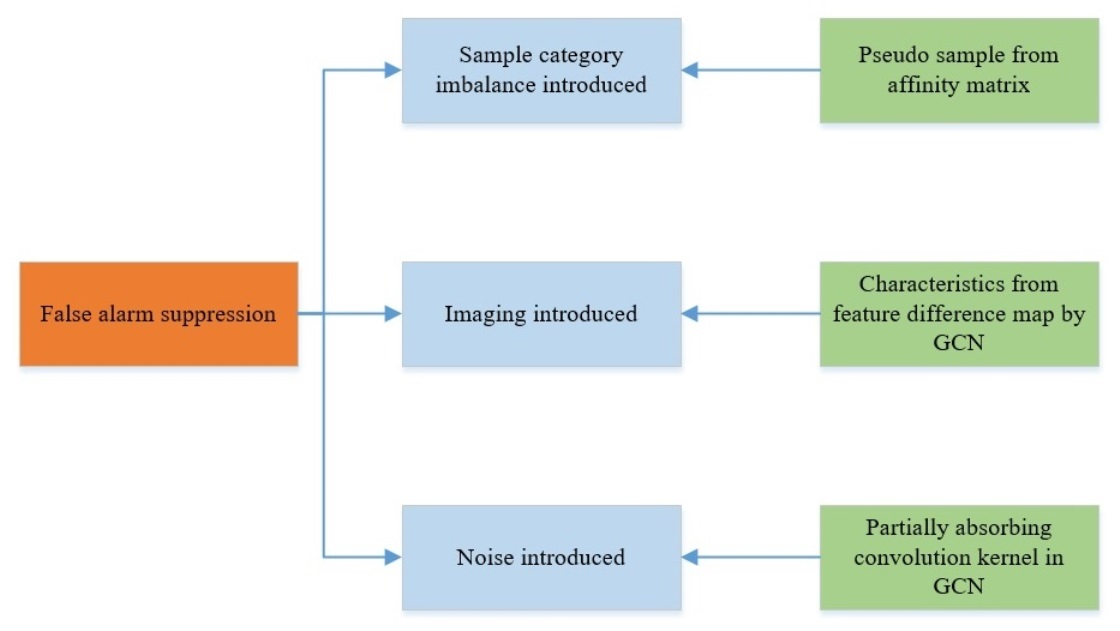
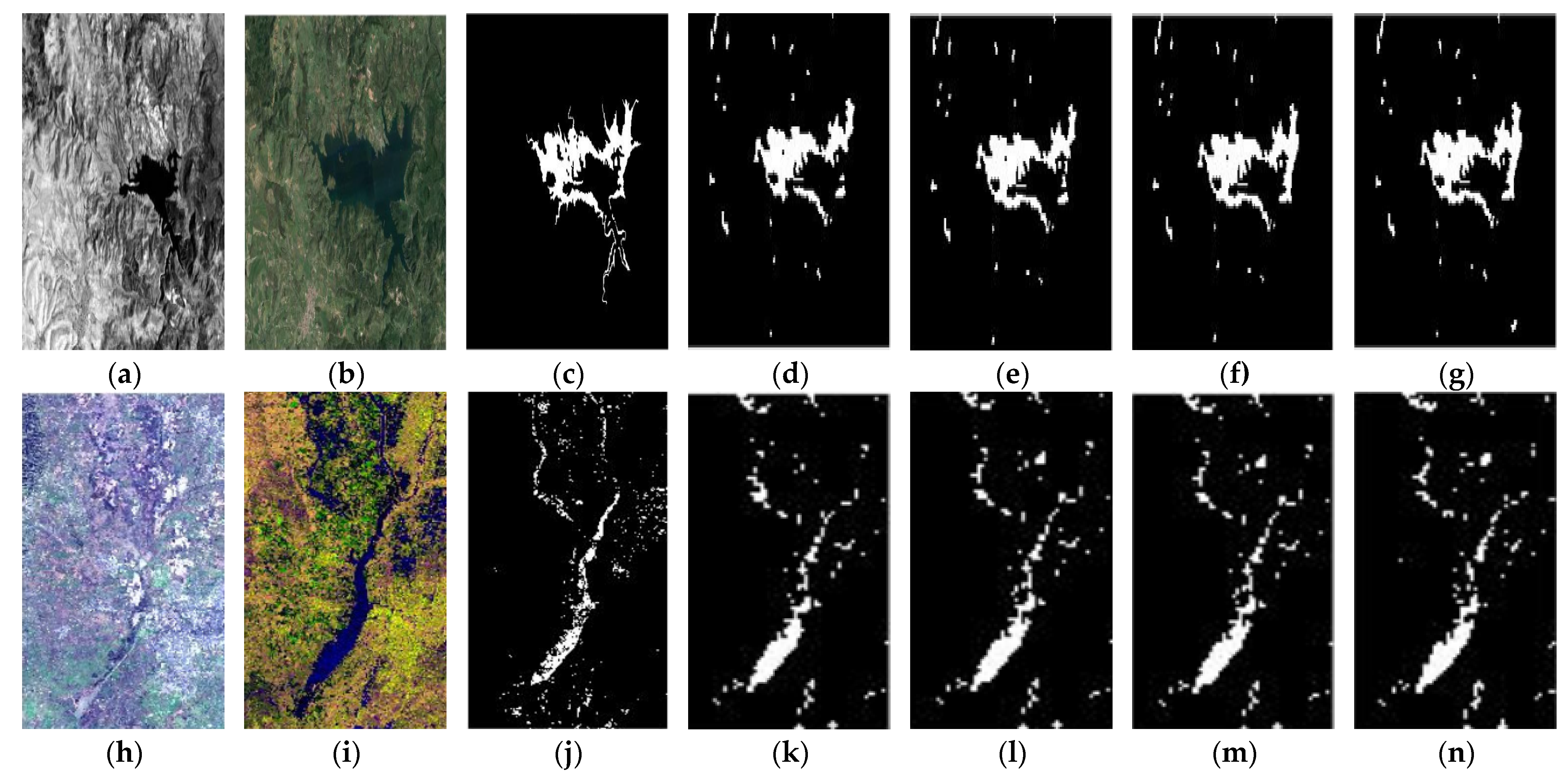
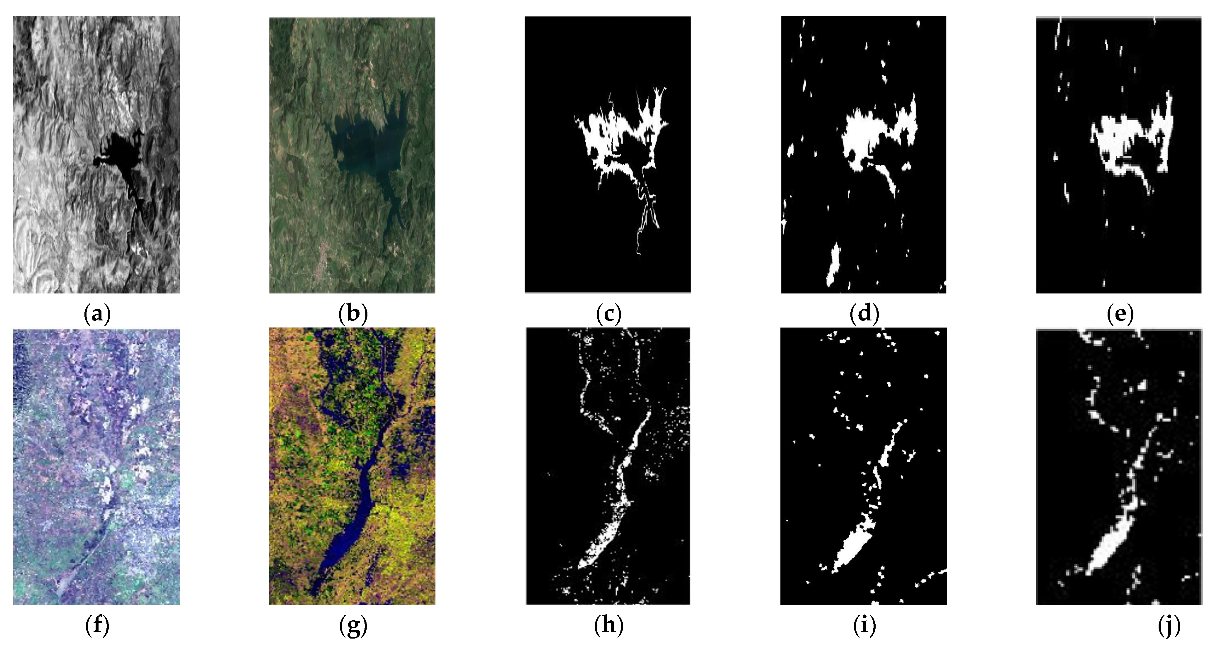
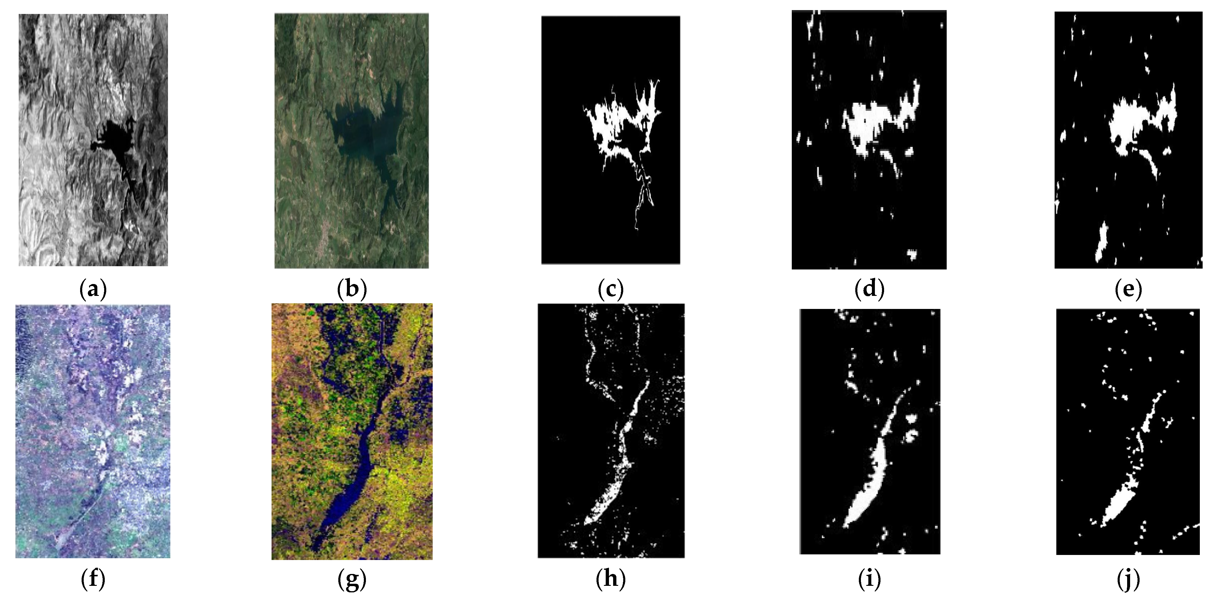
Generally, the detection results contain many pseudo-changes, which stem from three sources. The first is the difference between shapes and sizes of the same object in heterogeneous images, the second is the imbalance in sample categories in supervised and self-supervised methods, and the third is inherent noise in the imaging process. A common method to solve this problem is supervised classification, which requires some prior knowledge. In [17], a simple CNN was built to classify the feature difference maps with a few pixel-level training samples to suppress false alarms. In [18], a structural consistency loss based on the cross-modal distance between affinity and an adversarial loss were introduced to deal with pseudo-changes. In addition, a multitemporal segmentation combining the spectral, spatial, and temporal information of the heterogeneous images was introduced in the preprocessing to reduce false positives [19]. In [20], a feature difference network was built to reduce false detections by addressing the information loss and imbalance in feature fusion.
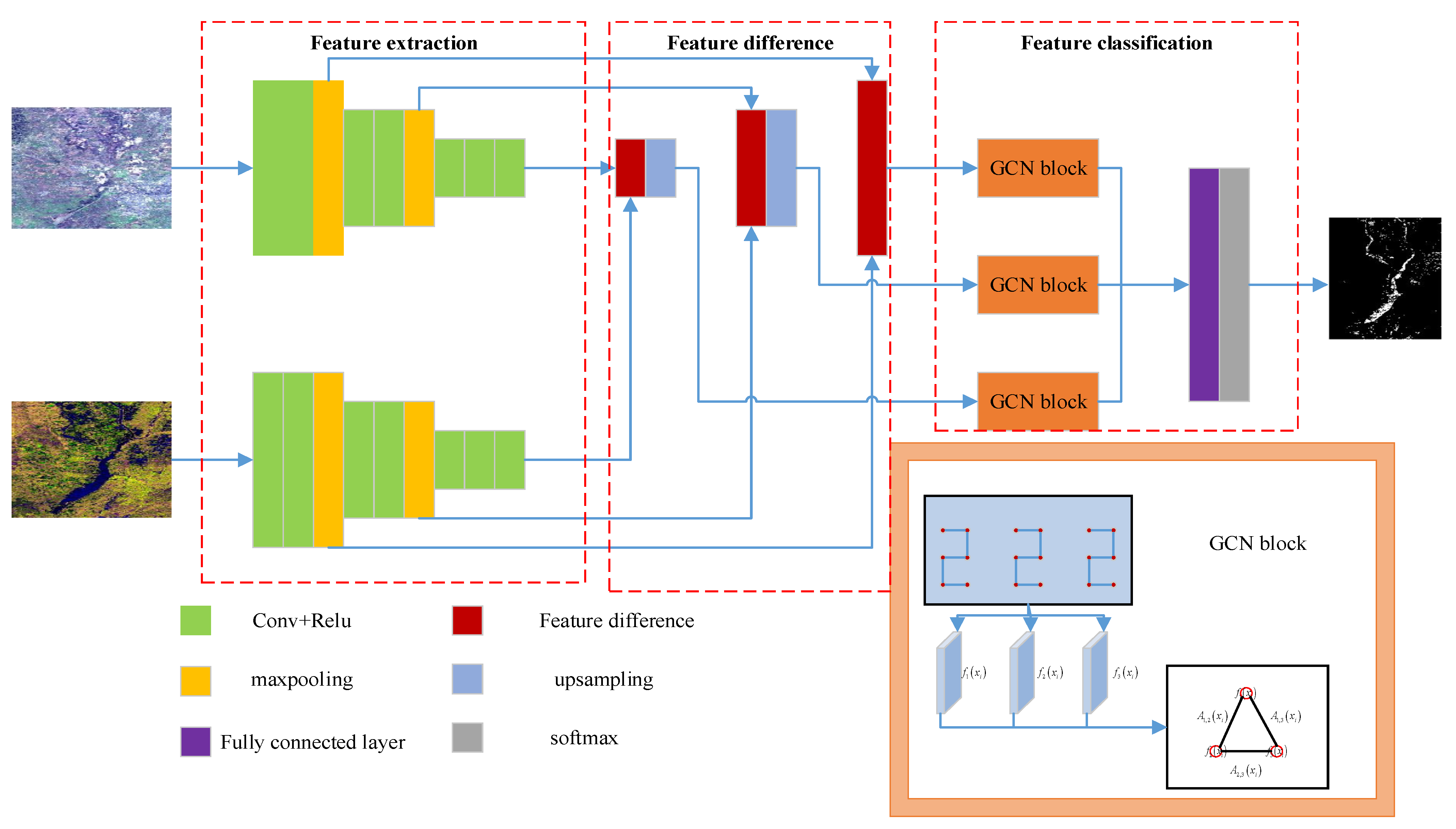
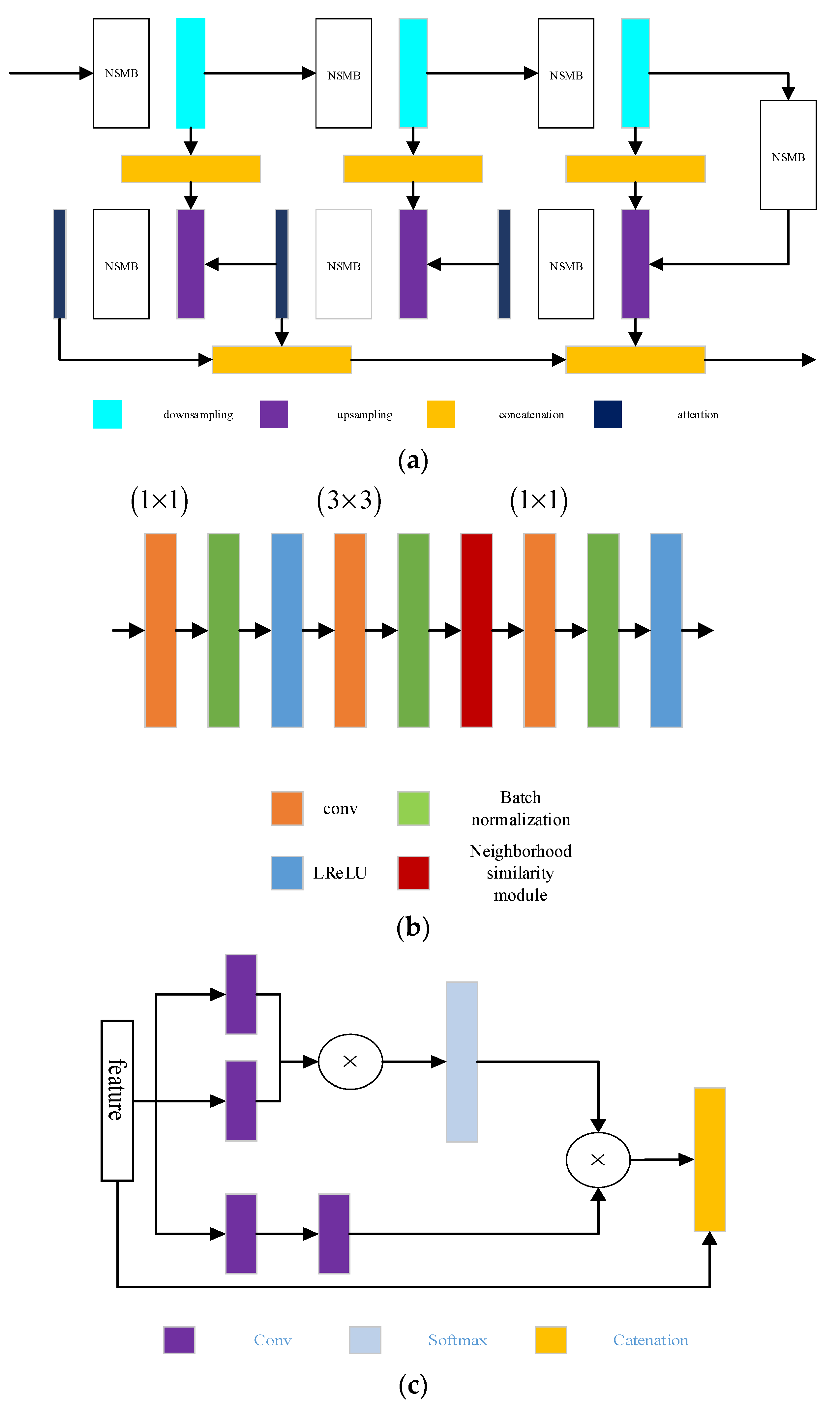
In this article, we propose a new method based on a combination of CNN and GCN to deal with false alarm suppression in heterogeneous change detection. The main contributions of our method are as follows: First, by generating pseudo-label samples to train the whole network, our method is unsupervised. This can help to avoid the false alarms introduced by imbalances in training sample categories. Second, we use the inter-feature relationships between true targets and false ones, which can be represented by an adjacent matrix to generate a change map. This can facilitate the detection of the same object, showing differences in the shapes and sizes of heterogeneous images. Third, a partially absorbing random walk convolution kernel is constructed and applied in the GCN. This new convolution kernel can enhance the features of individual vertex and mitigate the impact of noise to some extent, which is advantageous in the suppression of noise-introduced false alarms. This paper is organized as follows: Section 2 presents our proposed method and the experiment results obtained by comparison with some state-of-the-art approaches. Our final conclusion is given in Section 3.

2. Method

2.1. Generation of Pseudo-Label Samples

Two images, acquired at the same region by different sensors at different times, t 1 and t 2 , are denoted as X R n 1 × n 2 × p and Y R n 1 × n 2 × q , respectively, where n 1 and n 2 are the height and width, and p and q are the numbers of channels [13].
We aimed to develop a training set T = { ( x m , y m ) } m = 1 N , N < N , where N = n 1 × n 2 . A pair of corresponding patches were selected over the same area z between X and Y . The patches covered a k × k window, whose pixel i was denoted as z i l , where l indicates either X or Y . The distance d ( z i l , z j l ) was calculated between all pixel pairs in the patch by Euclidean distance.
These distances can be transformed to affinities as
A i , j l = exp { d ( z i l , z j l ) h 2 }
where h is determined as the mean of the seventh nearest neighbor for all the data in z l .
Since the affinity matrices indicate the spatial structure and relations between pixels in each patch, if there are changes, a large divergence between them will emerge. The distance between affinity matrices was calculated as
f = A X A Y
Each pixel is the average distance between the patches covering that pixel. We chose the pixels with a short average distance, which means these pixels come from the unchanged area. Then, we calculated the Euclidean distance between these pixels in the pre-event and after-event images separately. Finally, we chose the pixels with small Euclidean distances in both pre-event and after-event images as training samples. This is because the farther the pixels are, the more likely they are to have come from different categories.

2.2. Structure of Network

The principle of our method is illustrated in Figure 1. It includes three parts, namely, feature extraction, feature difference, and feature classification. In feature extraction, we apply CNN to extract the low- to high-level features of the pre-event image and after-event image. In feature difference, these features undergo difference processing, and feature difference maps are obtained. In feature classification, three difference maps enter separate GCN blocks to generate the inter-relationship features, and a fully connected layer is used to classify these features to generate a change map. The detailed structure of our network is illustrated in Table 1.
(1)
Feature extraction: since VGG16 is a lightweight CNN based network, the feature extraction net employed VGG16 as the backbone to separately extract the pre-event image and after-event image features. VGG16 includes 13 convolutional layers, 5 max pooling layers, and 3 fully connected layers. Here, VGG16 is pruned, and only the 2nd, 4th, and 7th convolutional layers were used.
(2)
Feature difference: since feature maps can reflect the changes in change detection task and difference maps of different scales can make both low-level and high-level features contribute equally to the change detection, we chose to add a feature difference module in our network. After obtaining individual feature maps of layer 2nd, 4th, and 7th, we generate their difference maps separately.
(3)
Feature classification: it is believed that differences in inter-feature relationships exist between true targets and false ones, which can be represented by an adjacent matrix A m . So, we apply the adjacent matrix A m as features. Since graph convolution tends to homogenize the features of different nodes, the number of layers in GCN was set to 3 in our proposed method. The intermediate feature maps of different levels in GCN are denoted by f m ( x n ) , where x n is the feature of pixel n , extracted from the m level. A new graph can be formed, with f m ( x n ) being the nodes and A m , p ( x n ) being the edge. A m , p ( x n ) was calculated as the Euclidean distance between f m ( x n ) and f p ( x n ) . After obtaining the features of A m , p ( x n ) , we deployed a fully connected layer to classify them and, finally, a change map is generated.
(4)
Partially absorbing random walk convolution kernel: in GCN, we introduced a newly built convolution kernel, which is enlightened by [21]. It was built by applying a partially absorbing random walk to graphs, which can find the most related vertices in the whole structure to maximize the feature of the vertex under concern and suppress noise.
The adjacency matrix can be expressed as
S = H ( D e I ) 1 H T D i a g ( H ( D e I ) 1 H T )
where H denotes the incidence matrix, and D e is a diagonal matrix of edge degrees.
Random walk on a graph can be formulated as
P = D v 1 S
where D v is a diagonal matrix of vertex degrees.
The corresponding Laplacian matrix is given as
L = D v S
Introducing a regularization matrix Λ = d i a g ( λ 1 , λ 2 , , λ N ) , and let C to be a absorption probability matrix,
C = ( Λ + L ) 1 Λ
There is Λ = α I , so we can obtain
C = ( α I + L ) 1 α
The convolution operator is defined as
Z ( l + 1 ) = σ ( C Z ( l ) Θ ( l ) )
where Z ( l ) is the l t h layer, Θ ( l ) is the parameter of the l t h layer, and C is formulated as
C = ( α I + L ) 1 α
where I is the identity matrix, L is the Laplacian matrix, and α is a predefined parameter.

2.3. Simulation

In this section, we conducted experiments on two different data sets to prove the efficacy of our proposed method. First, the data sets are presented. Then, quantitative measures are provided. Finally, the performance of our method is analyzed by comparison with some state-of-the-art methods.

2.3.1. Data Set Description

We used two typical data sets to verify our method. The Italy data set includes one near-infrared band image and one optical image, taken over Sardinia, Italy in September, 1995 and July, 1996, respectively [3]. The former derives from Landsat-5 and the latter from Google Earth with R, G, and B bands. The multitemporal images indicate the event of lake expansion, with a resolution of 30 m. The California data set includes a multispectral image, with eight channels taken by Landsat 8, and an SAR image with VV and VH polarizations taken over California on 5 January 2017, and 18 February 2017. The multitemporal images indicate a flood in this area [20]. The description of this data set is given in Table 2.

2.3.2. Quantitative Measures

We evaluated the performance of our method from two perspectives, namely, difference image (DI) generation and change map (CM) classification. DI was evaluated by the receiver-operating characteristics (ROC) curve, which plots the false positive against the true positive. The area under the curve (AUC) represents the performance, ranging from 0 to 1. The larger the AUC, the better the detection performance. The false alarm rate (FA) was also adopted to indicate the performance of false alarm suppression. CM was evaluated by overall accuracy (OA), Kappa coefficient (KC) and F1-score. OA was the ratio of correct classification pixels versus total pixels, ranging from 0 to 1. Kappa coefficient demonstrates the agreement between two classifiers, ranging from −1 to 1, which is calculated as
K C = P C C P R E 1 P R E
where
PRE = ( T P + F N ) ( T P + F P ) + ( T N + F P ) ( T N + F N ) ( T P + T N + F P + F N ) 2
T P , T N , F N and F P represent true positive, true negative, false negative and false positive, respectively.
F1-score is defined as
F 1 = T P T P + 1 2 ( F P + F N )

2.3.3. Performance Analysis

Our method was implemented on Tensorflow 2.1.0 with python. The inputs of our network were images of 224 × 224 pixels. The learning rate, momentum, and weight decay were set as 1 × 10⁻⁷, 0.99 and 0.0005, respectively.
To prove the superiority of our method, we selected another two methods, namely, FDCNN [4] and INLPG [17], and our method without the newly built convolution kernel for comparison. Instead of quoting the results in the original papers, we ran them under the same circumstances as our method and the results are shown in Figure 2, Table 3 and Table 4. Here, our method achieved a competitive detection ability with the other three methods and a better false alarm suppression ability than the other three methods. Among these four methods, INLPG was not effective in dealing with pseudo-changes. Both FDCNN and our method without a newly built convolution kernel showed a comparable performance in terms of false alarm suppression, which was better than INLPG. This is because they can eliminate the false alarms introduced by imaging conditions or surface color changes to some extent. Since our method, with a newly built convolution kernel, could not only mitigate the impact of imaging conditions or surface color changes, but also reduce noise influence, it showed the best overall performance regarding false alarm suppression.
In addition, we discuss the impact of predefined parameter α on the performance of our method, and the result is shown in Figure 3. Too small α could cause the probability to be distributed evenly on the whole graph, leading to the confusion of neighborhood vertices. Too large α could cause the probability to concentrate on a single vertex, leading to the ineffectiveness of convolution. When α was set properly, a vertex could aggregate the features in its neighborhood, so as to improve the classification performance. Therefore, α was set as 60 in our experiment.

2.3.4. Ablation Study

Two ablation experiments were conducted. One was to prove the effectiveness of the feature classification module. The other one was to show the effectiveness of VGG16 in feature extraction.
In the first experiment, we eliminated the feature classification module by replacing it with a CNN-based classifier, as in [17], and compared it with our proposed method (without a new convolution kernel). In the following, our proposed method referred to that without a new convolution kernel. The experiment results are shown in Figure 4 and Table 5 and Table 6, which all prove the effectiveness of our proposed method in false alarm suppression.
In the second experiment, we chose a network with the best performance among our self-constructed structures. The details of our self-constructed structure are shown in Figure 5. Accordingly, the feature difference module was pruned to be one layer and the feature classification module was eliminated and replaced by a CNN-based classifier as in [17]. Meanwhile, the feature classification module was eliminated and replaced by a CNN-based classifier as in [17] and our proposed method. The results are shown in Figure 6 and Table 7 and Table 8. From the experiment results, it was obvious that the feature extraction module in our proposed method was superior to our self-constructed one both in lightweight structure and detection performance.

3. Conclusions

In this paper, we focused on false alarm suppression in heterogeneous change detection. Our proposed method exploits the inherent features of pre-event and after-event images. We made the following innovations in our proposed method. First, we generated pseudo-label samples without sample imbalances to train our network, which meant our method was unsupervised. Second, we exploited inter-feature relationships to discriminate true changes and false ones by combining CNN and GCN. Third, we employed a new convolution kernel to mitigate the impact of noise. Our work is very enlightening, as false alarm suppression in heterogeneous change detection is rarely studied. We tested our method on different scenarios with two data sets, which shows its wide application range. In the future, we will try to remove geometric registration, because even small geometric registration errors can introduce serious false alarms. Whether our method is suitable for complex scenes is worth testing.

Author Contributions

B.L.: Conceptualization, funding acquisition, and editing of the manuscript. C.X.: methodology and writing the original draft, analysis of satellite data, and editing of the manuscript. Z.H.: software, the processing and analysis of satellite images, visualization, and editing of the manuscript. All authors have read and agreed to the published version of the manuscript.

Funding

This research was funded by Natural Science Foundation of Heilongjiang Province, grant number ZD2021F004.

Data Availability Statement

If anyone wants our code, please contact the author via email.

Conflicts of Interest

The authors declare no conflict of interest.

References

  1. Li, Z.; Shi, W.; Zhang, C.; Geng, J.; Huang, J.; Ye, Z. Subpixel Change Detection Based on Improved Abundance Values for Remote Sensing Images. IEEE J. Sel. Top. Appl. Earth Obs. Remote Sens. 2022, 15, 10073–10086. [Google Scholar] [CrossRef]
  2. Wang, P.; Wang, L.; Leung, H.; Zhang, G. Super-Resolution Mapping Based on Spatial—Spectral Correlation for Spectral Imagery. IEEE Trans. Geosci. Remote Sens. 2021, 59, 2256–2268. [Google Scholar] [CrossRef]
  3. Touati, R.; Mignotte, M.; Dahmane, M. Multimodal change detection in remote sensing images using an unsupervised pixel pairwise-based markov random field model. IEEE Trans. Image Process. 2020, 29, 757–767. [Google Scholar] [CrossRef] [PubMed]
  4. Zheng, X.; Guan, D.; Li, B.; Chen, Z.; Li, X. Change smoothness-based signal decomposition method for multimodal change detection. IEEE Geosci. Remote Sens. Lett. 2022, 19, 2507605. [Google Scholar] [CrossRef]
  5. Sun, Y.; Lei, L.; Guan, D.; Kuang, G.; Liu, L. Graph signal processing for heterogeneous change detection. IEEE Trans. Geosci. Remote Sens. 2022, 60, 4415823. [Google Scholar] [CrossRef]
  6. Sun, Y.; Lei, L.; Guan, D.; Kuang, G. Iterative robust graph for unsupervised change detection of heterogeneous remote sensing images. IEEE Trans. Image Process. 2021, 30, 6277–6291. [Google Scholar] [CrossRef]
  7. Sun, Y.; Lei, L.; Li, X.; Tan, X.; Kuang, G. Patch similarity graph matrix-based unsupervised remote sensing change detection with homogeneous and heterogeneous sensors. IEEE Trans. Geosci. Remote Sens. 2021, 59, 4841–4861. [Google Scholar] [CrossRef]
  8. Sun, Y.; Lei, L.; Li, X.; Sun, H.; Kuang, G. Nonlocal patch similarity based heterogeneous remote sensing change detection. Pattern Recognit. 2021, 109, 107598. [Google Scholar] [CrossRef]
  9. Sun, Y.; Lei, L.; Li, X.; Tan, X.; Kuang, G. Structure consistency-based graph for unsupervised change detection with homogeneous and heterogeneous remote sensing images. IEEE Trans. Geosci. Remote Sens. 2022, 60, 4700221. [Google Scholar] [CrossRef]
  10. Sun, Y.; Lei, L.; Guan, D.; Li, M.; Kuang, G. Sparse-constrained adaptive structure consistency-based unsupervised image regression for heterogeneous remote-sensing change detection. IEEE Trans. Geosci. Remote Sens. 2022, 60, 4405814. [Google Scholar] [CrossRef]
  11. Niu, X.; Gong, M.; Zhan, T.; Yang, Y. A Conditional adversarial network for change detection in heterogeneous images. IEEE Geosci. Remote Sens. Lett. 2019, 16, 45–49. [Google Scholar] [CrossRef]
  12. Liu, Z.-G.; Zhang, Z.-W.; Pan, Q.; Ning, L.-B. Unsupervised change detection from heterogeneous data based on image translation. IEEE Trans. Geosci. Remote Sens. 2022, 60, 4403413. [Google Scholar] [CrossRef]
  13. Luppino, L.T.; Bianchi, F.M.; Moser, G.; Anfinsen, S.N. Unsupervised image regression for heterogeneous change detection. IEEE Trans. Geosci. Remote Sens. 2019, 57, 9960–9975. [Google Scholar] [CrossRef] [Green Version]
  14. Luppino, L.T.; Kampffmeyer, M.; Bianchi, F.M.; Moser, G.; Serpico, S.B.; Jenssen, R.; Anfinsen, S.N. Deep image translation with an affinity-based change prior for unsupervised multimodal change detection. IEEE Trans. Geosci. Remote Sens. 2022, 60, 1–22. [Google Scholar] [CrossRef]
  15. Jimenez-Sierra, D.A.; Quintero-Olaya, D.A.; Alvear-Munoz, J.C.; Benitez-Restrepo, H.D.; Florez-Ospina, J.F.; Chanussot, J. Graph learning based on signal smoothness representation for homogeneous and heterogeneous change detection. IEEE Trans. Geosci. Remote Sens. 2022, 60, 4410416. [Google Scholar] [CrossRef]
  16. Behmanesh, M.; Adibi, P.; Ehsani, S.M.S.; Chanussot, J. Geometric multimodal deep learning with multiscaled graph wavelet convolutional network. IEEE Trans. Neural Netw. Learn. Syst. 2022, 1–15. [Google Scholar] [CrossRef] [PubMed]
  17. Zhang, M.; Shi, W. A feature difference convolutional neural network-based change detection method. IEEE Trans. Geosci. Remote Sens. 2020, 58, 7232–7246. [Google Scholar] [CrossRef]
  18. Jia, M.; Zhang, C.; Lv, Z.; Zhao, Z.; Wang, L. Bipartite adversarial autoencoders with structural self-similarity for unsupervised heterogeneous remote sensing image change detection. IEEE Geosci. Remote Sens. Lett. 2022, 19, 6515705. [Google Scholar] [CrossRef]
  19. Chen, H.; He, F.; Liu, J. Heterogeneous images change detection based on iterative joint global–local translation. IEEE J. Sel. Top. Appl. Earth Obs. Remote Sens. 2022, 15, 9680–9698. [Google Scholar] [CrossRef]
  20. Zhu, S.; Song, Y.; Zhang, Y.; Zhang, Y. ECFNet: A Siamese Network with Fewer FPs and Fewer FNs for Change Detection of Remote-Sensing Images. IEEE Geosci. Remote Sens. Lett. 2023, 20, 6001005. [Google Scholar] [CrossRef]
  21. Nong, L.; Peng, J.; Zhang, W.; Lin, J.; Qiu, H.; Wang, J. Adaptive Multi-Hypergraph Convolutional Networks for 3D Object Classification. IEEE Trans. Multimedia 2022, 1–14. [Google Scholar] [CrossRef]
Figure 1. The principle of our proposed method.
Remotesensing 15 01745 g001
Figure 2. Performance comparison: (a) pre-event of Italy; (b) after-event of Italy; (c) ground truth of Italy; (d) INLPG of Italy; (e) FDCCN of Italy; (f) our method without newly built convolution kernel of Italy; (g) our method with newly built convolution kernel of Italy; (h) pre-event of California; (i) after-event of California; (j) ground truth of California; (k) INLPG of California; (l) FDCCN of California; (m) our method without newly built convolution kernel of California; (n) our method with newly built convolution kernel of California.
Remotesensing 15 01745 g002
Figure 3. The impact of α on the performance of our method.
Remotesensing 15 01745 g003
Figure 4. Performance comparison: (a) pre-event of Italy; (b) after-event of Italy; (c) ground truth of Italy; (d) our proposed method with modification of Italy; (e) our proposed method of Italy; (f) pre-event of California; (g) after-event of California; (h) ground truth of California; (i) our proposed method with modification of California; (j) our proposed method of California.
Remotesensing 15 01745 g004
Figure 5. The detailed structure of our self-constructed network: (a) network structure; (b) NSMB module; (c) neighborhood similarity module.
Remotesensing 15 01745 g005
Figure 6. Performance comparison: (a) pre-event of Italy; (b) after-event of Italy; (c) ground truth of Italy; (d) self-constructed network of Italy; (e) our proposed method with modification of Italy; (f) pre-event of California; (g) after-event of California; (h) ground truth of California; (i) self-constructed network of California; (j) our proposed method with modification of California.
Remotesensing 15 01745 g006
Table 1. Detailed structure of our network.
TypeOutput
Conv+Relu 224 × 224 × 64
Max pooling 112 × 112 × 64
Conv+Relu 112 × 112 × 128
Max pooling 56 × 56 × 128
Conv+Relu 56 × 56 × 256
Feature difference 56 × 56 × 256
Upsampling 224 × 224 × 256
Feature difference 112 × 112 × 128
Upsampling 224 × 224 × 128
Feature difference 224 × 224 × 64
Fully connected layer 224 × 224 × 1
Softmax 224 × 224 × 1
Table 2. Data set description.
SensorSizeDateLocationEvent (Resolution)
Landsat-5/google earth 300 × 412 × 1 September 1995–July 1996Sardinia, ItalyLake expansion (30 m)
Landsat-8/Sentinel-1A 875 × 500 × 11 January 2017–February 2017Sutter Country, California, USAFlooding (approximate 15 m)
Table 3. The performance comparison for Italy between our proposed method and state-of-the-art approaches.
AUCFAOAKCF1
INLPG0.9490.1240.9450.7420.628
FDCCN0.9630.07620.9660.7810.685
Our method without new conv0.9680.07440.9690.7930.703
Out method with new conv0.9760.04380.9820.8100.770
Table 4. The performance comparison for California between our proposed method and state-of-the-art approaches.
AUCFAOAKCF1
INLPG0.9530.07450.9570.6510.628
FDCCN0.9620.05760.9720.7720.669
Our method without new conv0.9630.05610.9750.8330.674
Out method with new conv0.9710.04230.9800.8520.753
Table 5. The performance comparison for Italy to show the role of feature classification part.
AUCFAOAKCF1
Our proposed method with modification0.8510.1520.8220.5370.607
Our proposed method0.9680.07440.9690.7930.703
Table 6. The performance comparison for California to show the role of feature classification part.
AUCFAOAKCF1
Our proposed method with modification0.8420.1570.8120.5220.569
Our proposed method0.9630.05610.9750.8330.674
Table 7. The performance comparison for Italy to show the effectiveness of feature extraction part.
AUCFAOAKCF1
Self-constructed network0.8190.1710.7950.4920.553
Our proposed method with modification0.8510.1520.8220.5370.607
Table 8. The performance comparison for California to show the effectiveness of feature extraction part.
AUCFAOAKCF1
Self-constructed network0.8080.1840.7570.4510.528
Our proposed method with modification0.8420.1570.8120.5220.569
Disclaimer/Publisher’s Note: The statements, opinions and data contained in all publications are solely those of the individual author(s) and contributor(s) and not of MDPI and/or the editor(s). MDPI and/or the editor(s) disclaim responsibility for any injury to people or property resulting from any ideas, methods, instructions or products referred to in the content.

