Technical Note

Going Back to Grassland? Assessing the Impact of Groundwater Decline on Irrigated Agriculture Using Remote Sensing Data

Department of Business and Technology Management, New Mexico Tech, Socorro, NM 87801, USA
Remote Sens. 2023, 15(6), 1698; https://doi.org/10.3390/rs15061698
Submission received: 6 February 2023 / Revised: 16 March 2023 / Accepted: 20 March 2023 / Published: 21 March 2023

Abstract

:
Climate change has increased agricultural drought risk in arid/semi-arid regions globally. One of the common adaptation strategies is shifting to more drought-tolerant crops or switching back to grassland permanently. In many drought-prone areas, groundwater dynamics play a critical role in agricultural production and drought management. This study aims to help understand how groundwater level decline affects the propensity of cropland switching back to grassland. Taking Union County of New Mexico (US) as a case study, field-scale groundwater level projections and high-resolution remote sensing data on crop choices are integrated to explore the impact of groundwater level decline in a regression analysis framework. The results show that cropland has been slowly but permanently switching back to grassland as the groundwater level in the Ogallala Aquifer continues to decline in the area. Specifically, for a one-standard-deviation decline in groundwater level (36.95 feet or 11.26 m), the average likelihood of switching back to grassland increases by 1.85% (the 95% confidence interval is [0.07%, 3.58%]). The findings account for the fact that farmers usually explore other options (such as more drought-tolerant crops, land idling, and rotation) before switching back to grassland permanently. The paper concludes by exploring relevant policy implications for land (soil) and water conservation in the long run.

1. Introduction

Groundwater decline has become a growing environmental and economic challenge in the western United States (US) and many places of the world. In arid and semi-arid regions, climate change-induced precipitation variabilities affect the productivity of staple food crops by disturbing the match between crop growth stages and soil moisture dynamics [1]. At the same time, increasing precipitation variability does have a positive effect on improving groundwater recharge in arid/semi-arid areas assuming that there is no significant change in mean precipitation level [2]. In the case of irrigated agriculture, the two effects could mingle into a complicated situation. Crop production in arid and semi-arid regions commonly relies on groundwater irrigation. With more frequent and persistent drought conditions, irrigation water withdrawal often exceeds the recharging of groundwater aquifers [3]. For instance, groundwater overdraft is a critical factor of drought vulnerability in India [4]. In the US, groundwater conservation and aquifer sustainability efforts that range from national policies to local cooperatives have been proposed, but their implementations can be difficult [5,6]. There are at least two reasons behind the difficulty. First, outdated institutional arrangements and the regulatory environment cause inefficient uses of already scarce water resources, which is particularly true in many parts of the western United States [7]. Second, it is challenging to strike a sustainable balance between regional economic development and environmental conservation in rural regions. Commercial agricultural production (including livestock) often takes priority over water resource allocation because of the significant employment and income benefits it generates [8]. Outside commercial agricultural production hotspots, it becomes even more challenging to strike a balance between local economic development needs and water resource conservation because of the lack of diversified economic opportunities.
From a farmer’s perspective, mitigation and adaptation options are limited when faced with expected groundwater decline. It is a typical “better to be lucky than rich” situation. If a crop field sits on top of a deep aquifer pocket or is downstream of an aquifer, its groundwater supply tends to be more stable than other spatially disadvantaged crop fields. In a typical irrigated region, there are almost surely more “unlucky” farmers in terms of water resources endowment. Relatively speaking, adaptation strategies are more accessible to them than mitigation strategies. For instance, mitigation efforts often face an “access-to-capital” problem [9]. A common adaptation strategy to drought stress and irrigation water shortage is to switch to more drought-resistant crops or farming practices. For example, sorghum production has a great yield potential which may allow it to replace corn production in the western portion of the US corn belt as groundwater aquifers continue to decline [10]. In worse cases where land is marginal or land sits on top of the portion of an aquifer with a small saturated thickness, retiring the land from crop production may be the best option. These retirements are different from the incentivized voluntary land retirements proposed under federal conservation programs such as the USDA’s Conservation Reserve Program (CRP). Withdrawing from crop production allows land to return to grassland/pasture status, which can still generate considerable economic benefits alongside other environmental benefits if managed properly. Although such practices have been observed often in practice, the literature has little understanding regarding their link to groundwater dynamics. Meanwhile, quantifying the impact of groundwater level decline on the propensity of switching from crop production back to grassland carries important implications for designing land and water conservation policies. This study aims to fill this knowledge gap using a case study from the Southern High Plains in the US (see Figure 1).
In the literature, there has been some general understanding of how cropping systems adapt to agricultural droughts. For example, Arellano-Gonzalez and Moore showed that having access to drought-mitigating resources increases the propensity of switching from lower-value annual crops to high-value perennial tree nut crops [11]. Similarly, Gebremichael et al. found that, as a response to multi-year droughts in recent decades, the cropping pattern in California’s Central Valley shifted from alfalfa, cereals, and cotton to tree crops such as nuts and fruits [12]. Specific to the High Plains, Deines et al. predicted that around a quarter of irrigated farmland will disappear by 2100 in the Ogallala Aquifer area [13]. Among this land, a substantial amount of retired irrigated cropland is not suitable for dryland cropping. Thus, switching back to grassland will become a realistic option. By looking at specific commercial crops, Cotterman et al., showed that the expected groundwater level decline in the Central High Plains could lead to an over 50% reduction in corn and wheat acreage by the end of the century [14]. The same study argues that shifting to dryland farming will become a major ‘forced’ adaptation strategy for areas without access to surface irrigation water.
Meanwhile, there are associated environmental impacts when switching cropping systems, no matter if it is from irrigated crops to dryland crops or from annual crops to perennial crops. These environmental impacts can then influence land (soil) and water conservation policies and efforts. For example, switching from irrigated cropland to dryland farming tends to elevate soil erosion and dust risks if there is no proper land cover management, such as the use of cover crops. There were historical lessons on these issues from the early 20th century in the US and South Africa [15]. Another important aspect concerns groundwater conservation, aquifer sustainability, and managed aquifer recharge (MAR). Compared to soil conservation, groundwater conservation is more challenging. At the very least, it is more costly, especially in regions such as the High Plains where surface water resources and precipitation are limited. Despite this, recent studies have shown that groundwater conservation strategies such as reduced pumping and MAR do pay off in the long term (e.g., [16,17]). What is missing in the literature is knowledge about the linkage between groundwater conservation and soil (land) conservation, especially studies presented in the form of an aquifer- or region-based empirical study. This body of knowledge entails parameters and processes essential for tasks such as integrated ecosystem-wide assessment and regional conservation policy framework design.
In this study, I specifically look into how cropland in historically irrigated areas switches back to grassland in response to groundwater level decline. The analysis employs over ten years of high-resolution (satellite) remotely sensed data to capture sub-field level variations. This allows us to conduct crop-specific comparisons with grassland in terms of response to expected groundwater level decline. Overall, I show that commercial crops such as corn and winter wheat are more responsive to groundwater level changes, but only because they are reversible land allocation choices. The likelihood of switching back to grassland, given the same level of expected decline in groundwater resources, is smaller. However, it is necessary to emphasize that switching back to grassland is a permanent cropland use decision that is irreversible in the near-to-medium term. Hence, it carries important implications for conservation policy design and rural economic livelihood. Empirically, the estimated marginal effects that measure the responses to groundwater level decline can be used for future integrated ecosystem-wide assessment and regional conservation policy cost-benefit analysis.
With the goal of quantifying the impact of groundwater level decline on the likelihood of switching back to grassland, the remaining paper is organized as follows. Section 2 discusses the data employed in the analysis and the empirical methodology. Section 3 reports estimation results and findings. Section 4 explores their policy implications. Section 5 concludes.

2. Materials and Methods

2.1. Study Area and Data

The study area of this research is Union County, New Mexico, USA (latitudes 35.74 to 37.00 and longitudes −103.00 to −104.00, approximately; see Figure 1 and Figure A1 in Appendix A for its relative location in the broader geographic region encompassing the Southern High Plains). I chose this area because of the growing challenges faced by irrigated agriculture there and data availability and quality (with engaging local stakeholders who helped validate some of the data). Additionally, Union County sits on the western edge of the Ogallala Aquifer (see Figure 1), which makes it an interesting area to study the impact of groundwater level decline.
The data employed for analysis come from different sources, including existing public data provided by federal agencies and novel new data collected as part of the current study. First, I derived sub-field level annual cropland cover data from the Crop Data Layer (CDL) data developed by the National Agricultural Statistics Service (NASS), USDA. The CDL data consist of geo-referenced raster files classified from high-resolution remotely sensed satellite imageries generated by the Landsat 8 OLI/TIRS sensor, the Disaster Monitoring Constellation DEIMOS-1 and UK2, the ISRO ResourceSat-2 LISS-3, and the ESA SENTINEL-2 sensors. These data will be used to compute the dependent variable (proportion of crop) for empirical analysis (details discussed in Section 2.2). Based on the region’s crop production history, I simplified the original CDL land cover classifications into fewer categories, including corn, winter wheat, sorghum, hay, other crops, and grassland (including managed pasture). The current study focuses on corn, winter wheat, sorghum, and grassland. They together account for over 96% of the (field + year) observations. The study period is from 2008 to 2019. CDL data were not available for New Mexico before 2008. I excluded the data from 2020 and 2021, which are available, to avoid any irregularities in cropland use decisions and data reporting caused by the COVID-19 pandemic. For instance, there was significant underreporting of USGS groundwater level monitoring data during the pandemic in the region.
To compute the dependent (outcome) variable and independent (explanatory) variables for empirical analysis, it is critical to determine the location and boundary of all the irrigated crop fields in the study area. I proceed with the following steps:
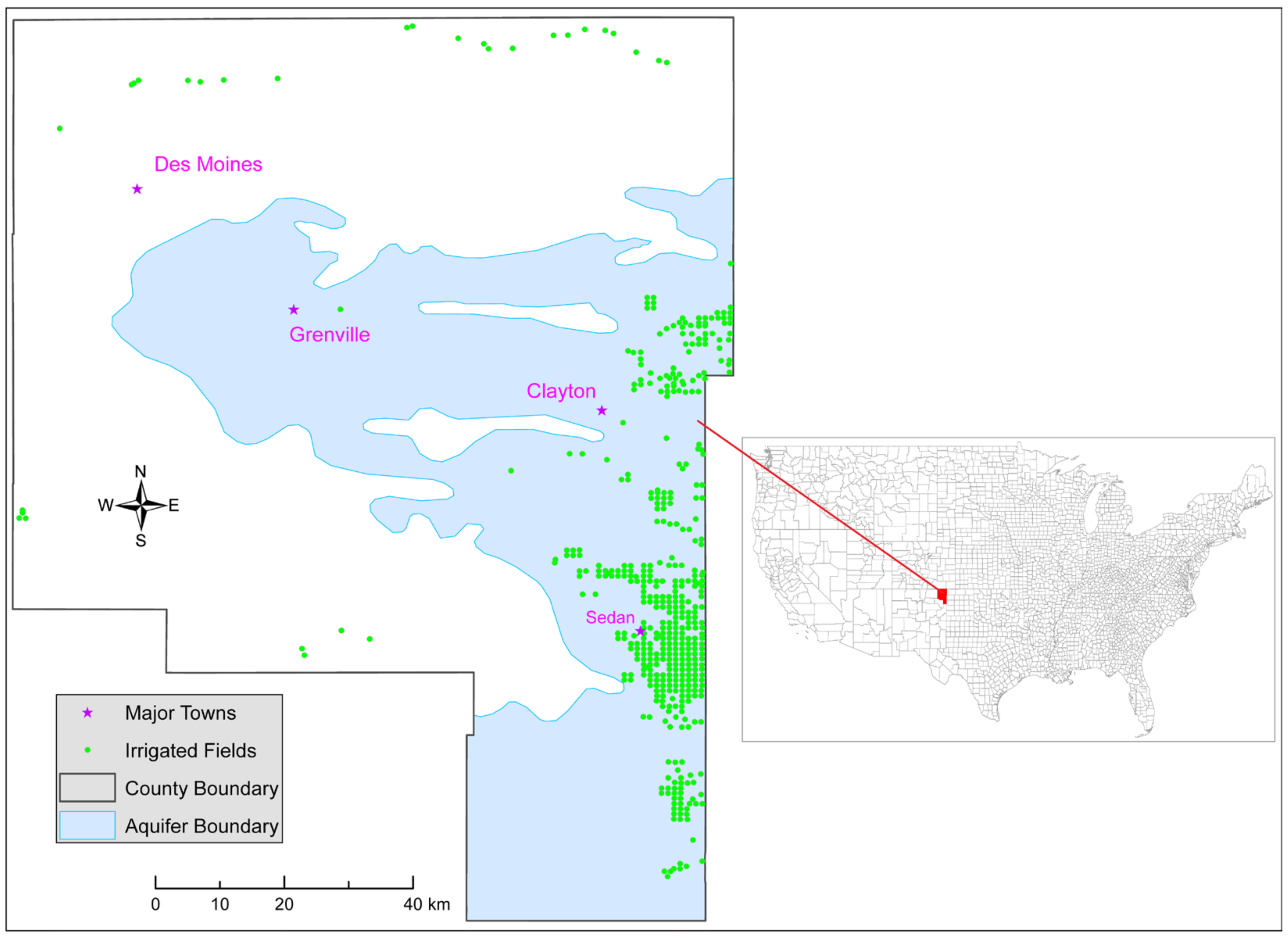
  • Field Identification: Based on 2022 Google Maps imagery data, I identified 472 unique irrigated crop fields in Union County and the center of their X–Y geographic coordinates. For the few unclear ones, I validated them with local stakeholders. Figure A2 in Appendix A illustrates the circular irrigated fields in the central–eastern and southeastern parts of the county where most of the irrigation happens.
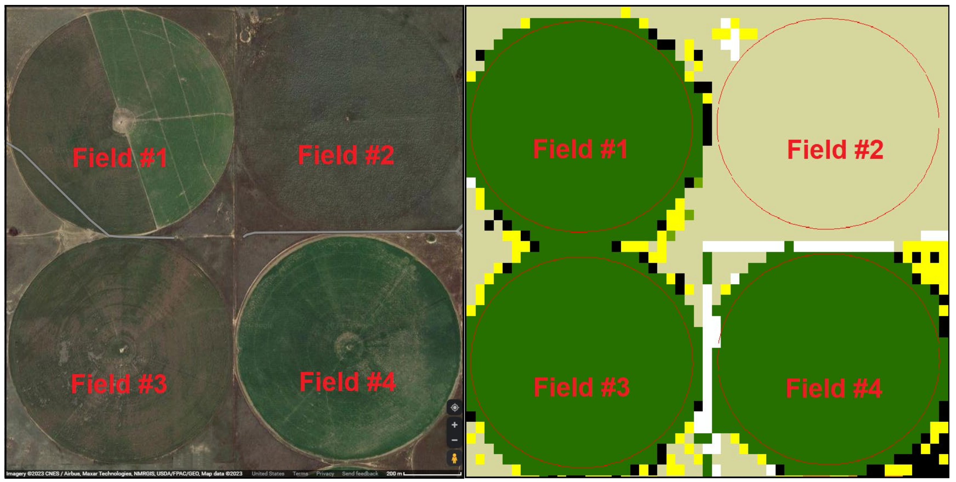
  • Radius Determination: I measured the radius of each circular field using the ‘Measure Distance’ tool in Google Maps. The standard circular irrigated field has a radius of around 400 m (see Figure 2). The radius of all circular irrigated fields ranges from 120 m to 830 m, and over 70% have a standard 400 m radius.
  • Buffering: To compute the proportions of each crop and grassland inside a field, I buffered the field center by 90% of its radius and then counted the shares of different pixels within the buffered circle (e.g., if the field radius is 400 m, then the buffered area has a radius of 360 m). This is to reduce potential measurement errors near field boundaries.
I obtained groundwater depth (land surface to the water table) data from the national groundwater levels monitoring database (https://waterdata.usgs.gov/nm/nwis/gw (accessed on 19 March 2023)) maintained by the USGS. This study uses groundwater level data from 2007 to 2018 to generate expected groundwater levels for the years 2008–2019 (study period) with an AR (autoregressive) model of degree 1 (AR (1)). The model statistically regresses the current groundwater level value linearly on its previous value and a stochastic error term. The estimated linear regression model can then be used to take a given groundwater level observation to predict the next period’s groundwater level. Its key model assumption is that the groundwater level time series is stationary over time, which usually holds for slow-changing measures such as groundwater levels. It is convenient to use for simple prediction needs such as here, and it captures farmers’ short-memory decision-making behavior well [18]. During the study period, 607 groundwater level observations were recorded from 111 wells (see Figure A3 in Appendix A). It is clear that not every irrigated field had its well’s water level recorded. Hence, I used two spatial interpolation methods to estimate the annual groundwater level for each of the 472 unique crop fields: simple average and inverse distance weighted average. The range of the spatial interpolation is 16 km (roughly 10 US miles). That is, for any given year, all well water level observations within 16 km of a crop field are used to approximate the groundwater level of that field if there is no direct water level observation from the given crop field.
Additionally, the planned empirical analysis includes local precipitation and temperature as control variables. Following the convention in the literature, I used the average monthly mean temperature in the growing season (April–October in the study region) and total growing season precipitation as control variables. Given that the monsoon season brings most of the annual precipitation and that it matches the growing season in the region, the growing season’s climatic conditions are the most relevant to control. The raw monthly climate data series used to compute the two climatic variables comes from the PRISM data developed by Oregon State University. Lastly, all of the GIS shapefiles used to define jurisdictional and aquifer boundaries, such as those in Figure 1, come from the US Census and the US Geological Survey. Table A1 in Appendix A summarizes the source, collection time, format, and other relevant information of all data used in this study.

2.2. The Empirical Methodology

Switching back to grassland as a result of exogenous impacts in a given area can be modeled from either a probabilistic perspective or a proportional perspective. Both perspectives share the same mathematical characteristic in that the dependent variable is measured between 0 and 1 (or equivalently, between 0% and 100%). Such a bounded dependent variable cannot be directly part of a linear regression model. In this study, I follow the standard approach of transforming it into a log odds model that is rooted in the classic logistic regression model [18,19]. This study hypothesizes that an expected groundwater level change affects crop choice and the probability of switching from cropland back to grassland. For a given field i in year t , let us denote the proportion of grassland as P i t , which essentially approximates the probability of being grassland using the empirically observed proportion of grassland. The statistical odds (ratio) of switching back to grassland are then defined as P i t / 1 P i t . With the logarithm transformation of the odds ratio being the dependent variable, we can now use a (transformed) linear regression model to examine the impact of an expected groundwater level change on the probability of switching back to grassland:
l o g P i t 1 P i t = β 1 G W L i t + β 2 P P T i t 1 + β 3 T m e a n i t 1 + δ i + μ t + ε i t
In Equation (1), G W L i t is the expected groundwater level at field i in year t , as discussed in Section 2.1. Coefficient β 1 is thus the key associated parameter to be estimated. P P T i t and T m e a n i t are control variables for climatic variabilities. As the corresponding subscripts in Equation (1) suggest, here we choose to use one-year-lagged growing season total precipitation and average monthly mean temperature measures. First and foremost, the cropland allocation decision is made early in the spring before the monsoon season starts. Hence, farmers cannot possibly factor the to-be-observed current-year precipitation and temperature conditions into production decisions. Second, the one-year-lagged climatic measures provide simple and realistic proxies (i.e., heuristics) for precipitation and temperature conditions in the coming growing season.
The linear regression model proposed in Equation (1) is often termed a two-way (panel data) fixed-effects model. Because the model simultaneously controls for two different fixed effects: spatial and temporal. In this case, δ i represents time-invariant spatial fixed effects to implicitly control any spatial heterogeneities unique to each crop field, and μ t represents time-varying temporal fixed effects to absorb any region-wide time trends affecting cropland use decisions, such as market prices and policy changes. The error term ε i t helps capture any random shocks to cropland allocation decisions. It is worth noting that the proposed framework in Equation (1) only considers crop choices among major commercial crops observed in the region and the possible switch between cropland and grassland. It does not cover the possibility of converting agricultural land to other land uses such as residential development.
Based on crop statistics from the CDL data during the study period and the recent New Mexico Agricultural Statistics Bulletins [20], the log odds model is estimated for three major commercial crops (corn (for silage, mainly), winter wheat, and sorghum) and grassland. The focus of the analysis is on grassland, while results with the three major commercial crops serve as comparisons. Table 1 summarizes all variables relevant to the regression analyses of all four choices. Please note that the actual model estimation can only use 441 crop fields out of 472. The other 31 fields are automatically excluded due to a lack of variation during the study period (e.g., due to monocropping).

2.3. Marginal Impact

Due to the log odds transformation of the dependent variable in Equation (1), the parameter estimates β 1 to β 3 cannot be interpreted as marginal effects directly. Taking the key variable of interest G W L i t as an example, β 1 is not directly the marginal impact of groundwater level change on the proportion of grassland, namely β 1 P i t / G W L i t . To get the true marginal effect of G W L i t , we need another transformation. Let β ^ , δ ^ , and μ ^ denote the estimated coefficients and fixed effects, thus allowing the predicted P i t value to be obtained by the following:
P ^ i t = exp β ^ 1 G W L i t + β ^ 2 P P T i t 1 + β ^ 3 T m e a n i t 1 + δ ^ i + μ ^ t 1 + exp β ^ 1 G W L i t + β ^ 2 P P T i t 1 + β ^ 3 T m e a n i t 1 + δ ^ i + μ ^ t
Given Equation (2), the true individual marginal effect can be computed as:
P ^ i t G W L i t = β ^ 1 exp β ^ 1 G W L i t + β ^ 2 P P T i t 1 + β ^ 3 T m e a n i t 1 + δ ^ i + μ ^ t 1 + exp β ^ 1 G W L i t + β ^ 2 P P T i t 1 + β ^ 3 T m e a n i t 1 + δ ^ i + μ ^ t 2
Empirical computation of the average marginal effect (AME) of G W L i t for the study area (the entire sample) and the associated estimation of its standard error will be discussed in the following Section 3.

3. Results

3.1. Regression Estimation Results

As discussed above in Section 2, the empirical estimation takes two steps. The first step estimates the log odds model in Equation (1) to obtain coefficient and fixed-effect estimates β ^ (and their variance–covariance matrix), δ ^ , and μ ^ . The second step computes the true marginal effects and derives their standard errors using the delta method based on Equation (3). To implement the estimation steps, some data transformations are necessary. The raw data sample contains observations with dependent variable values of 0 (e.g., no grassland pixels) or 1 (e.g., all grassland pixels). In such cases, the log odds transformation does not work in Equation (1). To address this computational issue, I re-coded observations. The values were set from 0 to 0.000001 and from 1 to 0.999999. The transformations allow the estimation procedure to proceed without modifying the data in any significant way. Table 2 presents the estimation results for three major commercial crops and grassland. As mentioned before, two different specifications of groundwater level are explored here: simple average (specification 1) and inverse distance weighted average (specification 2).
Although the coefficient estimates in Table 2 cannot be directly interpreted as the marginal effects, several qualitative observations related to groundwater level decline can be established. It is worth emphasizing again that groundwater level is measured as the distance from land surface to water table. That is, groundwater level decline leads to an increase in GWL as measured in Equation (1). Looking at Table 2, the positive coefficient estimates for GWL suggest that groundwater level decline increases the odds of growing corn (for silage) and sorghum and switching back to grassland. The results for corn and sorghum are intuitive. Corn for silage does not have to follow a regular irrigation schedule as it is not planted for grain yield. Hence, it can be considered “drought-resistant.” Sorghum is a commonly adopted drought-resistant grain crop in the High Plains. Switching to grassland essentially cuts irrigation water demand to zero. It is expected to be the most effective adaptation strategy to multi-year persistent droughts. It makes sense to have more land switching back to grassland to conserve water in anticipation of groundwater level decline. Second, the negative coefficient estimates for GWL suggest that groundwater level decline reduces the odds of growing wheat (mainly winter wheat in the study region). There are two potential explanations. The first explanation is the long growing season of winter wheat, which is around eight months. This increases the crop’s vulnerability to droughts. The second explanation is the crop irrigation water demand. Winter wheat for grain has an irrigation water demand of around 20 inches, which is close to sorghum. Nevertheless, sorghum is a more drought-resilient option assuming a similar expected economic return (output revenue minus input costs) between the two crops. This explains the preference for sorghum over winter wheat in anticipation of groundwater level decline.
By comparing results across four different models (columns in Table 2), one noticeable pattern is that the three commercial crops are more responsive to groundwater level changes in terms of coefficient estimate magnitudes. This makes sense because the choice of field crop is a reversible land allocation choice, while switching to grassland tends to be irreversible, at least in the near-to-medium term. Another noticeable pattern from the comparison is the significantly higher goodness of fit (R2, within) of the grassland model (last column in Table 2). This suggests that groundwater level coupled with growing season precipitation and temperature better explain the odds of switching to grassland compared to other crops. One potential explanation is that commercial crop planting decisions are more sensitive to market and policy factors. Additionally, the temporal fixed effects in the model may not absorb them entirely.
One thing to note is that the precipitation and temperature measures here serve only as control variables. They are more relevant factors in rain-fed cropping regions [1]. Hence, I refrain from interpreting their coefficient estimates to stay focused on the given research question concerning grassland in this study. Another thing to note is the implicit assumption embedded in the analysis that farmers usually explore other options (such as drought-tolerant crops, land idling, and crop rotation) before considering switching back to grassland permanently. This is consistent with my communications with local stakeholders.

3.2. Marginal Impacts of Groundwater Level Decline

As demonstrated in Equation (3), the true marginal effects require a transformation derived from the estimates of coefficients and fixed effects in Table 2. For simplicity and ease of interpretation, I compute the average marginal effect (AME). The first step is to compute the marginal effect for each observation following Equation (3). Subsequently taking the average of all individual marginal effects obtains the AME:
A M E = P ^ G W L = 1 N T t = 1 T i = 1 N P ^ i t G W L i t
where N is the total number of crop fields and T is the total number of years studied. Such a way of computing the marginal impact of groundwater level decline allows us to incorporate each of the individual spatial and temporal fixed effects into consideration, which are important for field-level analyses such as those in the current study.
Table 3 presents the computed marginal effects based on Equation (4) and the corresponding standard errors approximated using the delta method. Overall, the three commercial crops are more responsive to groundwater level decline based on the marginal effect magnitudes, which is consistent with the estimates in Table 2. However, the estimates are not statistically significant. This is likely due to the poor overall fit of these three models, as discussed in the previous section. The potential correlation between GWL and growing season precipitation and temperature is another possible contributor to the low precision. The marginal effect of groundwater level decline on grassland, although at a smaller magnitude, is statistically significant (5% for specification (1) and 10% for specification (2)). Taking specification (1) as an example, a marginal effect estimate of 0.0494 means that for every foot of groundwater level decline, the likelihood of switching back to grassland increases by roughly 0.05%. In other words, for a one-standard-deviation decline in groundwater level (36.95 feet, see Table 1), the likelihood of switching back to grassland increases by 1.85%. Although this is not a large impact in terms of magnitude, it is a permanent cropland use change, as emphasized before. Its long-term socio-economic and policy implications can be significant. The following Section 4 will explore the economic and policy implications of the results.

4. Policy Discussion

The research question of this study and the following empirical findings directly concern the economic and social values of grassland. In the agricultural sector, grassland often serves as pasture to generate private economic value. In other cases, grassland generates environmental conservation values that benefit the broader society. For example, grassland is commonly considered one of the best natural carbon sinks [21]. The current study has shown that, with an anticipated decline in groundwater level in the Ogallala Aquifer, local farmers are voluntarily (or are forced to) switching back to grassland to adapt to agricultural droughts. With the changing monsoon dynamics in the southwest US [22], drought conditions are expected to be more frequent and persistent. Switching to more drought-tolerant crops or pasture grassland seems to be a natural strategy for adaptation. A critical question to ask here is whether less crop production and more pasture can generate enough economic value to sustain the local agribusiness and economy. There are two aspects to this question. The first aspect concerns the direct economic value of additional pasture, which is private to landowners or operators. This economic value should consist of at least two components: (1) the profit from livestock production on natural grassland, which usually generates a premium on the market; and (2) the complementary value from the grassland ecosystem that spills over to crop production, such as water catchments (see [23] for a review), which can be defined as an equitable economic value to the local agricultural community. The other aspect relates to the broader social value that can catalyze economic value added beyond traditional agricultural production. For example, expanded grassland areas can create opportunities for wildlife habitats and recreational landscapes that offer further opportunities for agritourism. The empirical estimates from this study can provide necessary parameters for the accounting of these economic values from added pasture grassland.
Another important policy implication of switching back to grassland is the conservation values that concern local land (soil) and water resources. In the study region and the broader Southern High Plains, soil and groundwater conservation are as equally important as they are interconnected. The dust storms that occurred in the region during the 1930s were an example of soil conservation failure (and to some extent a water conservation failure). Nowadays, because of the widespread groundwater irrigation practice in the region, it has become even more critical to coordinate soil and water conservation. Soil conservation in the region typically entails reducing soil erosion and improving soil health. Permanent grassland can help achieve both goals [24]. Water conservation tends to be more complicated in the region due to the fact that the groundwater aquifer is shared across the state boundary between New Mexico and Texas. Additionally, crop agriculture in the region withdraws over 90% of its irrigation water from groundwater aquifers despite the fact that groundwater wells are relatively well regulated in New Mexico [25]. Given that groundwater is the dominant water resource in the region, water conservation entails recharge management, pumping management, and transboundary coordination, among other things. Even though water conservation is more challenging in the region, it complements land and soil conservation. As shown in this study, groundwater dynamics affect cropland allocation decisions. On the other hand, it is common knowledge that land (soil) conservation facilitates surface infiltration processes and thus affects groundwater aquifer recharge [26]. Therefore, soil conservation and groundwater conservation can become part of an integrated two-fold conservation strategy. The empirical results from this study help us to understand at least one of the mechanisms for integration.
No matter if it is the added value from pasture-based livestock production or the broader social value from improved soil and water conservation, the bottom line is that these conservation efforts should be able to help strengthen and sustain rural economic livelihoods. Otherwise, switching back to grassland may find little practical policy significance. Many drought-stressed agricultural communities face not only environmental and resource challenges, but also demographic stagnation. Brain drain and inadequate agricultural workforce pipelines have been prime challenges in many rural communities [27]. Any policy that aims to address environmental and resource problems but which fails to simultaneously meet local economic development needs is unlikely to work or last. To successfully integrate the two (i.e., building environmental and natural resource stewardship and promoting local economic development), it is critical to estimate key parameters and metrics precisely. This is what the current study intends to contribute toward. By quantifying the impacts of groundwater level decline on field-level cropland allocation decisions, we can help establish a measurable link between the hydrological sub-system and the surface land vegetation sub-system for an integrated ecosystem. It can then be further incorporated into tasks such as resource use efficiency assessment, sustainability policy design, etc.

5. Conclusions

Groundwater resources play an indispensable role in economic and human development in arid/semi-arid regions around the world. When it comes to agricultural production, groundwater often becomes one of the most critical determinants of yield and profitability. This is particularly true for the High Plains region in the US. In recent decades, growing concern over irrigated crop production relates to the increasing variability in agricultural droughts and groundwater depletion. In the context of changing monsoon dynamics in the Southwest and growing drought vulnerability faced by farmers, this study aims to help understand how groundwater level decline affects the likelihood of cropland switching back to grassland as a way to adapt. Taking Union County of New Mexico as a case study, this study finds that cropland has been slowly but permanently switching back to grassland as the groundwater level in the Ogallala Aquifer has continued to decline.
The implication of the findings is long term. In the near term, irrigated commercial crops such as corn, winter wheat, and sorghum will still dominate the region’s cultivated landscape. However, as the groundwater level continues to decline, the pace of switching back to dryland farming and grassland will accelerate. Meanwhile, such cropland use changes likely go from being voluntary to being forced as choices become limited. The long-term environmental and socio-economic consequences of such a shift are unknown. What is clear is that, if this process is not guided and managed properly, there will be catastrophic consequences similar to or worse than those of the Dust Bowl on the High Plains during the 1930s. Therefore, understanding this transition process and its potential impacts at each stage is essential. It is not only for the benefit of designing better groundwater conservation policies, but also for educating the next generation of the agricultural workforce. Lastly, it is worth mentioning that this study also showcases how increasingly available remote sensing data can be integrated with traditional statistical data collected by government agencies and other organizations to answer urgent rural economic development and environmental sustainability questions.
Future research can build upon this study to expand in a few directions. First, new data analytics methods can help develop better quantification of groundwater scenarios under a changing climate. For example, machine learning models can help resolve the intermittent sampling frequency issue associated with groundwater data monitoring [28]. Second, advanced remote sensing technologies may be integrated with data analytics to develop alternative measures of groundwater level, which can help improve the spatial solution of the data (see [29] for an early example). The OpenET data platform (https://openetdata.org/ (accessed on 19 March 2023)) is an exemplary application in this direction. It integrates publicly available data to provide satellite-based information on evapotranspiration, which can provide alternative and better ways to understand groundwater dynamics. Third, farmers’ adaptation choice sets could expand as new technologies become economically feasible and more integrated into the existing production system. This study assumes that farmers are limited to a traditional choice set of field crops and grassland. In the future, more integrated production systems such as solar gardens (e.g., a crop or produce farm under a solar farm) and greenhouses powered with renewable energy may become widely feasible. These newer choices could have new impacts on groundwater resources, positive or negative, which points to a fruitful direction for future research.

Funding

This research was jointly funded by the USDA National Institute of Food and Agriculture (NIFA) under award 2022-67020-36265 and the New Mexico Water Resources Research Institute (NM WRRI) under award Q02304 (the USGS-104B Faculty Water Research Grant Program). The APC was funded by NM WRRI award Q02304.

Data Availability Statement

The CDL land cover data (raster files) are downloadable at https://nassgeodata.gmu.edu/CropScape/ (accessed on 19 March 2023). The climate data (raster files) are downloadable at https://prism.oregonstate.edu/ (accessed on 19 March 2023). The raw records on groundwater levels (spreadsheet files) are downloadable at https://waterdata.usgs.gov/nm/nwis/gw (accessed on 19 March 2023). All other data are available from the author upon request.

Acknowledgments

The author would like to thank Talisha Valdez of the Union County (New Mexico) Extension Office and Ben Creighton of the USDA NRCS Union County (New Mexico) Office for their help in motivating this research. All errors belong to the author.

Conflicts of Interest

The authors declare no conflict of interest.

Appendix A

Figure A1. The relative geographic location of Union County, New Mexico, in the broader region. Note: the local landscape features mainly natural grassland and (mostly irrigated) crop agriculture. Data source: US Census.
Remotesensing 15 01698 g0a1
Figure A2. Identified circular irrigated crop field boundaries overlapped with Crop Data Layer data in the central–eastern and southeastern parts of Union County, New Mexico. Note: light green in the background indicates grassland and other colors indicate different crop covers. Data source: NASS, USDA; Google Maps.
Remotesensing 15 01698 g0a2
Figure A3. The USGS monitored wells that recorded groundwater level data during the study period (2007–2019). Note: A total of 111 well locations are illustrated on the map. There is only one weather station in the county (Clayton Municipal Airpark (KCAO); Lat: 36.45°N; Lon: 103.15°W), located near Clayton. Data sources: US Geological Survey; US Census.
Remotesensing 15 01698 g0a3
Table A1. Supplemental information on datasets used in this study.
DataSourceCollection TimeFormat
Crop Data LayerNASS, USDAAnnualRaster
Groundwater levelsUS Geological SurveyAnnualCSV
PRISMOregon State UniversityAnnualRaster
Field location and sizeGoogle Maps2022CSV
GIS MapsUS Census; US Geological Survey2020Shapefiles
Note: for annually available datasets, data from the years 2007 to 2019 have been retrieved.

References

  1. Ortiz-Bobea, A.; Wang, H.; Carrillo, C.M.; Ault, T.R. Unpacking the climatic drivers of US agricultural yields. Environ. Res. Lett. 2019, 14, 064003. [Google Scholar] [CrossRef]
  2. McKenna, O.P.; Sala, O.E. Groundwater recharge in desert playas: Current rates and future effects of climate change. Environ. Res. Lett. 2017, 13, 014025. [Google Scholar] [CrossRef]
  3. Scanlon, B.R.; Faunt, C.C.; Longuevergne, L.; Reedy, R.C.; Alley, W.M.; McGuire, V.L.; McMahon, P.B. Groundwater depletion and sustainability of irrigation in the US High Plains and Central Valley. Proc. Natl. Acad. Sci. USA 2012, 109, 9320–9325. [Google Scholar] [CrossRef] [Green Version]
  4. Roy, P.; Pal, S.C.; Chakrabortty, R.; Chowdhuri, I.; Saha, A.; Shit, M. Climate change and groundwater overdraft impacts on agricultural drought in India: Vulnerability assessment, food security measures and policy recommendation. Sci. Total Environ. 2022, 849, 157850. [Google Scholar] [CrossRef]
  5. Sophocleous, M. Review: Groundwater management practices, challenges, and innovations in the High Plains aquifer, USA—Lessons and recommended actions. Hydrogeol. J. 2010, 18, 559–575. [Google Scholar] [CrossRef]
  6. Theesfeld, I. Institutional challenges for national groundwater governance: Policies and issues. Groundwater 2010, 48, 131–142. [Google Scholar] [CrossRef] [PubMed] [Green Version]
  7. Blomquist, W.; Schlager, E.; Heikkila, T. Common Waters, Diverging Streams: Linking Institutions and Water Management in Arizona, California, and Colorado; Routledge: New York, NY, USA, 2010; pp. 1–19. [Google Scholar]
  8. Gonçalves, I.Z.; Mekonnen, M.M.; Neale, C.M.; Campos, I.; Neale, M.R. Temporal and spatial variations of irrigation water use for commercial corn fields in Central Nebraska. Agric. Water Manag. 2020, 228, 105924. [Google Scholar] [CrossRef]
  9. Gilbert, G.; McLeman, R. Household access to capital and its effects on drought adaptation and migration: A case study of rural Alberta in the 1930s. Popul. Environ. 2010, 32, 3–26. [Google Scholar] [CrossRef]
  10. Staggenborg, S.A.; Dhuyvetter, K.C.; Gordon, W.B. Grain sorghum and corn comparisons: Yield, economic, and environmental responses. Agron. J 2008, 100, 1600–1604. [Google Scholar] [CrossRef] [Green Version]
  11. Arellano-Gonzalez, J.; Moore, F.C. Intertemporal arbitrage of water and long-term agricultural investments: Drought, groundwater banking, and perennial cropping decisions in California. Am. J. Agric. Econ. 2020, 102, 1368–1382. [Google Scholar] [CrossRef]
  12. Gebremichael, M.; Krishnamurthy, P.K.; Ghebremichael, L.T.; Alam, S. What drives crop land use change during multi-year droughts in California’s Central Valley? Prices or concern for water? Remote Sens. 2021, 13, 650. [Google Scholar] [CrossRef]
  13. Deines, J.M.; Schipanski, M.E.; Golden, B.; Zipper, S.C.; Nozari, S.; Rottler, C.; Guerrero, B.; Sharda, V. Transitions from irrigated to dryland agriculture in the Ogallala Aquifer: Land use suitability and regional economic impacts. Agric. Water Manag. 2020, 233, 106061. [Google Scholar] [CrossRef]
  14. Cotterman, K.A.; Kendall, A.D.; Basso, B.; Hyndman, D.W. Groundwater depletion and climate change: Future prospects of crop production in the Central High Plains Aquifer. Clim. Chang. 2018, 146, 187–200. [Google Scholar] [CrossRef]
  15. Phillips, S.T. Lessons from the dust bowl: Dryland agriculture and soil erosion in the United States and South Africa, 1900–1950. Environ. Hist. 1999, 4, 245–266. [Google Scholar] [CrossRef]
  16. Foster, T.; Brozović, N.; Butler, A.P. Effects of initial aquifer conditions on economic benefits from groundwater conservation. Water Resour. Res. 2017, 53, 744–762. [Google Scholar] [CrossRef] [Green Version]
  17. Tran, D.Q.; Kovacs, K.; Wallander, S. Water conservation with managed aquifer recharge under increased drought risk. Environ. Manag. 2020, 66, 664–682. [Google Scholar] [CrossRef]
  18. Wang, H.; Ortiz-Bobea, A. Market-driven corn monocropping in the US Midwest. Agric. Resour. Econ. Rev. 2019, 48, 274–296. [Google Scholar] [CrossRef] [Green Version]
  19. Papke, L.E.; Wooldridge, J.M. Econometric methods for fractional response variables with an application to 401 (k) plan participation rates. J Appl. Econom. 1996, 11, 619–632. [Google Scholar] [CrossRef]
  20. NASS; USDA. New Mexico Annual Statistics Bulletins. Available online: https://www.nass.usda.gov/Statistics_by_State/New_Mexico/Publications/Annual_Statistical_Bulletin/index.php (accessed on 1 December 2022).
  21. Dass, P.; Houlton, B.Z.; Wang, Y.; Warlind, D. Grasslands may be more reliable carbon sinks than forests in California. Environ. Res. Lett. 2018, 13, 074027. [Google Scholar] [CrossRef]
  22. Pascale, S.; Boos, W.R.; Bordoni, S.; Delworth, T.L.; Kapnick, S.B.; Murakami, H.; Vecchi, G.; Zhang, W. Weakening of the North American monsoon with global warming. Nat. Clim. Chang. 2017, 7, 806–812. [Google Scholar] [CrossRef]
  23. Boval, M.; Dixon, R.M. The importance of grasslands for animal production and other functions: A review on management and methodological progress in the tropics. Animal 2012, 6, 748–762. [Google Scholar] [CrossRef] [PubMed] [Green Version]
  24. De, M.; Riopel, J.A.; Cihacek, L.J.; Lawrinenko, M.; Baldwin-Kordick, R.; Hall, S.J.; McDaniel, M.D. Soil health recovery after grassland reestablishment on cropland: The effects of time and topographic position. Soil Sci. Soc. Am. J. 2020, 84, 568–586. [Google Scholar] [CrossRef]
  25. Mrad, A.; Katul, G.G.; Levia, D.F.; Guswa, A.J.; Boyer, E.W.; Bruen, M.; Carlyle-Moses, D.E.; Coyte, R.; Creed, I.F.; Van De Giesen, N.; et al. Peak grain forecasts for the US High Plains amid withering waters. Proc. Natl. Acad. Sci. USA 2020, 117, 26145–26150. [Google Scholar] [CrossRef]
  26. Ilstedt, U.; Bargués Tobella, A.; Bazié, H.R.; Bayala, J.; Verbeeten, E.; Nyberg, G.; Sanou, J.; Benegas, L.; Murdiyarso, D.; Laudon, H.; et al. Intermediate tree cover can maximize groundwater recharge in the seasonally dry tropics. Sci. Rep. 2016, 6, 21930. [Google Scholar] [CrossRef] [Green Version]
  27. Carr, J.P.; Kefalas, J.M. The Rural Brain Drain. The Chronicle of Higher Education, 21 September 2009. Available online: https://chronicle.com/article/the-rural-brain-drain/ (accessed on 10 January 2023).
  28. Xiong, J.; Guo, S.; Kinouchi, T. Leveraging machine learning methods to quantify 50 years of dwindling groundwater in India. Sci. Total Environ. 2022, 835, 155474. [Google Scholar] [CrossRef] [PubMed]
  29. Anderson, R.G.; Lo, M.H.; Famiglietti, J.S. Assessing surface water consumption using remotely-sensed groundwater, evapotranspiration, and precipitation. Geophys. Res. Lett. 2012, 39, L16401. [Google Scholar] [CrossRef] [Green Version]
Figure 1. The High Plains (Ogallala) Aquifer and irrigated crop fields in Union County, New Mexico. Data Source: US Geological Survey, US Census, and Google Maps. Note: (1) A total of 472 circular irrigated fields are illustrated on the map. (2) The aquifer map was published in 2010 by the US Geological Survey (see https://pubs.usgs.gov/ds/543/ (accessed on 19 March 2023)).
Remotesensing 15 01698 g001
Figure 2. A standard 400 m radius irrigated field (field #2) in its transition into grassland (left panel) compared to the remotely sensed Crop Data Layer (right panel, 2019 data) of the same location. Data Source: NASS, USDA; Google Maps. Note: The remote sensing data in the right panel indicate that corn (in dark green) was grown in fields #1, #3, and #4 in 2019. Later, in 2021 (corresponding to the time of the left panel Google Maps imagery), field #3 was in idle status and fields #1 and #4 still had corn.
Remotesensing 15 01698 g002
Table 1. Summary statistics and variable definitions.
VariableDefinitionMeanStd. Dev.
Freq_cornProportion of corn pixels, in [0, 1]0.290.42
Freq_wheatProportion of wheat pixels, in [0, 1]0.500.45
Freq_sorghumProportion of sorghum pixels, in [0, 1]0.040.17
Freq_grassProportion of grassland/pasture pixels, in [0, 1]0.130.30
PPT1-year-lagged growing season total precipitation, mm390.18129.90
T_mean1-year-lagged growing season mean monthly temperature, °C18.990.62
GWL_meanSimple average local groundwater level, feet210.1936.95
GWL_inv_distInverse distance weighted local groundwater level, feet216.1140.48
Lodds_cornLog odds of corn proportion, unit free−5.2410.04
Lodds_wheatLog odds of wheat proportion, unit free−0.0110.14
Lodds_sorghumLog odds of sorghum proportion, unit free−11.295.21
Lodds_grassLog odds of grassland/pasture proportion, unit free−9.096.87
# of obsNumber of observations in the estimation sample5292
# of fieldsNumber of irrigated fields in the estimation sample441
YearsYears covered in the study period12 (2008–2019)
Note: 1. As 441 × 12 = 5292, this suggests that the estimation sample is a balanced panel dataset. 2. Wheat in the study region (Union County, New Mexico) is mostly winter wheat. 3. The growing season is the seven-month period from April to October in the study region. 4. For conversion, 1 US foot = 30.48 cm.
Table 2. Estimation results from the (panel data) two-way fixed-effects model.
Cropland Log Odds Model
SpecificationVariablesCornWheatSorghumGrassland
(1)P—lagged (mm)−0.0026
(0.0032)
0.0093 ***
(0.0032)
−0.0087 ***
(0.0019)
−0.0072 ***
(0.0016)
T—lagged (C)−4.5465 **
(1.8966)
3.9575 **
(1.9249)
−0.6185
(1.1256)
−4.6738 ***
(0.9615)
GWL (foot):
simple average
0.0499 ***
(0.0141)
−0.0680 ***
(0.0143)
0.0428 ***
(0.0083)
0.0316 ***
(0.0071)
R2—within0.05800.04590.08190.1617
# of observations5292529252925292
Fixed EffectsField + Year
(2)P—lagged (mm)−0.0024
(0.0032)
0.0091 ***
(0.0032)
−0.0086 ***
(0.0019)
−0.0071 ***
(0.0016)
T—lagged (C)−4.1878 **
(1.8859)
3.5266 *
(1.9139)
−0.2741
(1.1198)
−4.2991 ***
(0.9572)
GWL (foot):
inverse distance weighted
0.0467 ***
(0.0142)
−0.0679 ***
(0.0144)
0.0375 ***
(0.0085)
0.0189 ***
(0.0072)
R2—within0.05760.04580.08060.1595
# of observations5292529252925292
Fixed EffectsField + Year
Note: (1) Asterisks (*, **, ***) indicate statistical significance at levels of 10%, 5% and 1%, respectively, unless otherwise noted. (2) Standard errors are reported in the parentheses. (3) The growing season is the seven months from April to October in the study region. (4) For conversion, 1 US foot = 30.48 cm.
Table 3. Estimated average marginal effects of groundwater level decline.
Cropland Proportion Model
SpecificationVariablesCornWheatSorghumGrassland
(1)GWL—simple average
(unit: % per foot)
0.1509
(0.6961)
−0.3983
(0.4714)
0.0070
(0.0761)
0.0494 **
(0.0237)
Fixed EffectsField + Year
(2)GWL—inverse distance weighted
(unit: % per foot)
0.1412
(0.6885)
−0.4003
(0.4927)
0.0060
(0.0654)
0.0295 *
(0.0172)
Fixed EffectsField + Year
Note: (1) Asterisks (*, **) indicate statistical significance at levels of 10% and 5%, respectively, unless otherwise noted. (2) Standard errors are reported in the parentheses. (3) For conversion, 1 US foot = 30.48 cm.
Disclaimer/Publisher’s Note: The statements, opinions and data contained in all publications are solely those of the individual author(s) and contributor(s) and not of MDPI and/or the editor(s). MDPI and/or the editor(s) disclaim responsibility for any injury to people or property resulting from any ideas, methods, instructions or products referred to in the content.

