A Modified NLCS Algorithm for High-Speed Bistatic Forward-Looking SAR Focusing with Spaceborne Illuminator

Abstract

The coupling and spatial variation of range and azimuth parameters is the biggest challenge for bistatic forward-looking SAR (BFSAR) imaging. In contrast with the monostatic SAR and translational invariant bistatic SAR (TI-BSAR), the range cell migration (RCM), and Doppler parameters of high-speed bistatic forward-looking SAR (HS-BFSAR) have two-dimensional spatial variation characteristics, which makes it difficult to obtain SAR images with satisfactory global focusing. Firstly, based on the configuration of the spaceborne illuminator and high-speed forward-looking receiving platform, the accurate range-Doppler domain expression of the echo signal is derived in this paper. Secondly, using this analytical expression, a range nonlinear chirp scaling (NLCS) is proposed to equalize the RCM and equivalent range frequency modulation (FM) rate so that they can be uniformly processed in the two-dimensional frequency domain. Next, in the azimuth processing, the proposed method decomposes the Doppler contribution of the transmitter and receiver, respectively. Then, an azimuth NLCS is used to eliminate the spatial variation of the azimuth FM rate. Finally, a range-dependent azimuth filter is constructed to achieve azimuth compression. Simulation results validate the efficiency and effectiveness of the proposed algorithm.

1. Introduction

For decades, synthetic aperture radar (SAR) has been widely used in civil remote sensing and military fields because of its advantages which can provide high-resolution images of the observation area without being affected by weather conditions, regardless of whether it is day or night [1,2,3,4]. Moreover, the electromagnetic waves emitted by the SAR also have a certain penetrability, which can find some sheltered underground structures [5]. For instance, scientists discovered the ancient river channel of the Nile in the Sahara Desert with the help of SAR satellites [6]. However, the traditional monostatic SAR cannot obtain two-dimensional resolution due to the overlap between its range gradient and Doppler gradient in the case of forward-looking reception [7]. This limits the application of SAR technology in trajectory planning, terminal guidance, autonomous landing, and other fields. Fortunately, bistatic SAR (BiSAR) has been proven to solve this problem [8]. By placing the transmitter and receiver on two separate platforms, BiSAR can be designed to make the range gradient and Doppler gradient of the forward-looking region no longer coincide, so as to obtain the two-dimensional forward-looking resolving ability [9]. Compared with monostatic SAR, the BiSAR receiver has flexible configuration and eminent concealment, as well as achieves more information in feature extraction and classification. Due to these advantages, BiSAR has attracted increasing research interest in the past decade [10,11,12,13,14].

The transmitter and receiver in BiSAR have independent trajectories, therefore the geometric configuration has ample flexibility. Bistatic SAR operating in forward-looking imaging configuration is called bistatic forward-looking SAR (BFSAR), which has attracted much attention because of its forward-looking two-dimensional resolution. In reference [15], BFSAR is categorized into three types: translation invariant (TI), translation variation (TV), and stationary transmitter cases. In TI mode, the transmitter and receiver platforms have the same velocity and parallel trajectory, with the azimuth-invariant of monostatic SAR. In TV mode, the transmitter and receiver move at different speeds and follow non-parallel trajectories. This mode is more versatile, such as airborne BiSAR, spaceborne BiSAR, and mixed-mode BiSAR. In the stationary transmitter case, the transmitter is fixed on a high position, such as a tower or a mountain, which provides azimuthal resolution. At present, the research of BFSAR mainly focuses on imaging theories [15,16,17], imaging algorithms [18,19], and experiments [20]. The imaging algorithms are mainly divided into the frequency-domain algorithm (FDA) [21,22,23], wavenumber domain algorithm (WDA) [24,25], and time domain algorithm (TDA) [26,27]. FDA establishes the analytical frequency-domain expression of the echo signal and structures an accurately matched filter to achieve the unified focusing of the signal. However, the two key problems are that BFSAR lacks a sufficiently accurate analytical spectrum and the imaging parameters of BFSAR are spatially variable, which causes a sharp deterioration in the focusing effect of the area away from the center of the scene.

To solve the above problems, Loffeld’s bistatic formula (LBF) [28], method of series reversion (MSR) [29], range-Doppler algorithm (RDA) [30,31,32,33], and chirp scaling algorithm (CSA) [34,35] are proposed. The LBF provides the first analytical spectrum for BiSAR but works well only in the case where the contributions of the transmitter and receiver to the total Doppler modulation are approximately equal. The MSR is the most accurate and can be applied to almost all bistatic SAR configurations [36]. Therefore, the recent BFSAR research mainly focuses on MSR and its improvement [37,38]. The RDA generally ignores the spatial variation of secondary range compression (SRC), which is crucial for BFSAR. The CSA equalizes the spatial variation of range cell migration (RCM) and SRC with the help of the chirp scaling principle so that the signal can be uniformly processed in the two-dimensional frequency domain. The introduction of nonlinear chirp scaling (NLCS) enables CSA to handle the higher-order spatial variation of RCM and SRC. The first NLCS algorithm adopted in BiSAR data processing is proposed by Wong and Yeo [39]. In [40], Wong et al. introduced the cubic perturbation function to equalize the azimuth frequency modulation (FM) rate. However, the cubic perturbation function only has the capability to handle the situation that the spatial variation of the azimuth FM rate is linear along the azimuth direction. In Qiu et al. [41], an azimuth NLCS algorithm is proposed to focus bistatic SAR data by using a polynomial fitting perturbation function. Then, according to the frequency–time relationship, negative effects induced by the perturbation function are compensated. However, frequency–time relationship lapses when high-order phases exist. In [42], the modified NLCS algorithm does not restrict that the RCM is linear and is proposed to process spaceborne/stationary BiSAR data. It considers the variance of the effective range FM rate and the quadratic variance of the azimuth FM rate. Nevertheless, the derivation of the above two NLCS algorithms is based on a one-stationary configuration, and they are not suitable for the BFSAR imaging of dual-motion platforms. In [43,44], the extended NLCS operation is carried out with the zero-Doppler times of the transmitter and receiver defined by configuration. However, they all neglect the higher-order phase terms, which influence the imaging quality of BFSAR. In [22], Mei et al. present the variant functions of Doppler parameters built in terms of azimuth frequency position, and the NLCS is introduced to realize the unified azimuth focusing by deramping. These three NLCS algorithms above for BFSAR all use the keystone (KT) transform for linear range cell migration correction (LRCMC) while ignoring the spatial variation of range cell curvature (RCC). Additionally, the computational burden of the KT transform is unbearable in high-speed bistatic forward-looking SAR (HS-BFSAR).

HS-BFSAR is based on high-speed platforms such as satellites and high-speed aircraft and it is an important field for the future development of BFSAR in positioning guidance and fast imaging of the front area [45,46,47,48]. In this paper, we mainly discuss the situation that the forward-looking high-speed aircraft receiver with spaceborne illumination. Using a satellite as the signal transmitter has the advantage of wide beam coverage and can provide a high-quality phase synchronization signal, which is crucial for bistatic SAR [49,50]. For the focusing of HS-BFSAR, we propose a two-dimensional modified NLCS algorithm, which performs NLCS operations in range and azimuth, respectively, to equalize the spatial variation of RCM and azimuth FM rate. Firstly, preprocessing is performed in the receiver when receiving scene echo data, which can help record wider scene echo data and alleviate coupling between range and azimuth. Secondly, to introduce the range NLCS factor, the range-Doppler spectrum of HS-BFSAR is derived. Then, the NLCS factor is used in the range processing, and the spatial variation expression is solved by geometric configuration. After that, the matched RCMC filter and range compression filter can uniformly achieve the range processing of the echo signal. Then, by decomposing the Doppler contribution of the transmitter and receiver, an NLCS operation is used to eliminate the azimuthal spatial variation of the azimuth FM rate. Finally, a matched two-dimensional frequency-domain filter is constructed to focus the echo signal in azimuth.

This paper is arranged as follows. Section 2 first gives the geometric signal model and then derives the range-Doppler spectrum of HS-BFSAR. In Section 3, the range processing of the echo signal is described in detail, including range preprocessing, range NLCS, range compression, and RCMC. Section 4 analyzes the azimuth FM rate at first, and the azimuth-matched filter is then derived based on azimuth NLCS. Section 5 shows the processing results of simulation data and discusses the validity of the proposed algorithm. Section 6 concludes.

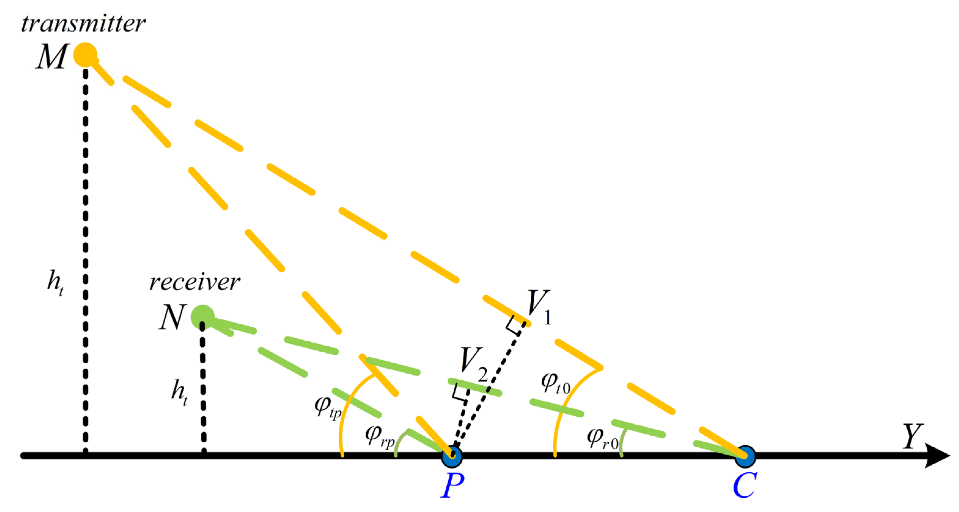
2. HS-BFSAR Signal Model and Range Doppler Spectrum

The imaging geometry graph in Figure 1 exhibits the configuration of spaceborne HS-BFSAR. The transmitter and the receiver are, respectively, placed in the satellite and the high-speed platform, and they are located at $M\left(0,y_t,h_t\right)$ and $N\left(0,0,h_r\right)$ in the synthetic aperture center time. The sub-satellite point of the transmitter is located at $O_t$. The heights of the transmitter and receiver are $h_t$ and $h_r$, respectively. The projection point of the receiver on the ground is $O_r$, which is taken as the origin of the right-hand Cartesian coordinate system. The transmitter travels along the $X$ axis with a velocity of $v_t$, and the velocity of the receiver is $v_r$. The extension line of $v_r$ meets the ground at $C$, which serves as the center of the imaging scene. The angle between the line $MC$ and the ground is ${\phi }_{t0}$, while the angle between the line $NC$ and the ground is ${\phi }_{r0}$. $P\left(x_p,y_p\right)$ is an arbitrary point target in the imaging scene. We assume that there is no phase error in the system after using direct signal synchronization [49] because phase synchronization is not the focus of this paper. In addition, for HS-BFSAR, the imaging area is not very large, so the curvature of the Earth is not considered in this paper. Assuming that the transmitted signal is a linear-frequency-modulated (LFM) pulse, the received signal after demodulation can be expressed as

$$s\left(t,t_a;x_p,y_p\right)=w_r\left(t-t_b\right)w_a\left(t_a-t_n\right)\exp \left(j\pi \gamma {\left(t-t_b\right)}^2\right)\exp \left(-j\frac{2\pi }{\lambda }{R}_{bf}\left(t_a;x_p,y_p\right)\right)$$

(1)

where $w_r$ and $w_a$ are the range and azimuth envelopes, respectively. $t$ is the fast time and $t_a$ is the slow time. $\lambda$ is the wavelength, which is the ratio of the speed of light $c$ to carrier frequency $f_c$. $\gamma$ represents the range FM rate. In addition, $t_b$ is the bistatic range of point $P$ at $t_a$ and $t_n$ is the azimuthal time position, which can be expressed as

$$t_b=\frac{R_{bf}\left(t_a;x_p,y_p\right)}{c}\hspace{1em}{t}_n=\frac{x_p}{v_t}$$

(2)

where $R_{bf}\left(t_a;x_p,y_p\right)$ is the bistatic range history, which is given by

$$R_{bf}\left(t_a;x_p,y_p\right)=\sqrt{{\left(v_t{t}_a-x_p\right)}^2+{\left(y_t-y_p\right)}^2+h_t^2}+\sqrt{x_p^2+{\left(v_{ry}{t}_a-y_p\right)}^2+{\left(h_r-v_{rz}{t}_a\right)}^2}$$

(3)

where $v_{ry}$ and $v_{rz}$ are components of $v_r$ in the $Y$ and $Z$ directions, respectively.

The bistatic range history has a double-squared-root (DSR) term, which makes it difficult to derive an analytical expression of the bistatic 2D spectrum. The method of series reversion (MSR) can solve the 2D spectrum of any BiSAR configuration [29]. However, the classical MSR cannot directly solve the bistatic range Doppler spectrum in HS-BFSAR, which is very important for the range NLCS operation. To derive the HS-BFSAR range Doppler spectrum, we first simplify the bistatic range history in (3). The detection range of the high-speed platform receiver is generally close to one hundred kilometers. In the imaging scene of several kilometers, the receiving beam can be regarded as a plane wave. Therefore, the velocity of the receiver relative to point $P$ is equivalent to $v_r$, based on the plane wave assumption (PWA). At the same time, the range history of the transmitter is replaced by an equivalent quadratic model. Based on the above assumptions, the equivalent bistatic range history can be written as

$${R^{\prime }}_{bf}\left(t_a;x_p,y_p\right)=R_{bf0}\left(x_p,y_p\right)-v_r{t}_a+\frac{v_t^2{t}_a^2}{2R_{t0}\left(x_p,y_p\right)}$$

(4)

where

$$R_{bf0}\left(x_p,y_p\right)=R_{t0}\left(x_p,y_p\right)+R_{r0}\left(x_p,y_p\right)$$

(5)

$$R_{t0}\left(x_p,y_p\right)=\sqrt{x_p^2+{\left(y_t-y_p\right)}^2+h_t^2}$$

(6)

$$R_{r0}\left(x_p,y_p\right)=\sqrt{x_p^2+y_p{}^2+h_r^2}$$

(7)

Figure 2 shows the ranging model error and its phase error represented by the Equation (4) under the parameters in

Table 1. Spaceborne HS-BFSAR simulation parameters.

Parameter	Transmitter	Receiver
Height	750 km	10 km
Velocity	7000 m/s	1000 m/s
Max detection range	757 km	51 km
Carrier band	C
Pulse repetition frequency	2000 Hz
Range bandwidth	150 MHz
Synthetic aperture time	2 s

. Obviously, in the whole synthetic aperture time, the phase error is less than the tolerance limit of phase coherence, which is $0.25\pi \left(rad\right)$ [1]. Using the principle of stationary phase (POSP) [51] and MSR [29], the two-dimensional spectrum of the received signal can be derived and then expanded it to the cubic term of $f_r$, which is given by

$$\begin{array}{cc}S\left(f_r,f_a;x_p,y_p\right)& =W_r\left(f_r\right)W_a\left(f_a\right)\exp \left(j\left(-2\pi \frac{f_c{R}_{bf0}}{c}+\pi \frac{{\left(c{f}_a-v_r{f}_c\right)}^2{R}_{t0}}{c{v}_t{}^2{f}_c}\right)\right)\\ & \times \exp \left(j\left(-2\pi \frac{R_{bf0}}{c}+\pi \frac{v_r^2{R}_{t0}}{c{v}_t{}^2}-\pi \frac{c{R}_{t0}{f}_a^2}{v_t{}^2{f}_c^2}\right)f_r\right)\\ & \times \exp \left(j\left(\pi \left(-\frac{1}{\gamma }+\frac{c{R}_{t0}{f}_a^2}{v_t^2{f}_c^3}\right)f_r^2-\pi \frac{c{R}_{t0}{f}_a^2}{v_t^2{f}_c^4}{f}_r^3\right)\right)\end{array}$$

(8)

where $f_r$ and $f_a$ are the range frequency and the azimuth frequency, respectively.

After the range inverse Fourier transform, we can obtain the expression of the signal in the range-Doppler domain as follows

$$\begin{array}{cc}S\left(t,f_a;x_p,y_p\right)& =W_r\left(t\right)W_a\left(f_a\right)\exp \left(j\left(-2\pi \frac{f_c{R}_{bf0}}{c}+\pi \frac{v_r^2{f}_c{R}_{t0}}{c{v}_t^2}+\pi \frac{\gamma v_r^4{R}_{t0}^2}{4c^2{v}_t^4}\right)\right)\\ & \times \exp \left(j\left(-2\pi \frac{v_r{R}_{t0}}{v_t^2}{f}_a+\pi \left(\frac{{\gamma }^2{v}_r^4{R}_{t0}^3}{4c{v}_t^6{f}_c^3}-\frac{\gamma v_r^2{R}_{t0}^2}{2v_t^4{f}_c^2}+\frac{c{R}_{t0}}{v_t^2{f}_c}\right)f_a^2\right)\right)\\ & \times \exp \left(j\left(\begin{array}{l}\pi \left(\left(\frac{{\gamma }^2{v}_r^2{R}_{t0}^2}{v_t^4{f}_c^3}-\frac{\gamma c{R}_{t0}}{v_t^2{f}_c^2}\right)f_a^2+\frac{\gamma v_r^2{R}_{t0}}{c{v}_t^2}\right)\left(t-\frac{R_{bf0}}{c}\right)\\ +\pi \left(\gamma +\frac{c{\gamma }^2{R}_{t0}{f}_a^2}{v_t^2{f}_c^3}\right){\left(t-\frac{R_{bf0}}{c}\right)}^2\end{array}\right)\right)\end{array}$$

(9)

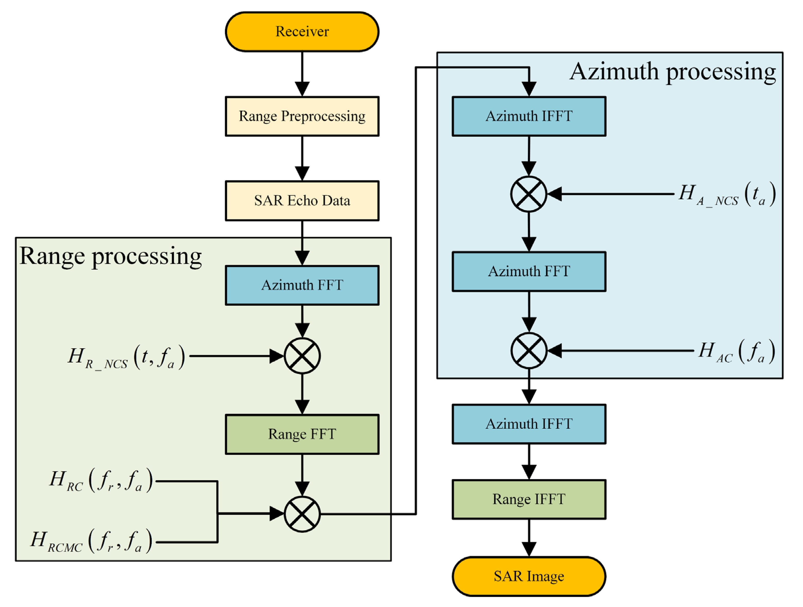
3. Range Preprocessing and Range NLCS

In this section, we focus on how to implement RCMC and range compression with the help of range preprocessing and NLCS. Range preprocessing can greatly alleviate the range–azimuth coupling of the RCM, while range NLCS can equalize the RCM and range FM rate.

3.1. Range Preprocessing in Echo Recording

In HS-BFSAR, the receiver has a high forward speed, which increases the range cell span of the target echo in the whole synthetic aperture time. This means that the echo of the edge target cannot be fully recorded. The automatic range gate (ARG) is proposed in this paper to solve this problem. Previously based on the PWA, it is seen that there is a huge linear component in the time delay of the echo signal from transmitting to receiving. Suppose that $t_{start}$ is the starting time of the range gate, then $t_{start}$ and $t_a$ have the following relation

$$t_{start}=\frac{1}{c}\left(R_{bf0\_ref}-\frac{W_d}{2}-v_r{t}_a\right)$$

(10)

where $R_{bf0\_ref}$ is $R_{bf0}$ at the reference point, selecting the point $C$ in the center of the scene as the reference point. $W_d$ is the width of the range gate, depending on the size of the scene echo. In order to highlight the benefits of ARG, we compare the echo data with and without range preprocessing. The simulation results are shown in Figure 3. In addition to point $C$, we have two points along the $Y$ axis that are three kilometers from point $C$. We can see in Figure 3a that the echo of the target at the edge point exceeds the range gate at some azimuth sampling times and is not received. Figure 3b shows the echo data after range preprocessing, demonstrating that all the echoes of the target at the edge point can be recorded.

After the range preprocessing of ARG, it cannot only record echo data with a wider swath but also reduce the demand for range sampling points, which is conducive to the fast imaging of the high-speed platform receiver. Even for general bistatic forward-looking SAR, RCM is still dominated by linear RCM. Range preprocessing can greatly reduce but not completely remove the coupling between range and azimuth. Thereby, in Section 3.2, the range NLCS algorithm is proposed to solve this problem.

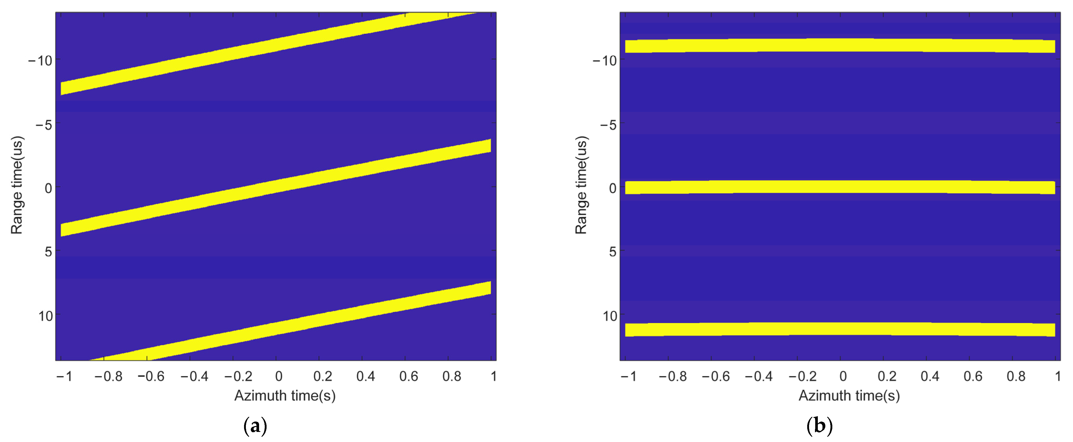
3.2. RCMC and Range Compression Using NLCS

After the range preprocessing, the coupling between the range and azimuth of the RCM is greatly reduced, but the space-variant residual RCM will make the range compressed echo of the target scattered in several range units, which is unfavorable for imaging. A range NLCS is proposed to solve the above problem in this subsection. Figure 4 shows the principle of equalizing the quadratic phase using the cubic perturbation function, which can describe the influence of the introduction of the NLCS factor on the signal phase. Figure 4b shows that the echo signals of targets $P_{-}$, $P_0$, $P_{+}$ with different quadratic phase parameters that can be adjusted to the uniform quadratic phase curvature after introducing the cubic perturbation function in the time domain. Then, the echo signals of these targets can be uniformly phase-filtered in the frequency domain. Therefore, using the NLCS factor can eliminate the spatial variation of the phase to a certain extent, which is discussed in detail below.

From (8) and (9), the phase terms of RCM and the effective range FM rate can be expressed as

$${\Phi }_{RCM}=-\pi \frac{c{R}_{t0}}{v_t^2{f}_c^2}{f}_a^2{f}_r$$

(11)

$${\gamma }_e=\gamma +\frac{c{\gamma }^2{R}_{t0}}{v_t^2{f}_c^3}{f}_a^2$$

(12)

where ${\Phi }_{RCM}$ is the linear phase term of $f_r$ and ${\gamma }_e$ is the effective range FM rate. ${\Phi }_{RCM}$ makes the envelope of the target echo present a curved shape after range compression.

In (12), it can be seen that the original range FM rate becomes the additional secondary azimuth frequency term effective range FM rate, and its spatial variation is the main cause of range defocus. From the expressions of ${\Phi }_{RCM}$ and ${\gamma }_e$, we comprehend that the spatial variation of RCM and ${\gamma }_e$ lies in $R_{t0}$. Therefore, the analysis of $R_{t0}$ is the basis of eliminating the above spatial variation. Figure 5 shows the distribution of $R_{t0}$ and $R_{bf0}$, simulating in a large scene and setting the reference point as the origin of the coordinates. It can be seen that, although $R_{t0}$ and $R_{bf0}$ are variational in two dimensions, they mainly change along the $Y$ axis. Therefore, in this paper, the $Y$ axis is defined as the range direction, while the $X$ axis is defined as the azimuth direction. Based on the above analysis, we believe that the spatial variation of RCM, and ${\gamma }_e$ are mainly in the range direction, and it is difficult to remove their spatial variation along the azimuth direction [42].

To solve the spatial variation with range, we used the imaging geometry in Figure 6 for analysis. In Figure 6, $P{V}_1$ and $P{V}_2$ are the vertical lines of $CM$ and $CN$, respectively, ${\phi }_{tp}$ and ${\phi }_{rp}$ are the angles of $PM$ and $PN$ with the $Y$ axis, respectively. In spaceborne HS-BFSAR, the detection range is much larger than the imaging scene size, so $M{V}_1$ and $N{V}_2$ can be approximated as $MP$ and $NP$, respectively. $MP$ and $NP$ represent $R_{t0}$ and $R_{r0}$, respectively. Then, the range of point $P$ can be expressed as

$$\begin{array}{cc}{R}_{bf0}& =MP+NP\\ & \approx \left(MC-M{V}_1\right)+\left(NC-NP\right)\end{array}$$

(13)

Using a simple geometric relationship, we can obtain

$$\Delta R_{r0}=\alpha ·\Delta R_{t0}$$

(14)

where

$$\Delta R_{t0}=R_{t0}-R_{t0\_ref}$$

(15)

$$\Delta R_{r0}=R_{r0}-R_{r0\_ref}$$

(16)

where $R_{t0\_ref}$ and $R_{r0\_ref}$ are the $R_{t0}$ and $R_{r0}$ at the reference point, respectively. $\alpha$ is the ratio of $\cos {\phi }_{r0}$ to $\cos {\phi }_{t0}$. Thus, we can obtain the equation of $R_{t0}$ in $\Delta t_0$ as

$$R_{t0}=R_{t0\_ref}+\frac{c·\Delta t_0}{\alpha +1}$$

(17)

where

$$\Delta t_0=t_0-t_{0\_ref}$$

(18)

where $t_0$ and $t_{0\_ref}$ is the focusing time of point $P$ and the reference point, respectively.

Then, we use NLCS to equalize the range-dependent spatial variation of RCM and range FM rate. We introduce the NLCS factor in the range-Doppler domain of the echo signal. The NLCS factor is expressed as

$$H_{R\_NCS}\left(t,f_a\right)=\exp \left\{j\pi q_2{\left(t-t_{0\_ref}\right)}^2+j\pi q_3{\left(t-t_{0\_ref}\right)}^3\right\}$$

(19)

After multiplying (9) by (19) and expanding $t$ at $t_0$ to its cubic Taylor series, the range-modulated phase can be written as

$${\Phi }_R\left(t,f_a\right)=\pi \hspace{0.17em}{\Phi }_{R0}\left(f_a\right)+\pi \hspace{0.17em}{\Phi }_{R1}\left(f_a\right)·\left(t-t_0\right)+\pi \hspace{0.17em}{\Phi }_{R2}\left(f_a\right)·{\left(t-t_0\right)}^2+\pi \hspace{0.17em}{q}_3·{\left(t-t_0\right)}^3$$

(20)

where

$$\begin{array}{cc}{\Phi }_{R0}& =\left(\frac{{\gamma }^2{v}_r^4{R}_{t0}^3}{4c{v}_t^6{f}_c{}^3}-\frac{\gamma v_r^2{R}_{t0}^2}{2v_t^4{f}_c{}^2}+\frac{c{R}_{t0}}{v_t^2{f}_c}\right)f_a^2-2\frac{v_r{R}_{t0}}{v_t^2}{f}_a\\ & -2\frac{f_c\left(R_{t0}+R_{r0}\right)}{c}+\frac{v_r^2{f}_c{R}_{t0}}{c{v}_t^2}+\frac{\gamma v_r^4{R}_{t0}^2}{4c^2{v}_t^4}+q_2\Delta t_0^2+q_3\Delta t_0^3\end{array}$$

(21)

$${\Phi }_{R1}=\left(\frac{{\gamma }^2{v}_r^2{R}_{t0}^2}{v_t^4{f}_c^3}-\frac{c\gamma R_{t0}}{v_t^2{f}_c^2}\right)f_a^2+\frac{\gamma v_r^2{R}_{t0}}{c{v}_t{}^2}+2q_2\Delta t_0+3q_3\Delta t_0^2$$

(22)

$${\Phi }_{R2}=\frac{c{\gamma }^2{R}_{t0}}{v_t^2{f}_c^3}{f}_a^2+\gamma +q_2+3q_3\Delta t_0$$

(23)

Substituting (17) into (22) and (23), and letting the spatial variation term containing $\Delta t_0$ be zero, the coefficients $q_2$ and $q_3$ can be written as

$$q_2=\frac{\left(2c{\gamma }^2{v}_r^2{R}_{t0\_ref}-c^2\gamma v_t^2{f}_c\right)f_a^2+\gamma v_r^2{v}_t^2{f}_c^3}{2\left(\alpha +1\right)v_t^4{f}_c^3}$$

(24)

$$q_3=\frac{c^2{\gamma }^2{v}_r^2{f}_a^2}{3{\left(\alpha +1\right)}^2{v}_t^4{f}_c^3}$$

(25)

Next, a range Fourier transform is performed. The range-modulated phase in the frequency domain is expressed as

$${\Phi }_F\left(f_r,f_a\right)=\pi \hspace{0.17em}{\Phi }_{F0}+\pi \hspace{0.17em}\left(2t_0+{\Phi }_{F1}\right)f_r+\pi \hspace{0.17em}{\Phi }_{F2}{f}_r^2+\pi \hspace{0.17em}{\Phi }_{F3}{f}_r^3$$

(26)

The coefficients of phase ${\Phi }_{F0}$, ${\Phi }_{F1}$, ${\Phi }_{F2}$, ${\Phi }_{F3}$ are presented in Appendix A. Therefore, the RCMC filter and the range compression filter be written as

$$H_{RCMC}=\exp \left(-j\pi \hspace{0.17em}{\Phi }_{F1}{f}_r\right)$$

(27)

$$H_{RC}=\exp \left(-j\pi \left({\Phi }_{F2}{f}_r^2+{\Phi }_{F3}{f}_r^3\right)\right)$$

(28)

To illustrate the advantage of the proposed algorithm to the traditional NLCS algorithm [40], we arrange the target $P_{-}$ and target $P_{+}$ in the imaging scene. $P_{-}$ and $P_{+}$ are placed on both sides of the reference point on the $Y$ axis, 5 km away from the reference point. Figure 7 shows the results of the range processing by the traditional NLCS algorithm and the proposed method, and proves that the proposed method can effectively focus the echo signal within a range cell.

4. Azimuth Compression via Modified NLCS

After the range processing, the echo signal of the target can be concentrated within a range cell. This section aims at performing the azimuth compression of the echo signal to accomplish the focusing of the echo signal. In SAR signal processing, the azimuth signal is also considered a frequency modulation signal. The azimuth FM rate and the azimuth cubic FM rate are, respectively, defined as $K_a$ and $K_t$, which can be expressed as

$$K_a=-\frac{2}{\lambda }·\frac{d^2{R}_{bf}\left(t_a\right)}{d{t}_a^2}$$

(29)

$$K_t=-\frac{2}{\lambda }·\frac{d^3{R}_{bf}\left(t_a\right)}{d{t}_a^3}$$

(30)

Figure 8 shows the distribution of $K_a$ and $K_t$ in the scene, and the origin of the coordinates is the reference point. It can be seen that $K_a$ is a two-dimensional space-variant, which makes the azimuth signal difficult to focus. Unlike $K_a$, the value of $K_t$ is particularly small throughout the scene. Thus, $K_t$ is not discussed separately in this paper. The spatial variation of $K_a$ will be analyzed in detail in the following.

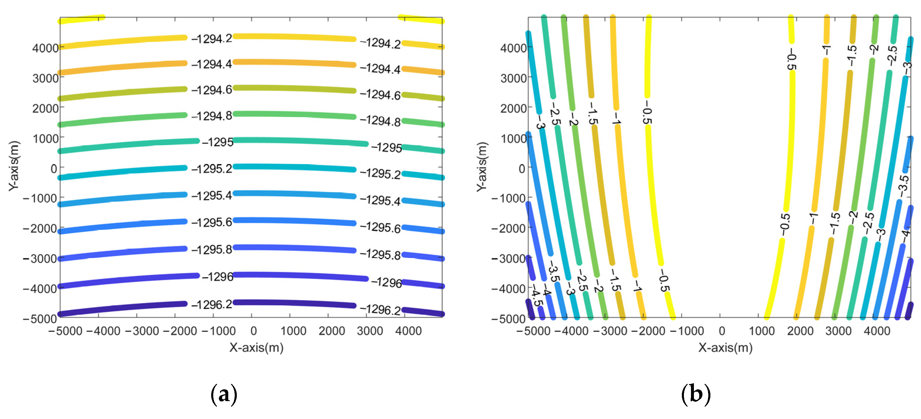
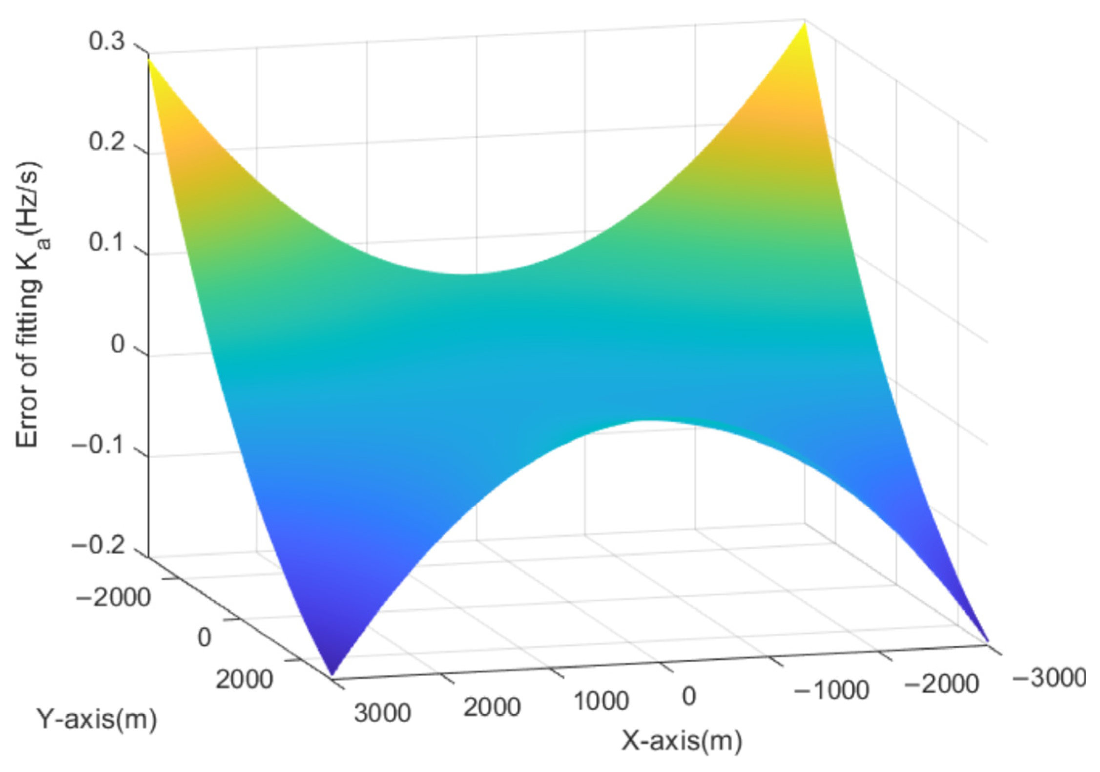
4.1. Analysis of Azimuth FM Rate

The azimuth FM rate is the modulation of the echo signal about $t_a$ caused by the Doppler effect of the moving platform. In [1], the azimuth FM rate is expressed as a linear function of the $t_a$ derivative of the range history. In BiSAR, the range history can be decomposed into the range history of the transmitter and the range history of the receiver. Therefore, $K_a$ can be decomposed as follows

$$\begin{array}{cc}{K}_a& =-\frac{2}{\lambda }·\frac{d^2\left(R_t\left(t_a\right)+R_r\left(t_a\right)\right)}{d{t}_a^2}\\ & =-\frac{2}{\lambda }·\frac{d^2{R}_t\left(t_a\right)}{d{t}_a^2}-\frac{2}{\lambda }·\frac{d^2{R}_r\left(t_a\right)}{d{t}_a^2}\\ & =K_{at}+K_{ar}\end{array}$$

(31)

where the $K_{at}$ and $K_{ar}$ are the azimuth FM rate introduced by the transmitter motion and the receiver motion, respectively. $R_t\left(t_a\right)$ and $R_r\left(t_a\right)$ are the range history of the transmitter and the range history of the receiver, respectively.

Figure 9 shows the distribution of $K_{at}$ and $K_{ar}$ in the scene. It can be seen that they mainly change along the $Y$ axis and $X$ axis directions, respectively. Thus, it can be concluded that $K_{at}$ is a range-dependent spatial variational and $K_{ar}$ is the azimuth-dependent spatial variational. This means that we can eliminate the spatial variational of $K_a$ from the range and azimuth dimensions, respectively.

In Figure 10, the imaging geometry is separated into the configuration in which the radar signal is transmitted and the configuration in which the echo signal is received. We placed the point $P_Y$ on the $Y$ axis and the point $P_X$ on the same $Y$ axis as the reference point. ${\varphi }_r$ is the angle between $NC$ and $N{P}_X$. To apply the above geometric relationship to derive $K_{at}$ and $K_{ar}$, the azimuth FM rate in monostatic SAR is introduced, which can be written as

$$K_{a\_mono}=-\frac{2V^2{\sin }^2\left(\varphi \right)}{\lambda R}$$

(32)

where $\varphi$ is the angle between the direction of the velocity $V$ and the slant range $R$. Considering the single-range propagation of the transmitted signal, $K_{at}$ can be expressed as

$$K_{at}=-\frac{v_t^2}{\lambda R_{t0}}$$

(33)

From (33), we can find that the spatial variation of $K_{at}$ is due to $R_{t0}$, which can be represented with (17). For the azimuth-dependent spatial variation of $K_{ar}$, we used $t_n$ to describe it. In Figure 10b, we have

$$\sin \left({\varphi }_r\right)=\frac{v_t{t}_n}{R_{r0}}$$

(34)

where

$$R_{r0}=\sqrt{R_{r0\_ref}^2+{\left(v_t{t}_n\right)}^2}$$

(35)

where $R_{r0\_ref}$ is the $R_{r0}$ at the reference point. From (32), (34), and (35), $K_{ar}$ can be expressed with $t_n$. We use a Taylor expansion of $t_n$ to facilitate the subsequent analysis later, and $K_{ar}$ can be written as

$$K_{ar}=-\frac{v_r^2{v}_t^2}{\lambda R_{r0}^3}·t_n^2+\frac{3v_r^2{v}_t^4}{2\lambda R_{r0}^5}·t_n^4$$

(36)

Then, the two-dimensional fitting $K_{a\_fit}$ can be expressed as

$$K_{a\_fit}=-\frac{\left(\alpha +1\right)v_t^2}{\lambda \left(\left(\alpha +1\right)R_{t0\_ref}+c·\Delta t_0\right)}-\frac{v_r^2{v}_t^2}{\lambda R_{r0}^3}·t_n^2+\frac{3v_r^2{v}_t^4}{2\lambda R_{r0}^5}·t_n^4$$

(37)

The difference between $K_{a\_fit}$ and $K_a$ is shown in Figure 11. The max quadratic phase error (QPE) is $0.295\pi$, which is lower than the limit value of the 5%-spread impact response width (IRW) [1].

4.2. Azimuth FM Rate Equalizing by Modified NLCS

Since the range and azimuth directions of the echo signal are decoupled in the range processing, the spatial variation of the azimuth FM rate along the range direction can be equalized by a filter with range variation. The azimuth NLCS factor is given as follows

$$H_{A\_NCS}=\exp \left\{j\pi p_4{t}_a^4+j\pi p_6{t}_a^6\right\}$$

(38)

Multiplying (38) by the azimuth quadratic FM phase and expanding at $t_n$ to the cubic term of $t_a$, the phase can be written as

$${\Phi }_A\left(t_a\right)=\pi \hspace{0.17em}{\Phi }_{A0}+\pi \hspace{0.17em}{\Phi }_{A1}\left(t_a-t_n\right)+\pi \hspace{0.17em}{\Phi }_{A2}{\left(t_a-t_n\right)}^2+\pi \hspace{0.17em}{\Phi }_{A3}{\left(t_a-t_n\right)}^3$$

(39)

where

$${\Phi }_{A0}=\left(-\frac{v_{r0}^4{t}_n^2}{R_{r0}^3\lambda }+\frac{3v_{r0}^6{t}_n^4}{2R_{r0}^5\lambda }+K_{at}\right)t_n^2+p_6{t}_n^6+p_4{t}_n^4$$

(40)

$${\Phi }_{A1}=2\left(-\frac{v_{r0}^4{t}_n^2}{R_{r0}^3\lambda }+\frac{3v_{r0}^6{t}_n^4}{2R_{r0}^5\lambda }+K_{at}\right)t_n+6p_6{t}_n^5+4p_4{t}_n^3$$

(41)

$${\Phi }_{A2}=-\frac{v_{r0}^4{t}_n^2}{R_{r0}^3\lambda }+\frac{3v_{r0}^6{t}_n^4}{2R_{r0}^5\lambda }+K_{at}+15p_6{t}_n^4+6p_4{t}_n^2$$

(42)

$${\Phi }_{A3}=20p_6{t}_n^3+4p_4{t}_n$$

(43)

To make the term of $t_n$ in (42) be zero, we have

$$p_4=\frac{v_r^2{v}_t^2}{6\lambda R_{r0}^3}$$

(44)

$$p_6=-\frac{v_r^2{v}_t^4}{10\lambda R_{r0}^5}$$

(45)

To date, the space-variant $K_{ar}$ is equalized, and the azimuth compression can be performed uniformly in the azimuth frequency domain. The azimuth compression filter can be expressed as

$$H_{ac}=\exp \left(-j\pi \frac{\lambda \left(\alpha +1\right)R_{t0\_ref}+c·\Delta t_0}{\left(\alpha +1\right)v_t^2}{f}_a^2\right)$$

(46)

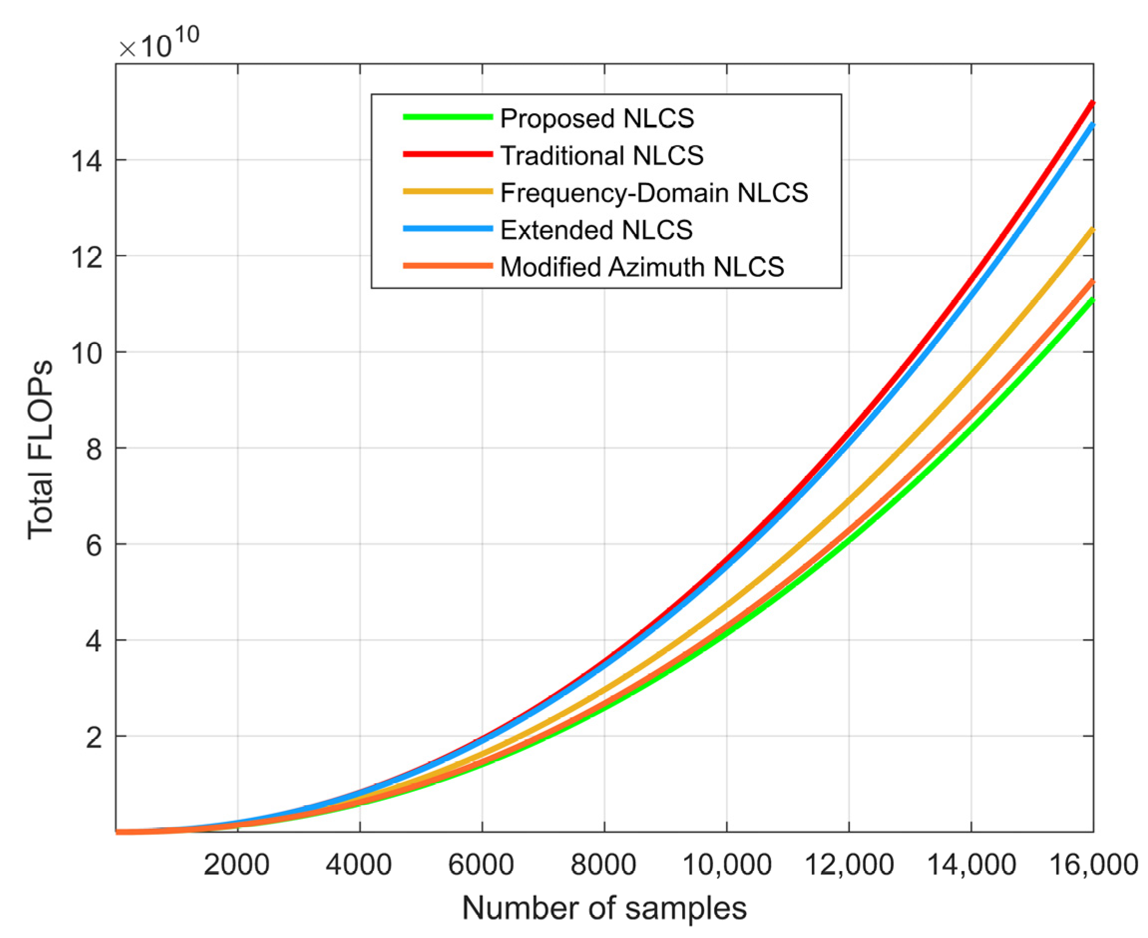
4.3. Computing Burden of Proposed Algorithm

For HS-BFSAR, real-time imaging is necessary. Therefore, under the premise of adequate imaging quality, the algorithm requires less computing burden. Figure 12 shows the block diagram of the proposed algorithm. The floating-point operations (FLOPs) of a $N$-point FFT or IFFT and one-time complex multiplication are $5N{\log }_{2}N$ and $6N$ [52], respectively. Thus, the total FLOPs of the proposed algorithm can be written as

$$C_{Proposed algorithm}=24N_r{N}_a+20N_r{N}_a{\log }_2{N}_a+10N_r{N}_a{\log }_2{N}_r$$

(47)

We choose the traditional NLCS algorithm [40] and several typical NLCS algorithms [22,43,53] for the comparison of the computing burden. The total FLOPs of these algorithms can be written as

$$C_{Traditional NLCS}=36N_r{N}_a+20N_r{N}_a{\log }_2{N}_a+20N_r{N}_a{\log }_2{N}_r$$

(48)

$$C_{Frequency-Domain\hspace{0.17em}NLCS}=30N_r{N}_a+15N_r{N}_a{\log }_2{N}_a+10N_r{N}_a{\log }_2{N}_r+2\left(2M-1\right)N_r{N}_a$$

(49)

$$C_{Extended\hspace{0.17em}NLCS}=30N_r{N}_a+20N_r{N}_a{\log }_2{N}_a+10N_r{N}_a{\log }_2{N}_r+2\left(2M-1\right)N_r{N}_a$$

(50)

$$C_{Modified\hspace{0.17em}Azimuth\hspace{0.17em}NLCS}=30N_r{N}_a+20N_r{N}_a{\log }_2{N}_a+10N_r{N}_a{\log }_2{N}_r$$

(51)

where $N_r$ and $N_a$ are the number of the range and azimuth samples, respectively. $M$ is the number of neighbor samples used for the range and azimuth interpolation.

Figure 13 shows the relative values of the computational burden of these algorithms to that of the proposed algorithm. To intuitively reflect the simulation results, $N_r$ and $N_a$ are set to the same size, and the value of $M$ is 16. The results show that the proposed algorithm has the least computing burden along the mentioned NLCS algorithms.

5. Simulation Results and Discussion

In this section, the effectiveness of the proposed method is verified by the point simulation and scene simulation. To get closer to the characteristics of the spaceborne HS-BFSAR, the Gaofen-3 satellite is referred to as the transmitter, while the high-speed receiver is looking forward to the scene on the ground. The specific simulation parameters are given in Table 1. In addition, the traditional NLCS algorithm proposed by Wong et al. [40] is taken as a conventional method, and Mei’s frequency-domain NLCS algorithm [22] is used as a reference method.

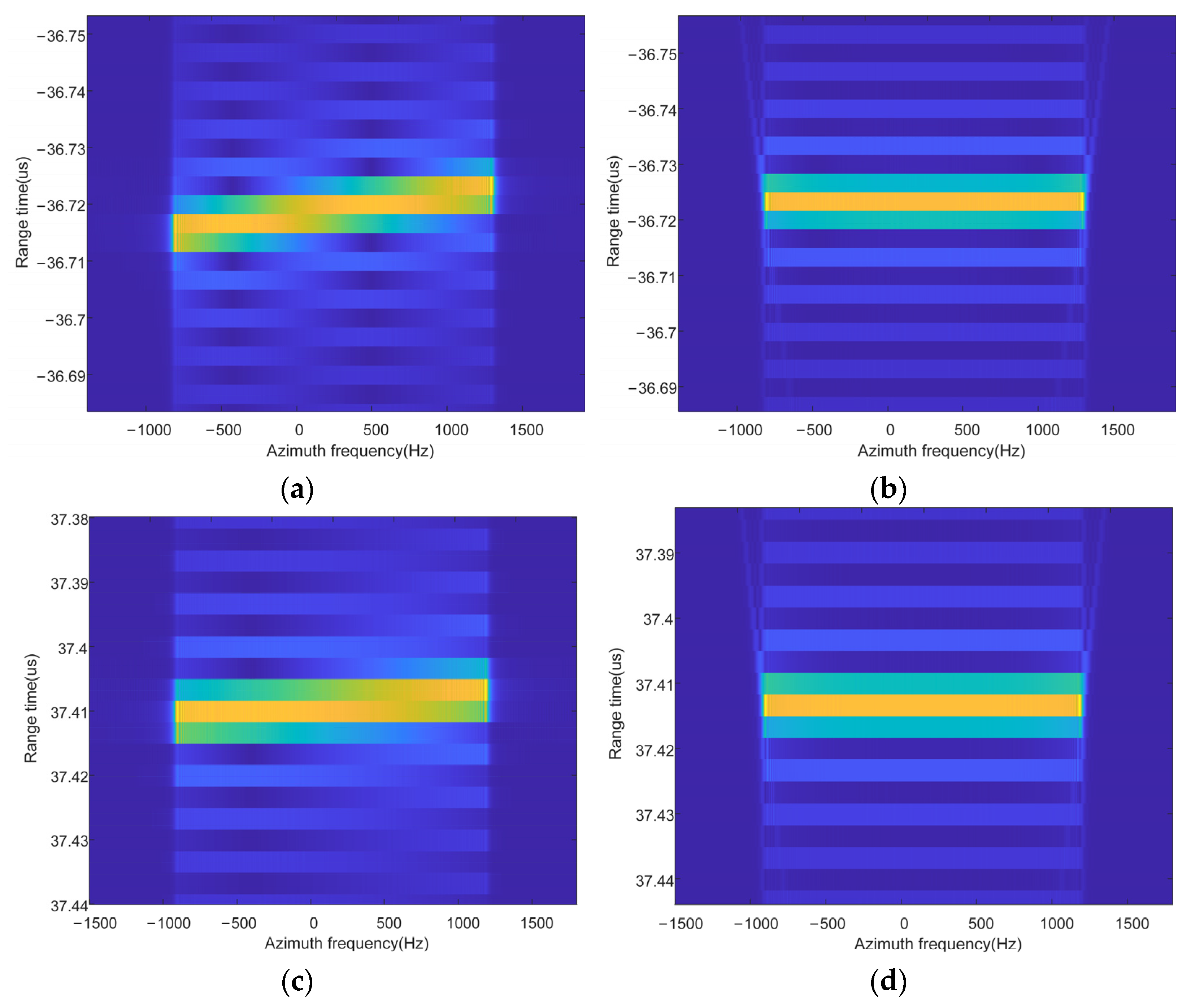
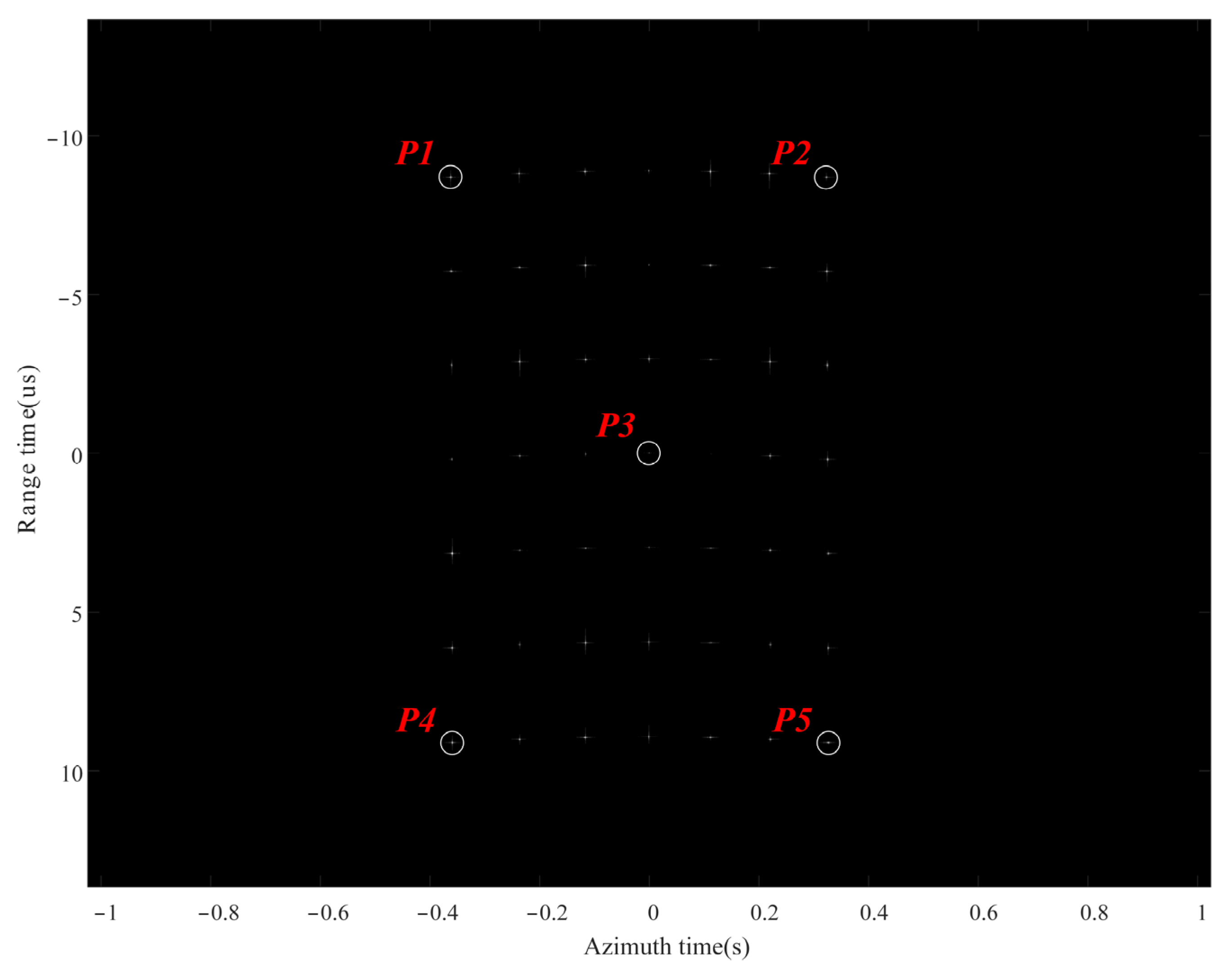
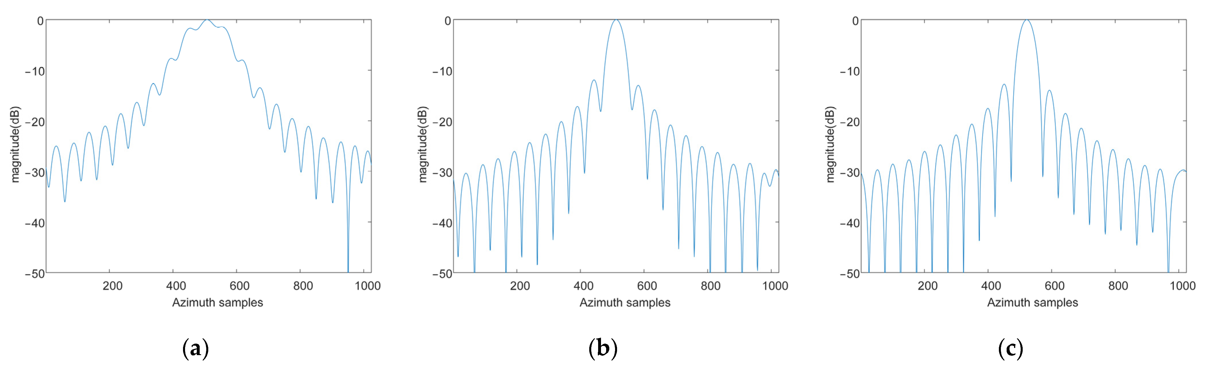
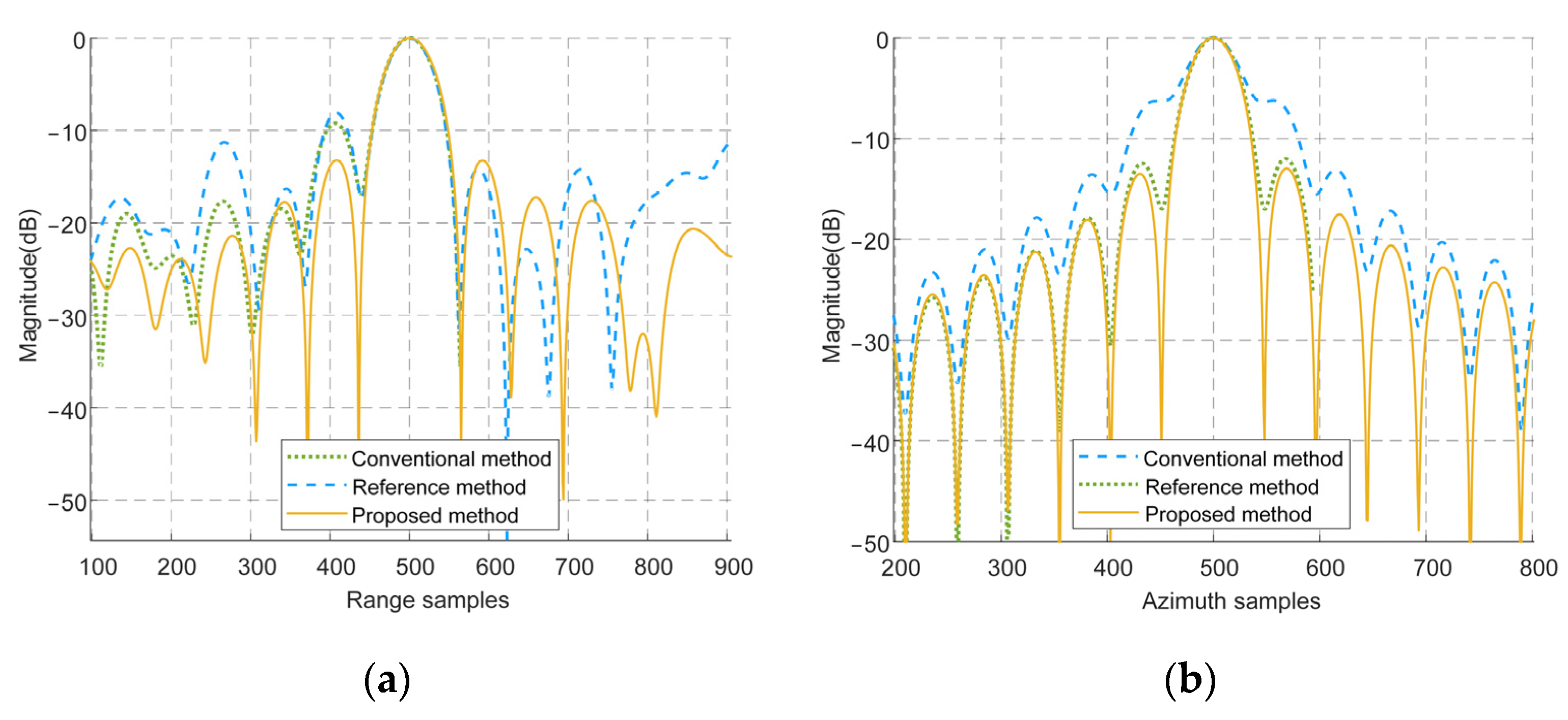
5.1. Results of Point Simulation

The point simulation uses an array of 49 targets, which are distributed in a 4.8 km² grid in the ground range and azimuth. The original imaging results are shown in Figure 14, where point P3 is the scene reference point and the remaining marked points are the scene edge points. The detailed imaging results of points P1, P3, and P5 are shown in Figure 15, Figure 16, Figure 17, Figure 18, Figure 19 and Figure 20 in contrast with the results of the conventional method and the reference method.

Figure 15 and Figure 18 gives the contour plots of the selected points using the different algorithms, which demonstrates the 2D focusing performance. From Figure 16a, Figure 17a, Figure 18a, Figure 19a and Figure 20a, it can be seen that the main lobe of the result using the conventional method [40] is widened, especially in the azimuth. This is because the conventional method [40] does not consider the spatial variation of RCM and the high-order spatial variation of the azimuth FM rate, so it cannot deal with the BFSAR configuration. The reference method [22] corrects the linear RCM and equalizes the Doppler parameters by introducing a KT transform and a frequency-domain NLCS, respectively. However, the reference method [22] ignores the spatial variation of range curvature and range FM rate in the scene, resulting in an increase in the side lobe of the range profile, which is shown in Figure 16b and Figure 19b. In addition, the reference method [22] does not consider the high-order spatial variation of the azimuth FM rate, which leads to a broadening of the azimuth profile in Figure 17b and Figure 20b. The measured performances of targets P1, P3, and P5 are listed in

Table 2. Measured parameters of the selected targets. PSLR: peak sidelobe ratio; and ISLR: integrated sidelobe ratio.

Method	Targets	Range		Azimuth
		PSLR (dB)	ISLR (dB)	PSLR (dB)	ISLR (dB)
Conventional method	P1	−12.56	−9.82	N/A	N/A
	P3	−13.23	−10.25	−13.24	−9.86
	P5	−12.15	−9.64	N/A	N/A
Reference method	P1	−12.99	−9.76	−6.96	−7.04
	P3	−13.23	−10.25	−13.24	−9.86
	P5	−12.25	−9.79	−11.34	−8.62
Proposed method	P1	−13.21	−10.12	−13.21	−9.74
	P3	−13.23	−10.25	−13.24	−9.86
	P5	−13.23	−10.25	−13.23	−9.86

. Inspecting Table 2, it can be found that the 2D measured parameters obtained by the proposed algorithm are close to the theoretical values. However, the parameters of the conventional method [40] and the reference method [22] are worse compared to the proposed method.

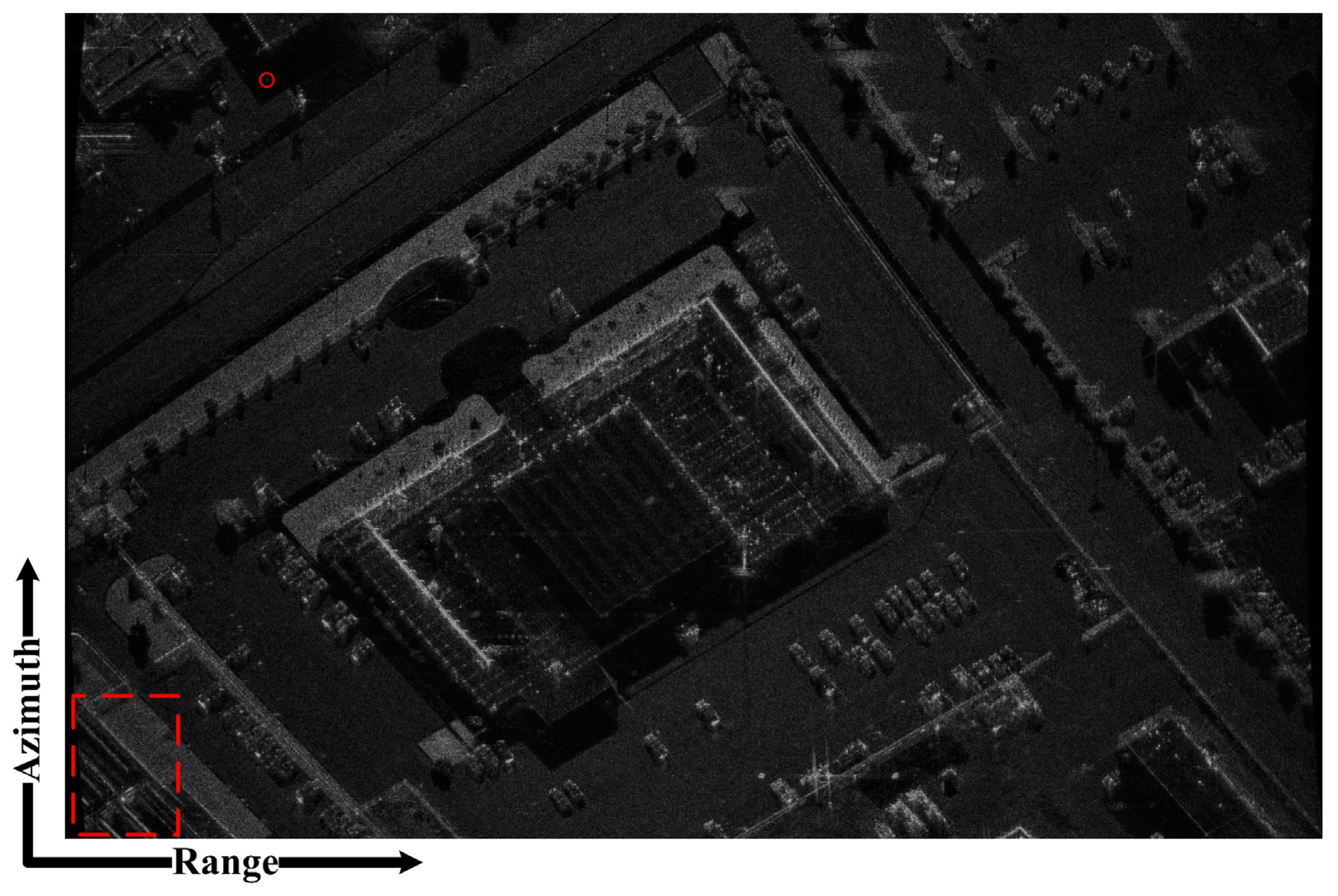
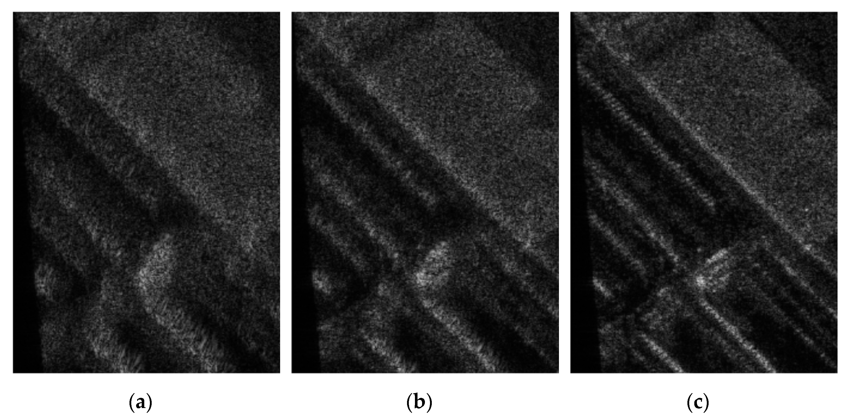
5.2. Results of Scene Simulation

To further prove the effectiveness of the proposed method in the complex imaging scene, a scene target is simulated based on a benchmark SAR image. In the scene simulation, each pixel of the benchmark SAR image is regarded as a scattering point of the scene target. The intervals between each scattering point and the size of the scene target are 2 m and 5 × 5 km, respectively. Figure 21 shows the imaging results of the scene target processed by the proposed method.

It can be seen that the scattering characteristics of the benchmark SAR images are well displayed by the processing of the proposed method. However, in Figure 22a,b, the images processed by the conventional method [40] and the reference method [22] are defocused to varying degrees, respectively. For a more intuitive comparison, an isolated edge point at the red dashed circle in Figure 21 is selected, and the corresponding range and azimuth profiles via the three methods are shown in Figure 23. Similarly to the point simulation, the conventional method [40] and the reference method [22] are not suitable for imaging in spaceborne HS-BFSAR configuration, which leads to the increase in the side lobe in the range profiles and the broadening of the main lobe in the azimuth profiles. The proposed method considers the linear-range-dependent spatial variation in RCM and the second-order and fourth-order spatial variation of the azimuth FM rate. Therefore, the proposed method has a better scene edge focusing effect.

5.3. Discussion of the Proposed Algorithm

The above simulation verifies the effectiveness of the proposed algorithm with the given configuration. However, the frequency-domain imaging algorithm for BiSAR relies on the configuration, and so does the proposed algorithm. Geometric approximation and PWA are allowed in the algorithm derivation. The error caused by this is tolerable when the detection range is far and the scene is not very large, such as imaging with spaceborne and high-speed platforms. For the high-resolution SAR image obtained by the proposed algorithm, the analysis of the image local features is discussed in [54], which will not be elaborated upon in this paper. In addition, there is a certain geometric distortion in Figure 21, which is because the imaging results of the frequency-domain algorithm focus on the data domain. If the imaging scene is large or used for terrain matching, geometric correction must be performed after imaging to obtain the ground image.

6. Conclusions

In this paper, a modified NLCS algorithm for spaceborne HS-BFSAR is proposed. First, since the forward-looking receiver has extremely high forward velocity, range preprocessing is used to reduce the range sampling number and mitigate the range–azimuth coupling. Then, using the equivalent bistatic range model and range-Doppler spectrum, based on the geometric configuration analysis, a range NLCS is derived to equalize the linear space-variant RCM and effective range FM rate. Next, through the analysis of the Doppler contribution of the transmitter and receiver, the two-dimensional space-variant azimuth FM rate is decomposed into the range-dependent part and the azimuth-dependent part. Then, an azimuth NLCS is used to equalize the second-order and fourth-order spatial variations of the azimuth FM rate. Finally, a two-dimensional matched filter is derived to focus the signal. A series of simulation results verify the efficiency and effectiveness of the proposed algorithm.

References

1. Cumming, I.G.; Wong, F.H. Digital Processing of Synthetic Aperture Radar Data: Algorithms and Implementation. Artech House 2005, 1, 108–110. [Google Scholar]
2. Balzter, H.; Cole, B.; Thiel, C.; Schmullius, C. Mapping CORINE Land Cover from Sentinel-1A SAR and SRTM Digital Elevation Model Data Using Random Forests. Remote Sens. 2015, 7, 14876–14898. [Google Scholar] [CrossRef] [Green Version]
3. Chaabani, C.; Chini, M.; Abdelfattah, R.; Hostache, R.; Chokmani, K. Flood Mapping in a Complex Environment Using Bistatic TanDEM-X/TerraSAR-X InSAR Coherence. Remote Sens. 2018, 10, 1873. [Google Scholar] [CrossRef] [Green Version]
4. Cruz, H.; Véstias, M.; Monteiro, J.; Neto, H.; Duarte, R.P. A Review of Synthetic-Aperture Radar Image Formation Algorithms and Implementations: A Computational Perspective. Remote Sens. 2022, 14, 1258. [Google Scholar] [CrossRef]
5. Elfadaly, A.; Abouarab, M.A.R.; El Shabrawy, R.R.M.; Mostafa, W.; Wilson, P.; Morhange, C.; Silverstein, J.; Lasaponara, R. Discovering Potential Settlement Areas around Archaeological Tells Using the Integration between Historic Topographic Maps, Optical, and Radar Data in the Northern Nile Delta, Egypt. Remote Sens. 2019, 11, 3039. [Google Scholar] [CrossRef] [Green Version]
6. Nile River in Black and White. Available online: https://www.jpl.nasa.gov/images/pia16179-nile-river-in-black-and-white (accessed on 17 November 2022).
7. Curlander, J.C.; Mcdonough, R.N. Synthetic Aperture Radar: Systems and Signal Processing; Wiley: Hoboken, NJ, USA, 1991. [Google Scholar]
8. Hua, Z.; Liu, X. An Effective Focusing Approach for Azimuth Invariant Bistatic SAR Processing. Signal Process. 2010, 90, 395–404. [Google Scholar] [CrossRef]
9. Cardillo, G.P. On the Use of the Gradient to Determine Bistatic SAR Resolution. In Proceedings of the International Symposium on Antennas and Propagation Society, Merging Technologies for the 90’s, Dallas, TX, USA, 7–11 May 1990; IEEE: Dallas, TX, USA, 1990; pp. 1032–1035. [Google Scholar]
10. Jin, Y.-Q.; Xu, F. Bistatic SAR: Simulation, Processing, and Interpretation. In Polarimetric Scattering and SAR Information Retrieval; Wiley: Hoboken, NJ, USA, 2013; pp. 123–165. [Google Scholar]
11. Maslikowski, L.; Samczynski, P.; Baczyk, M.; Krysik, P.; Kulpa, K. Passive Bistatic SAR Imaging—Challenges and Limitations. IEEE Aerosp. Electron. Syst. Mag. 2014, 29, 23–29. [Google Scholar] [CrossRef]
12. Moreira, A.; Krieger, G.; Hajnsek, I.; Papathanassiou, K.; Younis, M.; Lopez-Dekker, P.; Huber, S.; Villano, M.; Pardini, M.; Eineder, M.; et al. Tandem-L: A Highly Innovative Bistatic SAR Mission for Global Observation of Dynamic Processes on the Earth’s Surface. IEEE Geosci. Remote Sens. Mag. 2015, 3, 8–23. [Google Scholar] [CrossRef]
13. Wang, R.; Deng, Y. Bistatic SAR System and Signal Processing Technology; Springer: Berlin/Heildelberg, Germany, 2018. [Google Scholar]
14. Summerfield, J.; Kasilingam, D.; Gatesman, A. Bistatic SAR Point Spread Function Analysis for Close Proximity Geometries. IEEE Trans. Geosci. Remote Sens. 2022, 60, 5236715. [Google Scholar] [CrossRef]
15. Wu, J.; Yang, J.; Huang, Y.; Yang, H.; Wang, H. Bistatic Forward-Looking SAR: Theory and Challenges. In Proceedings of the Radar Conference, 2009 IEEE, Rome, Italy, 30 September–2 October 2009. [Google Scholar]
16. Walterscheid, I.; Espeter, T.; Klare, J.; Brenner, A.R.; Ender, J.H.G. Potential and Limitations of Forward-Looking Bistatic SAR. In Proceedings of the IEEE International Geoscience and Remote Sensing Symposium (IGARSS), Honolulu, HI, USA, 25–30 July 2010. [Google Scholar]
17. Mei, H.; Meng, Z.; Liu, M.; Li, Y.; Quan, Y.; Zhu, S.; Xing, M. Thorough Understanding Property of Bistatic Forward-Looking High-Speed Maneuvering Platform SAR. IEEE Trans. Aerosp. Electron. Syst. 2017, 53, 1826–1845. [Google Scholar] [CrossRef]
18. Zhang, Q.; Wu, J.; Li, Z.; Miao, Y.; Huang, Y.; Yang, J. PFA for Bistatic Forward-Looking SAR Mounted on High-Speed Maneuvering Platforms. IEEE Trans. Geosci. Remote Sens. 2019, 57, 6018–6036. [Google Scholar] [CrossRef]
19. Song, X.; Li, Y.; Zhang, T.; Li, L.; Gu, T. Focusing High-Maneuverability Bistatic Forward-Looking SAR Using Extended Azimuth Nonlinear Chirp Scaling Algorithm. IEEE Trans. Geosci. Remote Sens. 2022, 60, 1–14. [Google Scholar] [CrossRef]
20. Espeter, T.; Walterscheid, I.; Klare, J.; Brenner, A.R.; Ender, J.H.G. Bistatic Forward-Looking SAR: Results of a Spaceborne–Airborne Experiment. IEEE Geosci. Remote Sens. Lett. 2011, 8, 765–768. [Google Scholar] [CrossRef]
21. Qi, C.D.; Shi, X.M.; Bian, M.M.; Xue, Y.J. Focusing Forward-looking Bistatic SAR Data with Chirp Scaling. Electron. Lett. 2014, 50, 206–207. [Google Scholar] [CrossRef]
22. Mei, H.; Li, Y.; Xing, M.; Quan, Y.; Wu, C. A Frequency-Domain Imaging Algorithm for Translational Variant Bistatic Forward-Looking SAR. IEEE Trans. Geosci. Remote Sens. 2020, 58, 1502–1515. [Google Scholar] [CrossRef]
23. Ding, J. Focusing High Maneuvering Bistatic Forward-Looking SAR With Stationary Transmitter Using Extended Keystone Transform and Modified Frequency Nonlinear Chirp Scaling. IEEE J. Sel. Top. Appl. Earth Obs. Remote Sens. 2022, 15, 17. [Google Scholar] [CrossRef]
24. Zhang, Q.; Wu, J.; Song, Y.; Yang, J.; Li, Z.; Huang, Y. Bistatic-Range-Doppler-Aperture Wavenumber Algorithm for Forward-Looking Spotlight SAR With Stationary Transmitter and Maneuvering Receiver. IEEE Trans. Geosci. Remote Sens. 2021, 59, 2080–2094. [Google Scholar] [CrossRef]
25. Li, Y.; Zhang, T.; Mei, H.; Quan, Y.; Xing, M. Focusing Translational-Variant Bistatic Forward-Looking SAR Data Using the Modified Omega-K Algorithm. IEEE Trans. Geosci. Remote Sens. 2021, 8, 1–16. [Google Scholar] [CrossRef]
26. Li, Y.; Xu, G.; Zhou, S.; Xing, M.; Song, X. A Novel CFFBP Algorithm With Noninterpolation Image Merging for Bistatic Forward-Looking SAR Focusing. IEEE Trans. Geosci. Remote Sens. 2022, 60, 5225916. [Google Scholar] [CrossRef]
27. Sun, H.; Sun, Z.; Chen, T.; Miao, Y.; Wu, J.; Yang, J. An Efficient Backprojection Algorithm Based on Wavenumber-Domain Spectral Splicing for Monostatic and Bistatic SAR Configurations. Remote Sens. 2022, 14, 1885. [Google Scholar] [CrossRef]
28. Loffeld, O.; Nies, H.; Peters, V.; Knedlik, S. Models and Useful Relations for Bistatic SAR Processing. IEEE Trans. Geosci. Remote Sens. 2004, 42, 2031–2038. [Google Scholar] [CrossRef]
29. Neo, Y.L.; Wong, F.; Cumming, I.G. A Two-Dimensional Spectrum for Bistatic SAR Processing Using Series Reversion. IEEE Geosci. Remote Sens. Lett. 2007, 4, 93–96. [Google Scholar] [CrossRef] [Green Version]
30. Qiu, X.; Hu, D.; Ding, C. Some Reflections on Bistatic SAR of Forward-Looking Configuration. IEEE Geosci. Remote Sens. Lett. 2008, 5, 735–739. [Google Scholar] [CrossRef]
31. Wu, J.; Yang, J.; Huang, Y.; Yang, H.; Kong, L. A Frequency-Domain Imaging Algorithm for Translational Invariant Bistatic Forward-Looking SAR. IEICE Trans. Commun. 2013, E96.B, 605–612. [Google Scholar] [CrossRef]
32. Ma, C.; Gu, H.; Su, W.; Zhang, X.; Li, C. Focusing One-Stationary Bistatic Forward-Looking Synthetic Aperture Radar with Squint Minimisation Method. IET Radar Sonar Navig. 2015, 9, 927–932. [Google Scholar] [CrossRef]
33. Meng, Z.; Li, Y.; Xing, M.; Bao, Z. Imaging Method for the Extended Scene of Missile-Borne Bistatic Forward-Looking SAR. J. Xidian Univ. 2016, 3, 31–37. [Google Scholar] [CrossRef]
34. Wu, J.; Yang, J.; Huang, Y.; Yang, H. Focusing Bistatic Forward-Looking SAR Using Chirp Scaling Algorithm. In Proceedings of the 2011 IEEE RadarCon (RADAR), Kansas City, MI, USA, 23–27 May 2011; IEEE: Kansas City, MO, USA, 2011; pp. 1036–1039. [Google Scholar]
35. Zhang, X.; Gu, H.; Su, W. Squint-minimised Chirp Scaling Algorithm for Bistatic Forward-looking SAR Imaging. IET Radar Sonar Navig. 2020, 14, 290–298. [Google Scholar] [CrossRef]
36. Neo, Y.L.; Wong, F.H.; Cumming, I.G. A Comparison of Point Target Spectra Derived for Bistatic SAR Processing. IEEE Trans. Geosci. Remote Sens. 2008, 46, 2481–2492. [Google Scholar] [CrossRef]
37. Pu, W.; Li., W.; Lv, Y.; Wang, Z. An Extended Omega-K Algorithm with Integrated Motion Compensation for Bistatic Forward-Looking SAR. In Proceedings of the 2015 IEEE Radar Conference (RadarCon), Arlington, VA, USA, 10–15 May 2015; IEEE: Arlington, VA, USA, 2015; pp. 1291–1295. [Google Scholar]
38. Wu, J.; Pu, W.; Huang, Y.; Yang, J.; Yang, H. Bistatic Forward-Looking SAR Focusing Using ω-k Based on Spectrum Modeling and Optimization. IEEE J. Sel. Top. Appl. Earth Obs. Remote Sens. 2018, 11, 4500–4512. [Google Scholar] [CrossRef]
39. Wong, F.W.; Yeo, T.S. New Applications of Nonlinear Chirp Scaling in SAR Data Processing. IEEE Trans. Geosci. Remote Sens. 2001, 39, 946–953. [Google Scholar] [CrossRef]
40. Wong, F.H.; Cumming, I.G.; Neo, Y.L. Focusing Bistatic SAR Data Using the Nonlinear Chirp Scaling Algorithm. IEEE Trans. Geosci. Remote Sens. 2008, 46, 2493–2505. [Google Scholar] [CrossRef] [Green Version]
41. Qiu, X.; Hu, D.; Ding, C. An Improved NLCS Algorithm With Capability Analysis for One-Stationary BiSAR. IEEE Trans. Geosci. Remote Sens. 2008, 46, 3179–3186. [Google Scholar] [CrossRef]
42. Zeng, T.; Wang, R.; Li, F.; Long, T. A Modified Nonlinear Chirp Scaling Algorithm for Spaceborne/Stationary Bistatic SAR Based on Series Reversion. IEEE Trans. Geosci. Remote Sens. 2013, 51, 3108–3118. [Google Scholar] [CrossRef]
43. Wu, J.; Sun, Z.; Li, Z.; Huang, Y.; Yang, J.; Liu, Z. Focusing Translational Variant Bistatic Forward-Looking SAR Using Keystone Transform and Extended Nonlinear Chirp Scaling. Remote Sens. 2016, 8, 840. [Google Scholar] [CrossRef] [Green Version]
44. Li, Z.; Wu, J.; Sun, Z.; Huang, Y.; Yang, H.; Yang, J. An Adaptive NLCS Technique for Large-Size Moving Target Imaging with Bistatic Forward-Looking SAR. In Proceedings of the 2017 IEEE International Geoscience and Remote Sensing Symposium (IGARSS), Fort Worth, TX, USA, 23–28 July 2017; IEEE: Fort Worth, TX, USA, 2017; pp. 2369–2372. [Google Scholar]
45. Wu, J.; Huang, Y.; Yang, J.; Li, W.; Yang, H. First Result of Bistatic Forward-Looking SAR with Stationary Transmitter. In Proceedings of the 2011 IEEE International Geoscience and Remote Sensing Symposium, Vancouver, BC, Canada, 24–29 July 2011; IEEE: Vancouver, BC, Canada, 2011; pp. 1223–1226. [Google Scholar]
46. Yang, J.; Huang, Y.; Yang, H.; Wu, J.; Li, W.; Li, Z.; Yang, X. A First Experiment of Airborne Bistatic Forward-Looking SAR-Preliminary Results. In Proceedings of the 2013 IEEE International Geoscience and Remote Sensing Symposium-IGARSS, Melbourne, Australia, 21–26 July 2013; IEEE: Melbourne, Australia, 2013; pp. 4202–4204. [Google Scholar]
47. Zhang, Q.; Wu, J.; Yang, J.; Huang, Y.; Yang, H.; Yang, X. Non-Stop-and-Go Echo Model for Hypersonic-Vehicle-Borne Bistatic Forward-Looking Sar. In Proceedings of the IGARSS 2018-2018 IEEE International Geoscience and Remote Sensing Symposium, Valencia, Spain, 22–27 July 2018; IEEE: Valencia, Spain, 2018; pp. 545–548. [Google Scholar]
48. Xi, Z.; Duan, C.; Zuo, W.; Li, C.; Huo, T.; Li, D.; Wen, H. Focus Improvement of Spaceborne-Missile Bistatic SAR Data Using the Modified NLCS Algorithm Based on the Method of Series Reversion. Remote Sens. 2022, 14, 5770. [Google Scholar] [CrossRef]
49. Rodriguez-Cassola, M.; Baumgartner, S.V.; Krieger, G.; Moreira, A. Bistatic TerraSAR-X/F-SAR Spaceborne–Airborne SAR Experiment: Description, Data Processing, and Results. IEEE Trans. Geosci. Remote Sens. 2010, 48, 781–794. [Google Scholar] [CrossRef] [Green Version]
50. Hong, F.; Wang, R.; Zhang, Z.; Lu, P.; Balz, T. Integrated Time and Phase Synchronization Strategy for a Multichannel Spaceborne-Stationary Bistatic SAR System. Remote Sens. 2016, 8, 628. [Google Scholar] [CrossRef] [Green Version]
51. Fu, J.; Xing, M.; Sun, G. Time-Frequency Reversion-Based Spectrum Analysis Method and Its Applications in Radar Imaging. Remote Sens. 2021, 13, 600. [Google Scholar] [CrossRef]
52. Wang, Z.; Liu, M.; Ai, G.; Wang, P.; Lv, K. Focusing of Bistatic SAR With Curved Trajectory Based on Extended Azimuth Nonlinear Chirp Scaling. IEEE Trans. Geosci. Remote Sens. 2020, 58, 4160–4179. [Google Scholar] [CrossRef]
53. Li, C.; Zhang, H.; Deng, Y. Focus Improvement of Airborne High-Squint Bistatic SAR Data Using Modified Azimuth NLCS Algorithm Based on Lagrange Inversion Theorem. Remote Sens. 2021, 13, 1916. [Google Scholar] [CrossRef]
54. Fawad; Rahman, M.; Khan, M.J.; Adeel Asghar, M.; Amin, Y.; Badnava, S.; Mirjavadi, S.S. Image Local Features Description Through Polynomial Approximation. IEEE Access 2019, 7, 183692–183705. [Google Scholar] [CrossRef]
Figure 1. Spaceborne HS-BFSAR imaging geometry.
Remotesensing 15 01699 g001
Figure 2. The error of the given ranging model. (a) ranging model error; and (b) phase error.
Remotesensing 15 01699 g002
Figure 3. The simulation echo data without and with range preprocessing. (a) No range preprocessing when recording echo; and (b) using range preprocessing when recording echo.
Remotesensing 15 01699 g003
Figure 4. Diagrams for the processing of NLCS. (a) The quadratic phase of targets P - , P 0 , P + in the time domain; (b) Quadratic phase of targets P , P 0 , P + after introducing the NLCS factor in the time domain. (c) NLCS factor; and (d) Uniform phase filtering in the frequency domain.
Remotesensing 15 01699 g004
Figure 5. The distribution of and R b f 0 . (a) Contour formed by R t 0 of each point in the scene; (b) Contour formed by R b f 0 of each point in the scene.
Remotesensing 15 01699 g005
Figure 6. Imaging geometry at the synthetic aperture center time.
Remotesensing 15 01699 g006
Figure 7. The results of the range processing. (a) Range processing the echo of the target P using the traditional NLCS algorithm; (b) Range processing the echo of the target P using the proposed method; (c) Range processing the echo of target P + using the traditional NLCS algorithm; and (d) Range processing the echo of the target P + using the proposed method.
Remotesensing 15 01699 g007
Figure 8. The distribution of K a and K t . (a) Value of K a ; and (b) Value of K t .
Remotesensing 15 01699 g008
Figure 9. The distribution of K a t and K a r . (a) Contour formed by K a t of each point in the scene; and (b) Contour formed by K a r of each point in the scene.
Remotesensing 15 01699 g009
Figure 10. Divisional imaging geometry at the synthetic aperture center time. (a) The geometry of the transmitter; and (b) The geometry of the receiver.
Remotesensing 15 01699 g010
Figure 11. The error of K a _ f i t in the scene.
Remotesensing 15 01699 g011
Figure 12. Block diagram of the proposed algorithm.
Remotesensing 15 01699 g012
Figure 13. The total FLOPs of the proposed NLCS, traditional NLCS [40], frequency-domain NLCS [22], extended NLCS [43] and the modified azimuth NLCS algorithms [53].
Remotesensing 15 01699 g013
Figure 14. Imaging results of the 49 simulated points using the proposed method.
Remotesensing 15 01699 g014
Figure 15. Contour plot of target P1 processed by different algorithms. (a) The conventional method; (b) The reference method; and (c) The proposed method.
Remotesensing 15 01699 g015
Figure 16. Range profiles of target P1 processed by different algorithms. (a) The conventional method; (b) The reference method; and (c) The proposed method.
Remotesensing 15 01699 g016
Figure 17. Azimuth profiles of target P1 processed by different algorithms. (a) The conventional method; (b) The reference method; and (c) The proposed method.
Remotesensing 15 01699 g017
Figure 18. Contour plot of target P5 processed by different algorithms. (a) The conventional method; (b) The reference method; and (c) The proposed method.
Remotesensing 15 01699 g018
Figure 19. Range profiles of target P5 processed by different algorithms. (a) The conventional method; (b) The reference method; and (c) The proposed method.
Remotesensing 15 01699 g019
Figure 20. Azimuth profiles of target P5 processed by different algorithms. (a) The conventional method; (b) The reference method; and (c) The proposed method.
Remotesensing 15 01699 g020
Figure 21. Imaging results of scene simulation using the proposed method.
Remotesensing 15 01699 g021
Figure 22. The enlarged view of the selected area in Figure 21 processed by the different algorithms. (a) The conventional method; (b) The reference method; and (c) The proposed method.
Remotesensing 15 01699 g022
Figure 23. The profiles of the isolated edge point obtained by the different algorithms. (a) Range profiles; and (b) Azimuth profiles.
Remotesensing 15 01699 g023