
A Real-Time Detecting Method for Continuous Urban Flood Scenarios Based on Computer Vision on Block Scale


Abstract
:1. Introduction
2. Methodology
2.1. Computer Vision
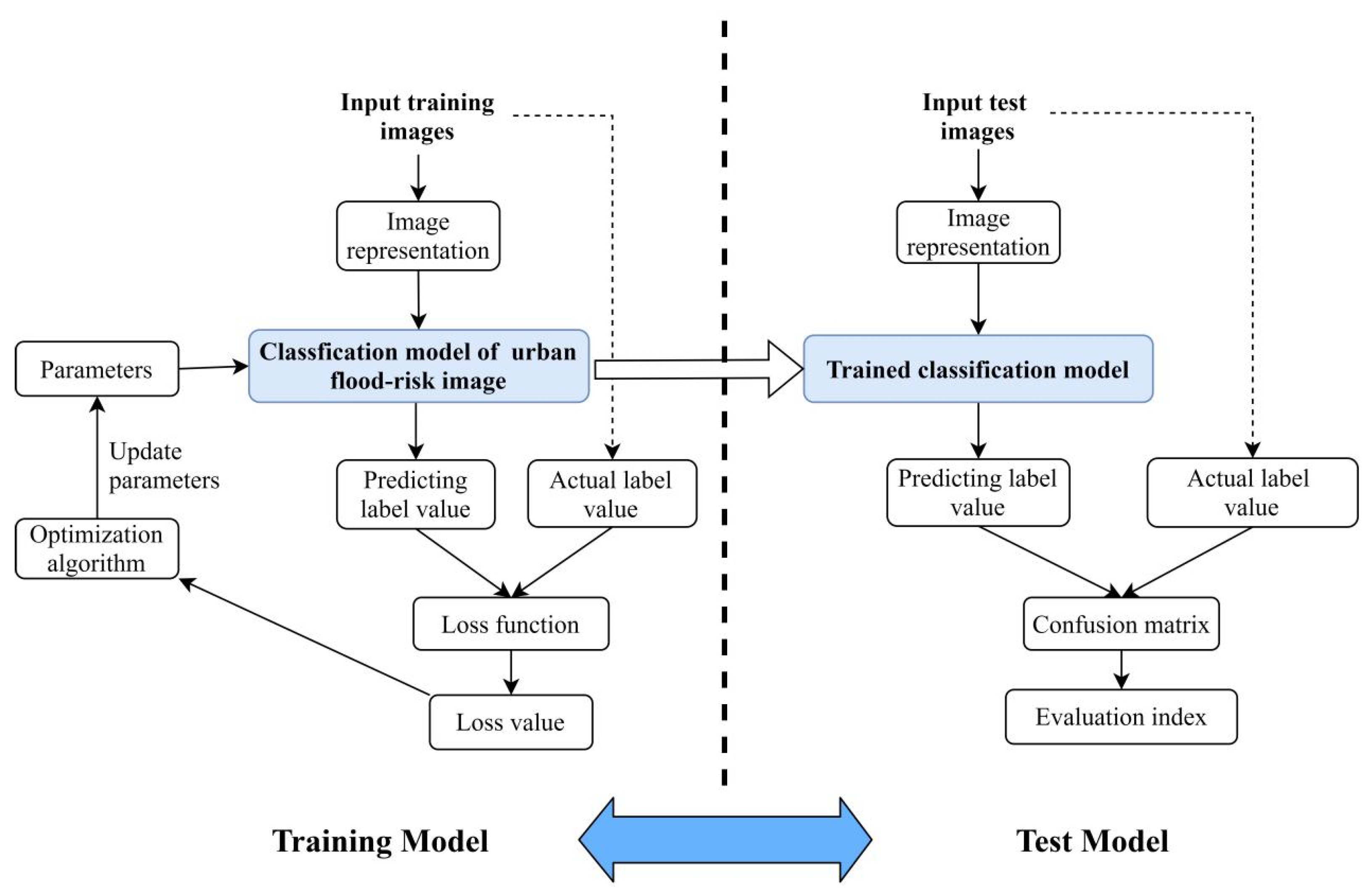
2.1.1. Classification Model based on Deep Learning
2.1.2. Models
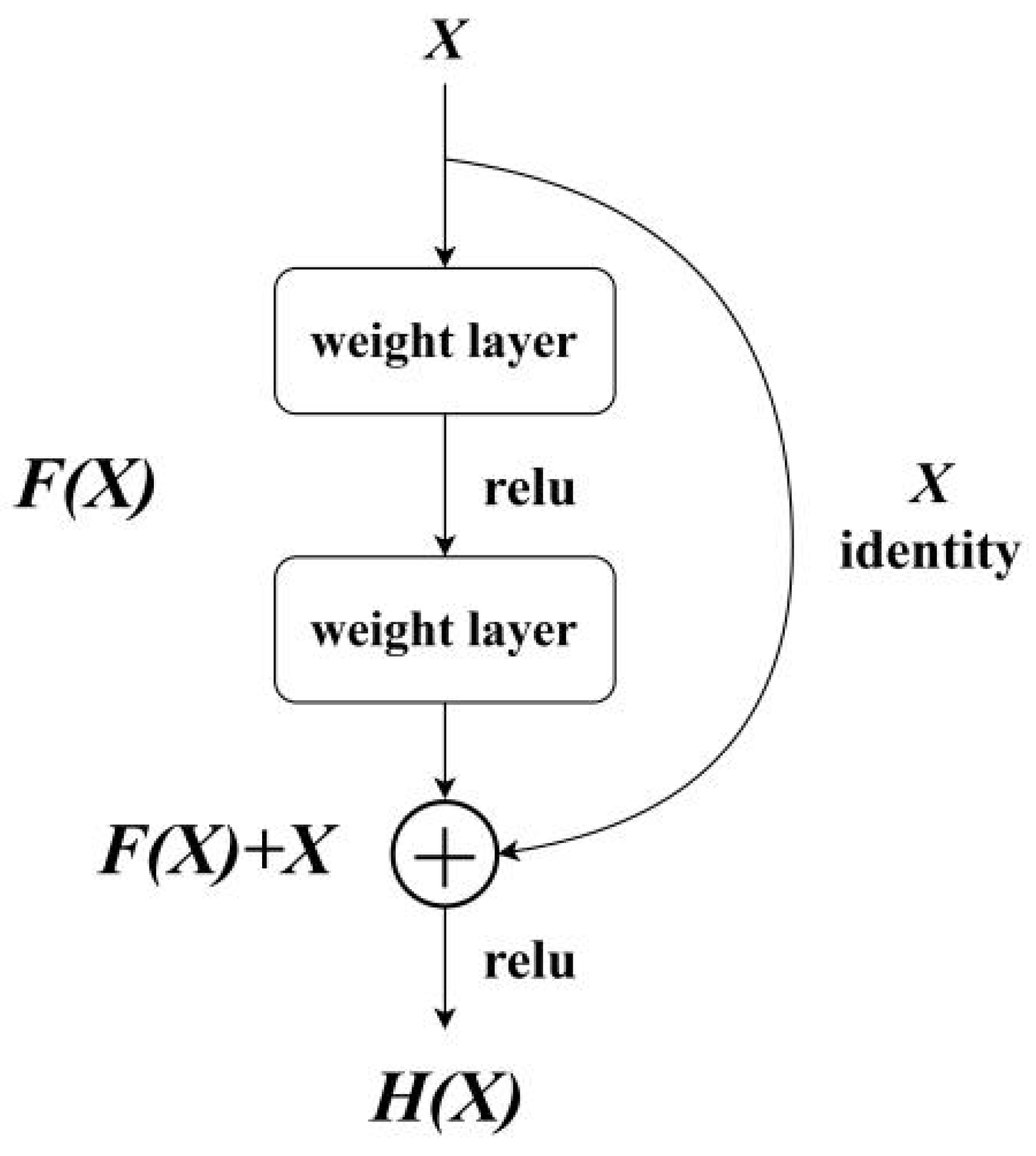
- ResNet
- 2.
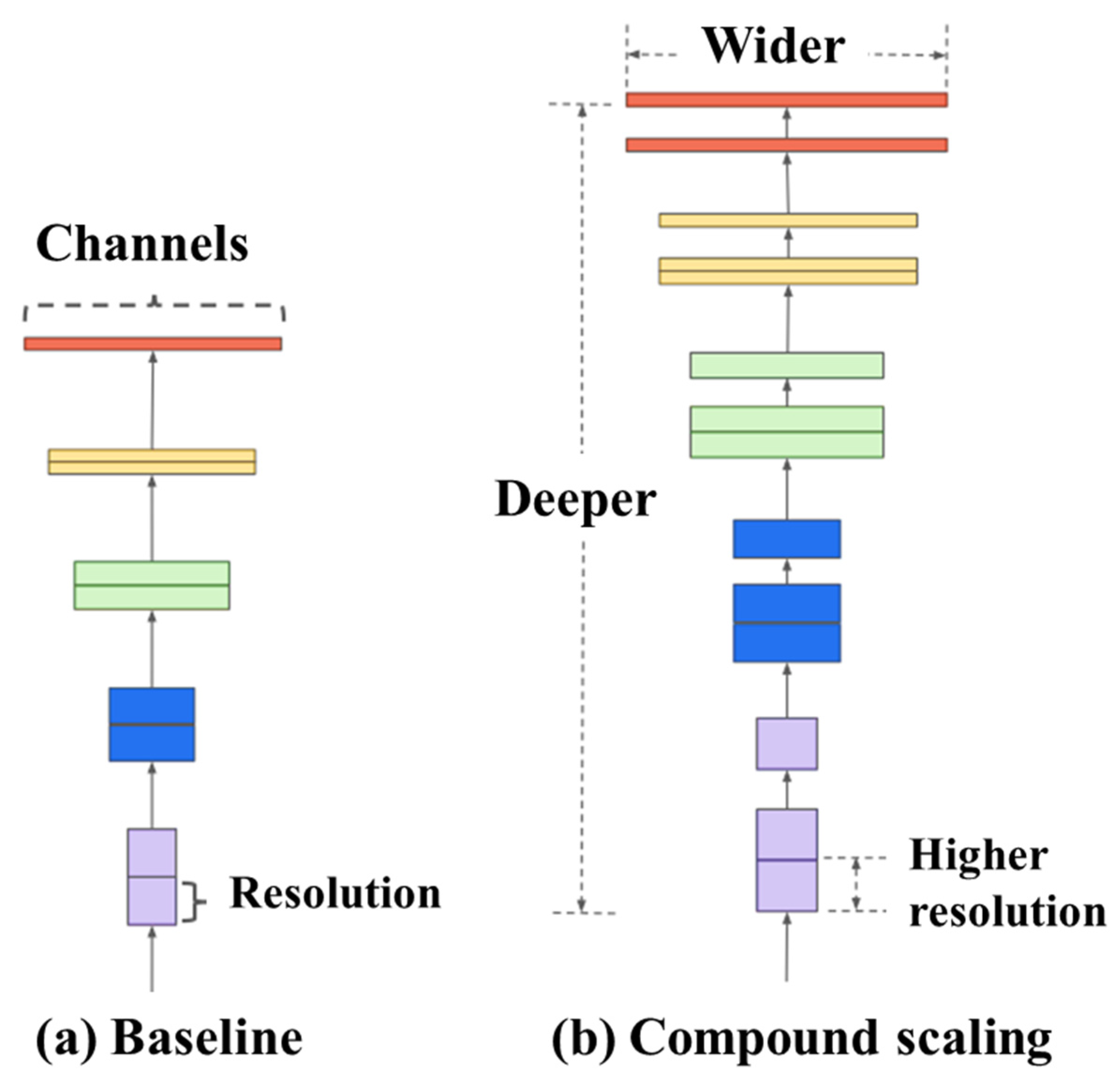
- EfficientNet
- 3.
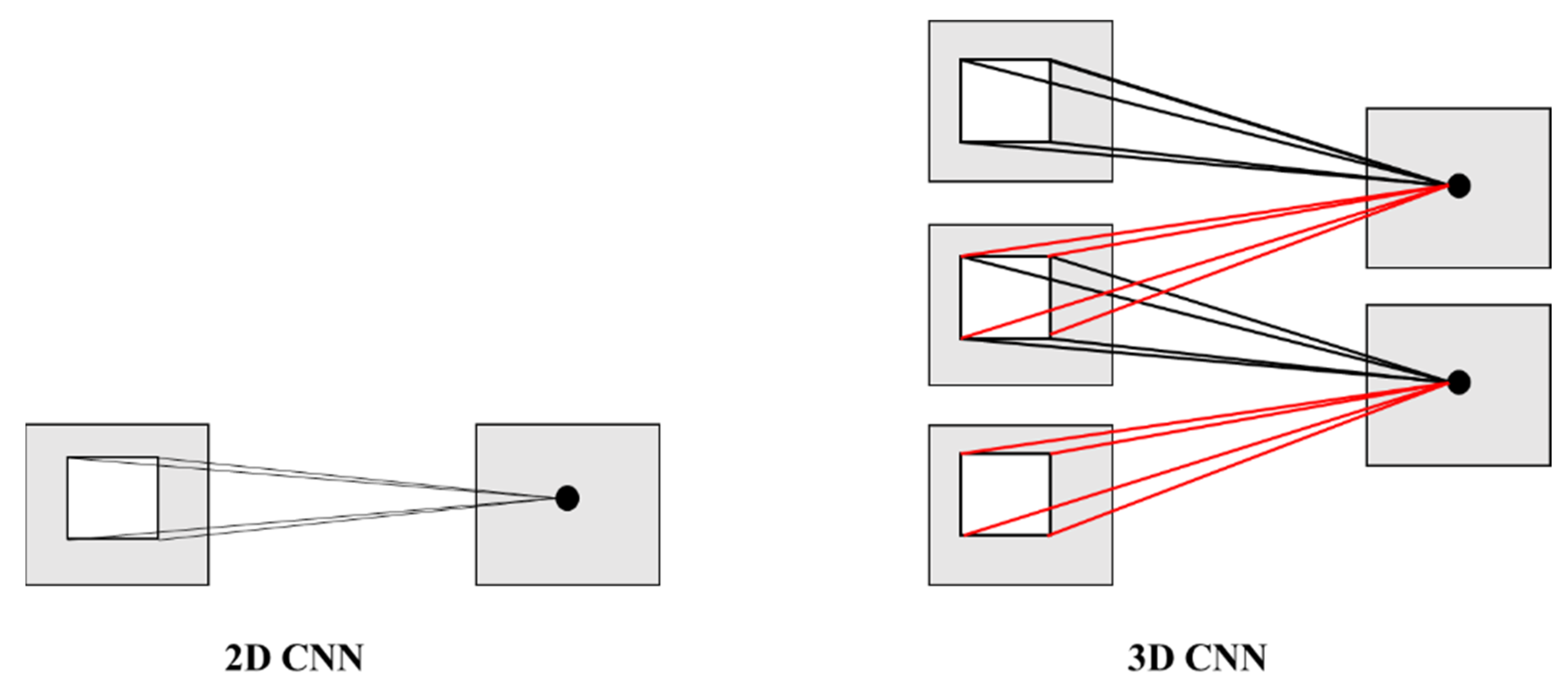
- 3D CNN
- 4.
- Other models
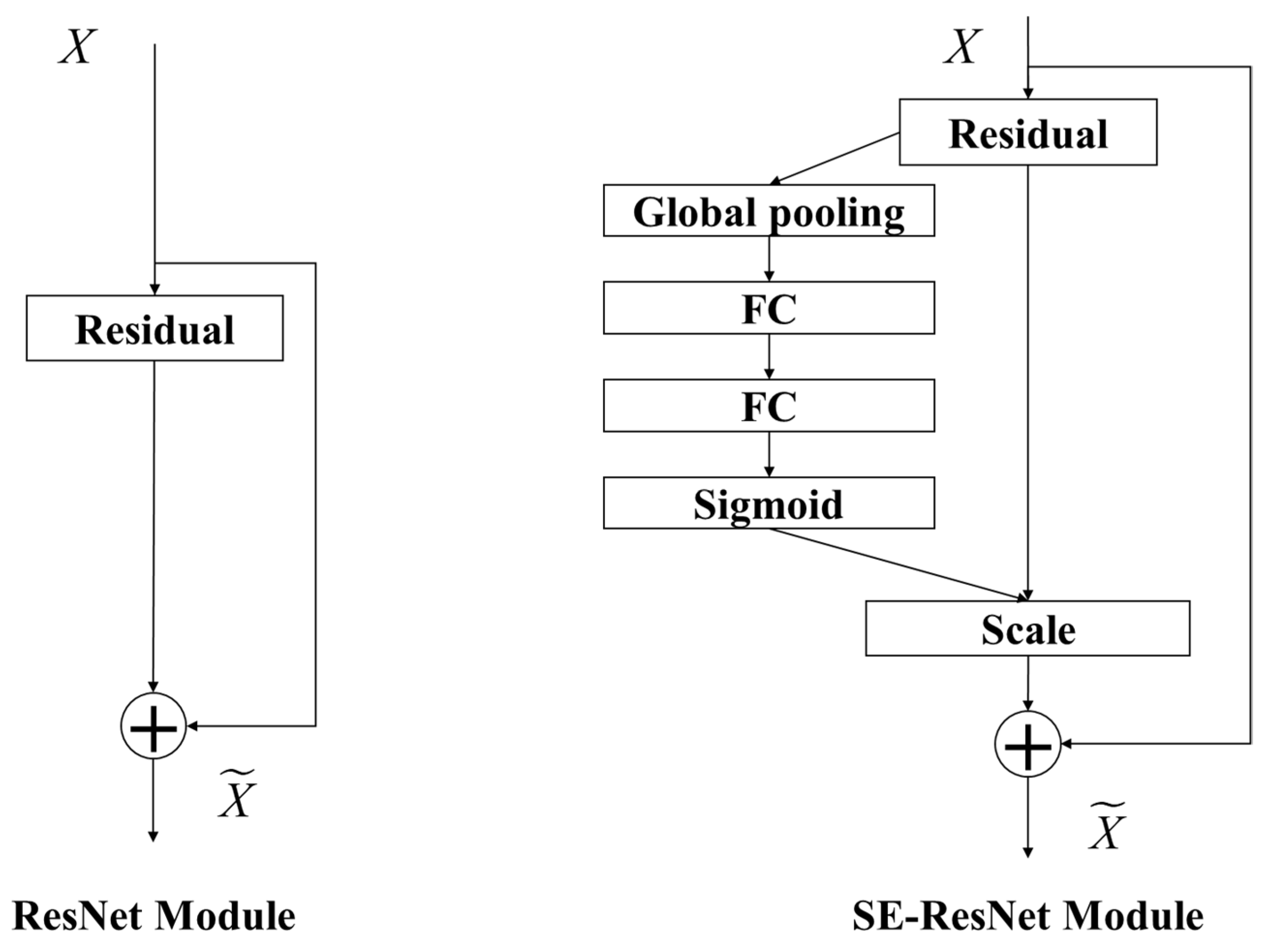
2.1.3. Attention
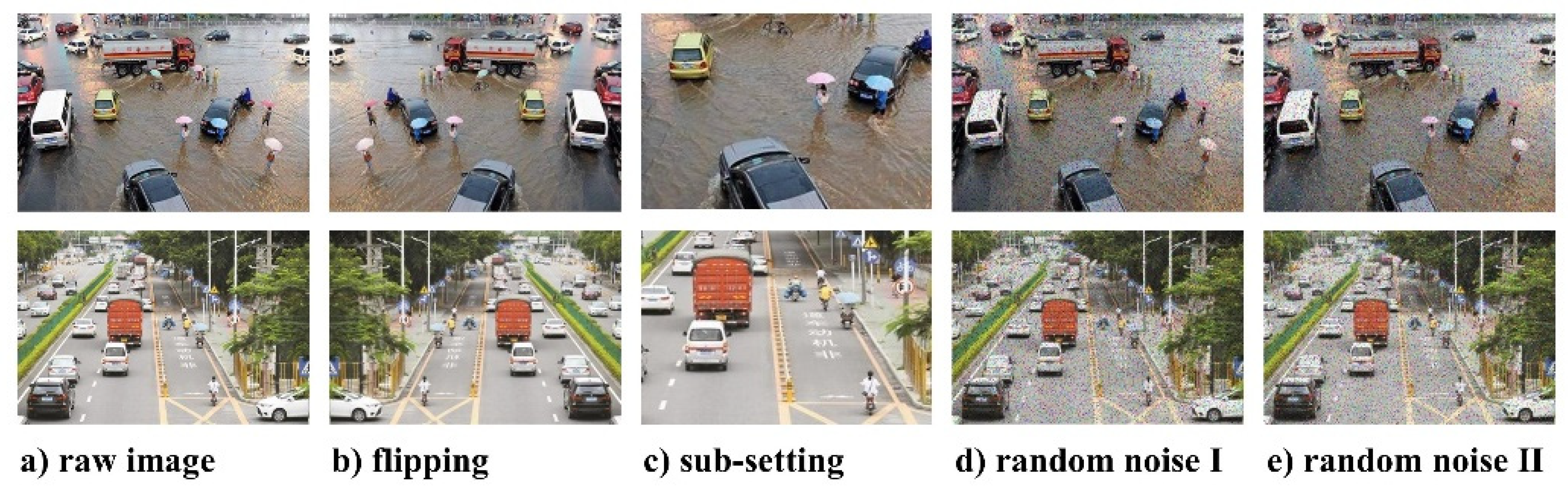
2.1.4. Data Augmentation
2.2. Threshold Method of the Time Interval Inverse Weight
3. Case Study
3.1. Case 1: Waterlogging Recognition for Public Image Data
3.2. Case 2: Waterlogging Recognition for Actual Scenarios
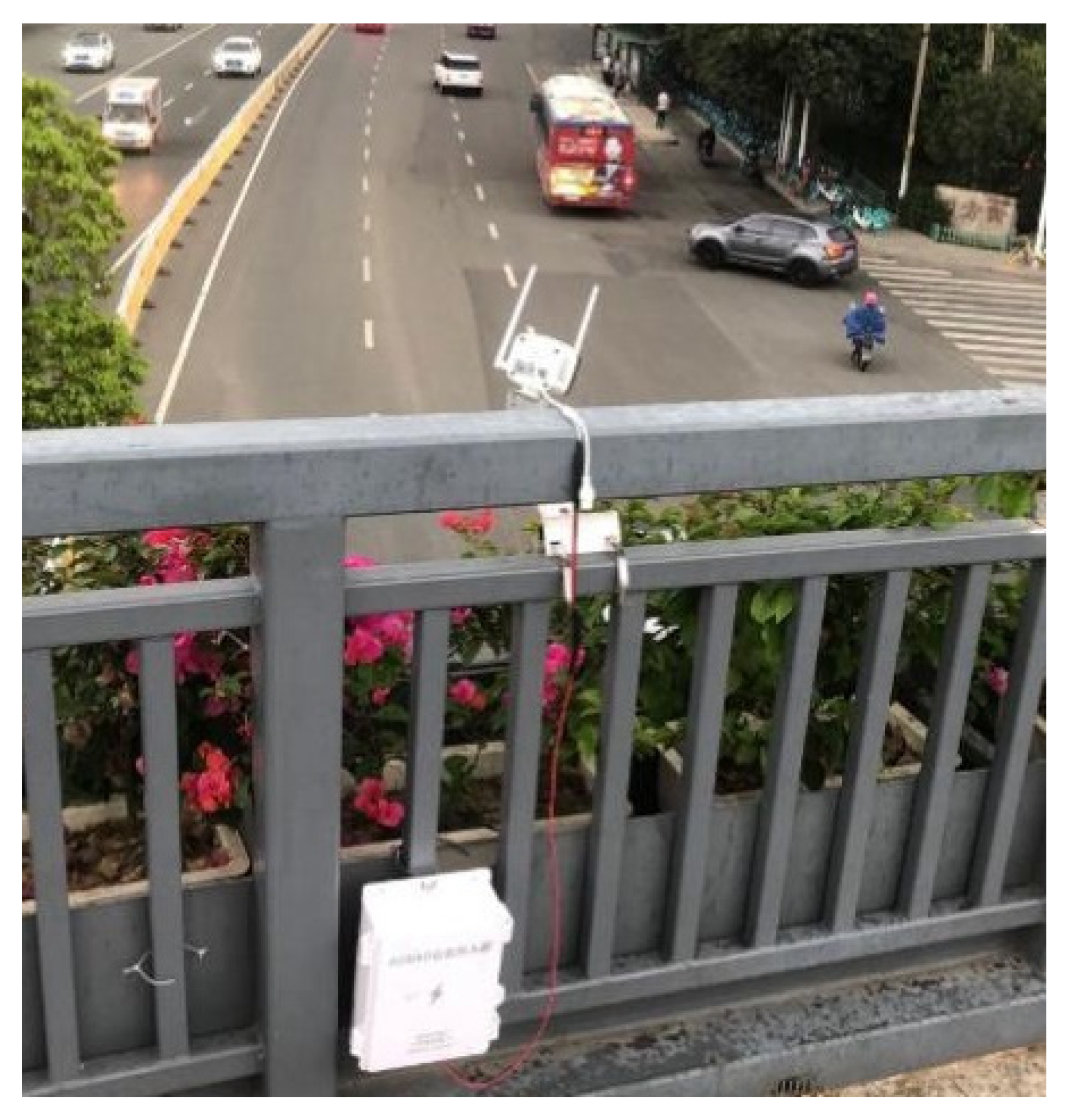
3.2.1. Experimental Setup
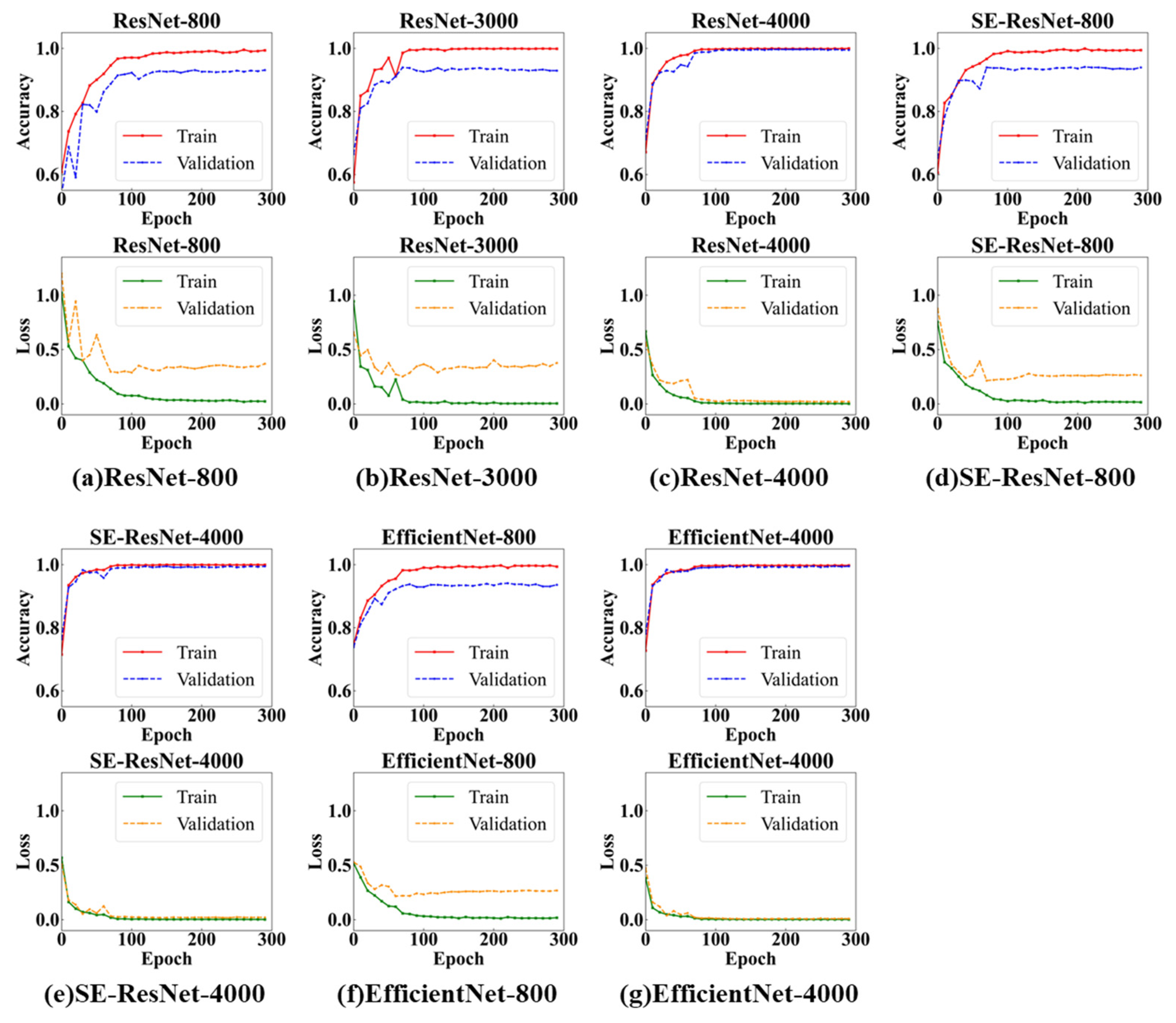
3.2.2. Training Model
4. Results and Discussion
4.1. Results of Case 1
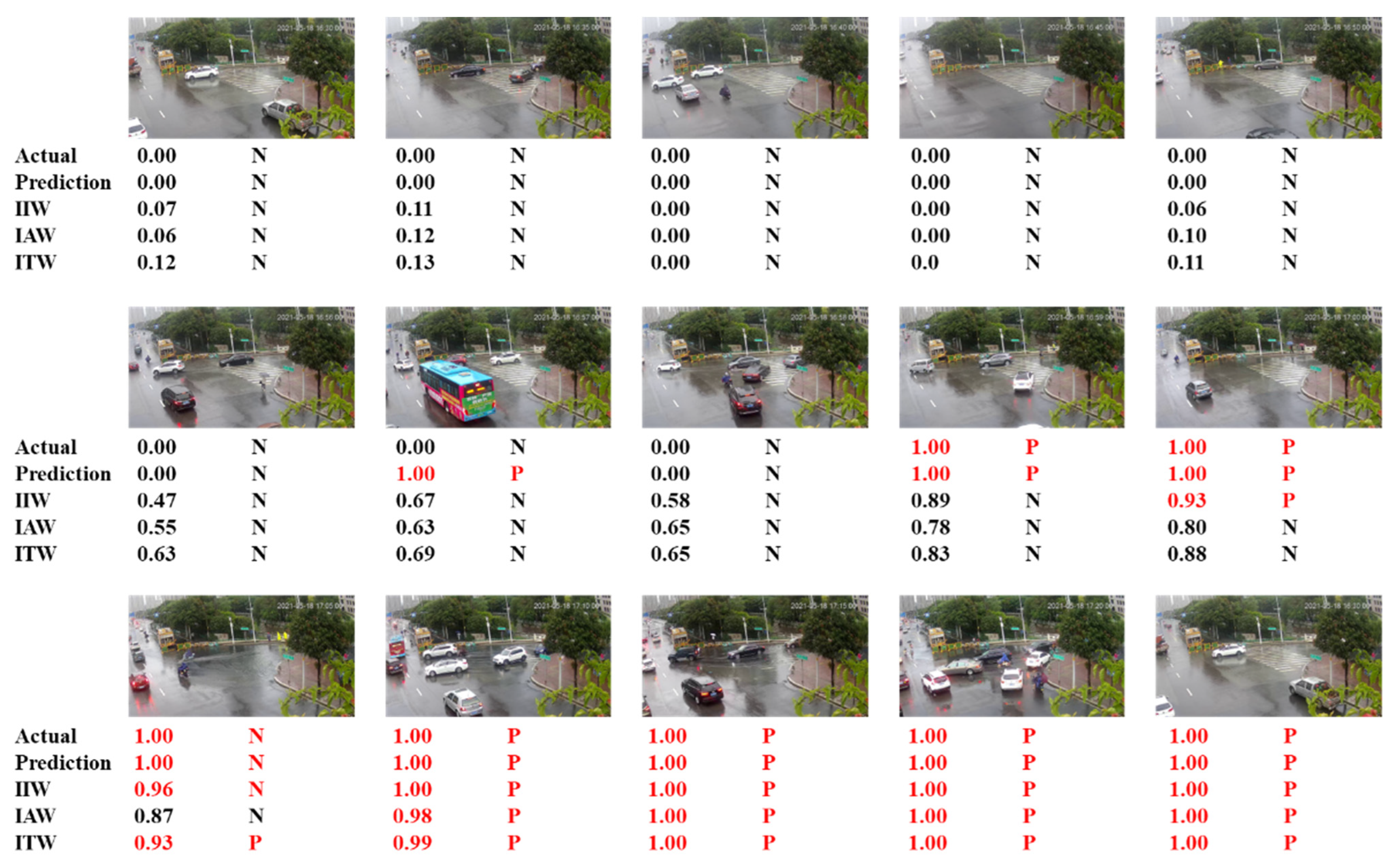
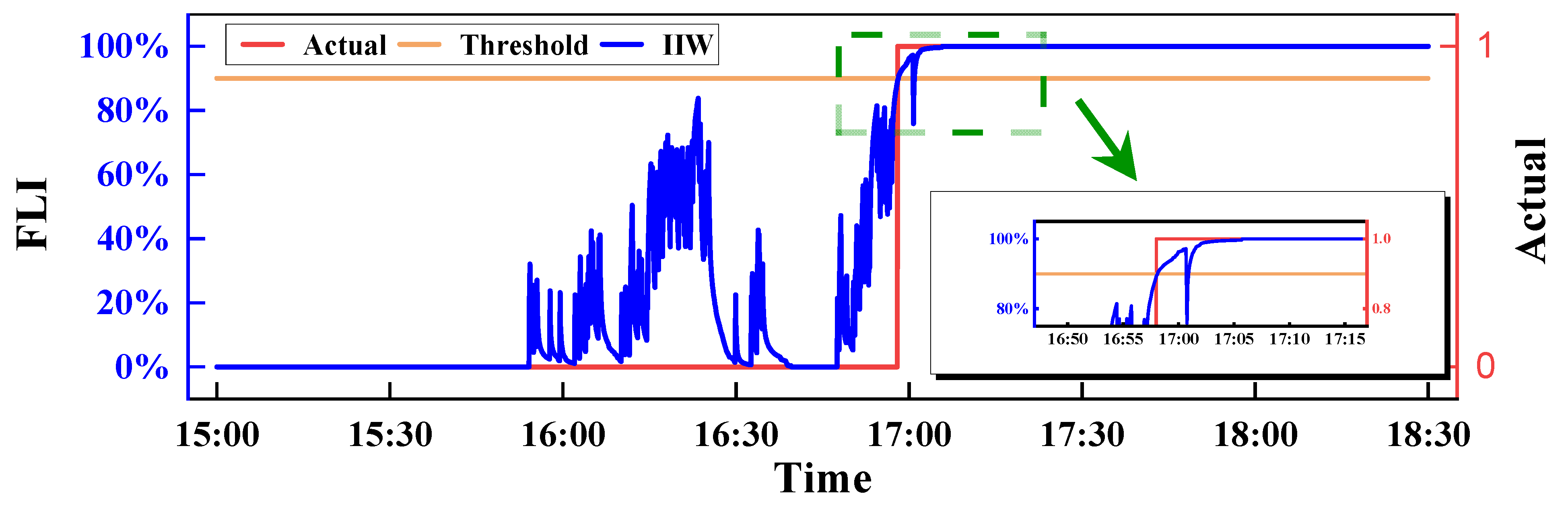
4.2. Results of Case 2
5. Conclusions
- For the task of waterlogging identification in public image datasets, data augmentation can effectively improve the model’s recognition accuracy. When the number of training datasets reaches 4000, the model’s accuracy can be stabilized to more than 99%.
- Compared with the ResNet model, the SE-ResNet model with an attention mechanism achieves higher recognition accuracy with a smaller number of training epochs.
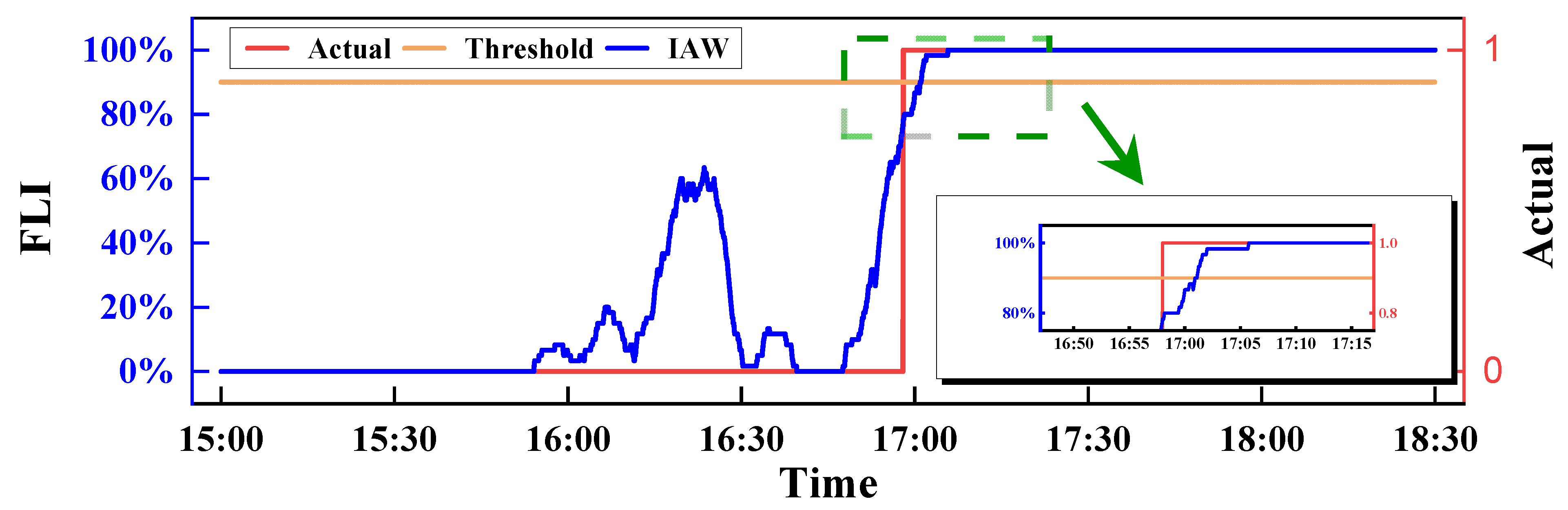
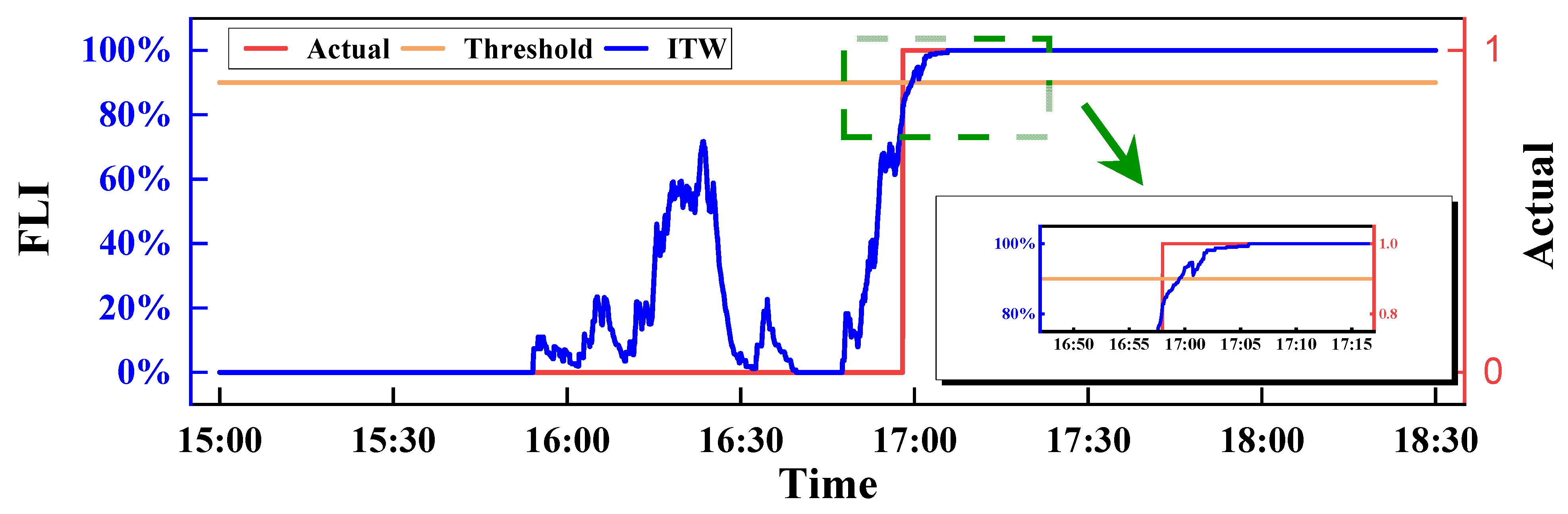
- For the actual waterlogging scene recognition task, the T-IWT method can effectively achieve waterlogging recognition. Among the flood-likelihood-index definition methods, the inverse average weight (IAW) method and the inverse time-step weight (ITW) method can achieve stable identification, with a model identification response time control falling within 30 s.
Author Contributions
Funding
Data Availability Statement
Conflicts of Interest
References
- LeCun, Y.; Kavukcuoglu, K.; Farabet, C. Convolutional Networks and Applications in Vision. In Proceedings of the 2010 IEEE International Symposium on Circuits and Systems, Paris, France, 30 May–2 June 2010; IEEE: Piscataway, NJ, USA, 2010; pp. 253–256. [Google Scholar]
- Ronneberger, O.; Fischer, P.; Brox, T. U-net: Convolutional networks for biomedical image segmentation. In Proceedings of the Medical Image Computing and Computer-Assisted Intervention–MICCAI 2015: 18th International Conference, Munich, Germany, 5–9 October 2015; pp. 234–241. [Google Scholar]
- Goecks, J.; Jalili, V.; Heiser, L.M.; Gray, J.W. Perspective How Machine Learning Will Transform Biomedicine. Cell 2020, 181, 92–101. [Google Scholar] [CrossRef]
- Galan, E.A.; Zhao, H.; Wang, X.; Dai, Q.; Huck, W.T.S. Review Intelligent Microfluidics: The Convergence of Machine Learning and Microfluidics in Materials Science and Biomedicine. Matter 2020, 3, 1893–1922. [Google Scholar] [CrossRef]
- Litjens, G.; Kooi, T.; Bejnordi, B.E.; Setio, A.A.A.; Ciompi, F.; Ghafoorian, M.; van der Laak, J.A.W.M.; van Ginneken, B.; Sánchez, C.I. A survey on deep learning in medical image analysis. Med. Image Anal. 2017, 42, 60–88. [Google Scholar] [CrossRef] [PubMed] [Green Version]
- Boloor, A.; Garimella, K.; He, X.; Gill, C.; Vorobeychik, Y.; Zhang, X. Attacking vision-based perception in end-to-end autonomous driving. J. Syst. Archit. 2020, 110, 101766. [Google Scholar] [CrossRef] [Green Version]
- Khan, M.A.; El Sayed, H.; Malik, S.; Zia, M.T.; Alkaabi, N.; Khan, J. A journey towards fully autonomous driving-fueled by a smart communication system. Veh. Commun. 2022, 36, 100476. [Google Scholar] [CrossRef]
- Cheng, J.; Zhang, L.; Chen, Q.; Hu, X.; Cai, J. A review ofvisual SLAM methods for autonomous driving vehicles. Eng. Appl. Artif. Intell. 2022, 114, 104992. [Google Scholar] [CrossRef]
- Su, Y.; Shan, S.; Chen, X.; Gao, W. Face Recognition: A Literature Survey. IEEE Trans. Image Process. 2009, 18, 1885–1896. [Google Scholar] [CrossRef]
- Santra, B.; Mukherjee, D.P. A comprehensive survey on computer vision based approaches for automatic identification of products in retail store. Image Vis. Comput. 2019, 86, 45–63. [Google Scholar] [CrossRef]
- Zhang, F.; Fu, L.S. Application of Computer Vision Technology in Agricultural Field. Prog. Mechatron. Inf. Technol. PTS 1 2 2014, 462–463, 72–76. [Google Scholar] [CrossRef]
- Ardakani, A.A.; Kanafi, A.R.; Acharya, U.R.; Khadem, N.; Mohammadi, A. Application of deep learning technique to manage COVID-19 in routine clinical practice using CT images: Results of 10 convolutional neural networks. Comput. Biol. Med. 2020, 121, 103795. [Google Scholar] [CrossRef]
- Minaee, S.; Kafieh, R.; Sonka, M.; Yazdani, S.; Jamalipour Soufi, G. Deep-COVID: Predicting COVID-19 from chest X-ray images using deep transfer learning. Med. Image Anal. 2020, 65, 101794. [Google Scholar] [CrossRef] [PubMed]
- Zhang, W.; Tang, P.; Zhao, L. Remote sensing image scene classification using CNN-CapsNet. Remote Sens. 2019, 11, 494. [Google Scholar] [CrossRef] [Green Version]
- Helber, P.; Bischke, B.; Dengel, A.; Borth, D. Eurosat: A novel dataset and deep learning benchmark for land use and land cover classification. IEEE J. Sel. Top. Appl. Earth Obs. Remote Sens. 2019, 12, 2217–2226. [Google Scholar] [CrossRef] [Green Version]
- Cao, C.; Dragicevic, S.; Li, S. Land-Use Change Detection with Convolutional Neural Network Methods. Environments 2019, 6, 25. [Google Scholar] [CrossRef] [Green Version]
- Naushad, R.; Kaur, T.; Ghaderpour, E. Deep Transfer Learning for Land Use and Land Cover Classification: A Comparative Study. Sensors 2021, 21, 8083. [Google Scholar] [CrossRef] [PubMed]
- Rahnemoonfar, M.; Murphy, R.; Miquel, M.V.; Dobbs, D.; Adams, A. Flooded area detection from UAV images based on densely connected recurrent neural networks. In Proceedings of the IGARSS 2018—2018 IEEE International Geoscience and Remote Sensing Symposium, Valencia, Spain, 22–27 July 2018; pp. 1788–1791. [Google Scholar] [CrossRef]
- Lopez-Fuentes, L.; Rossi, C.; Skinnemoen, H. River segmentation for flood monitoring. In Proceedings of the 2017 IEEE International Conference on Big Data (Big Data), Boston, MA, USA, 1–14 December 2017; pp. 3746–3749. [Google Scholar] [CrossRef] [Green Version]
- Lo, S.W.; Wu, J.H.; Lin, F.P.; Hsu, C.H. Visual sensing for urban flood monitoring. Sensors 2015, 15, 20006–20029. [Google Scholar] [CrossRef] [Green Version]
- de Vitry, M.M.; Dicht, S.; Leitão, J.P. FloodX: Urban flash flood experiments monitored with conventional and alternative sensors. Earth Syst. Sci. Data 2017, 9, 657–666. [Google Scholar] [CrossRef] [Green Version]
- Dhaya, R.; Kanthavel, R. Video Surveillance-Based Urban Flood Monitoring System Using a Convolutional Neural Network. Intell. Autom. Soft Comput. 2022, 32, 183–192. [Google Scholar] [CrossRef]
- Jiang, J.; Liu, J.; Cheng, C.; Huang, J.; Xue, A. Automatic estimation of urban waterlogging depths from video images based on ubiquitous reference objects. Remote Sens. 2019, 11, 587. [Google Scholar] [CrossRef] [Green Version]
- Li, Z.; Demir, I. U-net-based semantic classification for flood extent extraction using SAR imagery and GEE platform: A case study for 2019 central US flooding. Sci. Total Environ. 2023, 869, 161757. [Google Scholar] [CrossRef]
- Pally, R.J.; Samadi, S. Application of image processing and convolutional neural networks for flood image classification and semantic segmentation. Environ. Model. Softw. 2022, 148, 105285. [Google Scholar] [CrossRef]
- Ning, H.; Li, Z.L.; Hodgson, M.E.; Wang, C.Z. Prototyping a Social Media Flooding Photo Screening System Based on Deep Learning. ISPRS Int. J. Geo-Inf. 2020, 9, 104. [Google Scholar] [CrossRef] [Green Version]
- Long, J.; Shelhamer, E.; Darrell, T. Fully Convolutional Networks for Semantic Segmentation. In Proceedings of the IEEE Conference on Computer Vision and Pattern Recognition, Boston, MA, USA, 7–12 June 2015; pp. 3431–3440. [Google Scholar] [CrossRef] [Green Version]
- Deng, J.; Dong, W.; Socher, R.; Li, L.-J.; Li, K.; Fei-Fei, L. ImageNet: A Large-Scale Hierarchical Image Database. In Proceedings of the 2009 IEEE Conference on Computer Vision and Pattern Recognition, Miami, FL, USA, 20–25 June 2009; pp. 248–255. [Google Scholar] [CrossRef] [Green Version]
- Lowe, D.G. Distinctive image features from scale-invariant keypoints. Int. J. Comput. Vis. 2004, 60, 91–110. [Google Scholar] [CrossRef]
- Ren, S.Q.; He, K.M.; Girshick, R.; Sun, J. Faster R-CNN: Towards Real-Time Object Detection with Region Proposal Networks. Adv. Neural Inf. Process. Syst. 2015, 28, 91–99. [Google Scholar] [CrossRef] [Green Version]
- Sen, T.; Hasan, M.K.; Tran, M.; Yang, Y.; Hoque, M.E. Selective Search for Object Recognition. In Proceedings of the 13th IEEE International Conference on Automatic Face Gesture Recognition, (FG 2018), Xi’an, China, 15–19 May 2018; pp. 357–364. [Google Scholar] [CrossRef]
- Shi, J.B.; Malik, J. Normalized cuts and image segmentation. IEEE Trans. Pattern Anal. Mach. Intell. 2000, 22, 888–905. [Google Scholar] [CrossRef] [Green Version]
- Khan, A.; Sohail, A.; Zahoora, U.; Qureshi, A.S. A survey of the recent architectures of deep convolutional neural networks. Artif. Intell. Rev. 2020, 53, 5455–5516. [Google Scholar] [CrossRef] [Green Version]
- Andrew, H.; Mark, S.; Grace, C.; Liang-Chieh, C.; Bo, C.; Mingxing, T.; Weijun, W.; Yukun, Z.; Ruoming; Vijay, V. Searching for mobilenetv3. In Proceedings of the IEEE/CVF International Conference on Computer Vision (ICCV), Seoul, Korea, 27 October–2 November 2019; pp. 1314–1324. [Google Scholar]
- Zhang, X.; Zhou, X.; Lin, M.; Sun, J. ShuffleNet: An Extremely Efficient Convolutional Neural Network for Mobile Devices. In Proceedings of the 2018 IEEE/CVF Conference on Computer Vision and Pattern Recognition Workshops, Salt Lake City, UT, USA, 18–22 June 2018; pp. 6848–6856. [Google Scholar] [CrossRef] [Green Version]
- He, K.; Zhang, X.; Ren, S.; Sun, J. Deep Residual Learning for Image Recognition. In Proceedings of the IEEE Computer Society Conference on Computer Vision and Pattern Recognition, Las Vegas, NV, USA, 27–30 June 2016; Volume 2016, pp. 770–778. [Google Scholar]
- Wang, F.; Jiang, M.; Qian, C.; Yang, S.; Li, C.; Zhang, H.; Wang, X.; Tang, X. Residual Attention Network for Image Classification. In Proceedings of the 2017 IEEE Conference on Computer Vision and Pattern Recognition (CVPR), Honolulu, HI, USA, 21–26 July 2017; pp. 6450–6458. [Google Scholar] [CrossRef] [Green Version]
- Tan, M.; Le, Q.V. EfficientNet: Rethinking model scaling for convolutional neural networks. In Proceedings of the 36th International Conference on Machine Learning (ICML), Long Beach, CA, USA, 9–15 June 2019; Volume 2019, pp. 10691–10700. [Google Scholar]
- Ji, S.; Xu, W.; Yang, M.; Yu, K. 3D Convolutional Neural Networks for Human Action Recognition. IEEE Trans. Pattern Anal. Mach. Intell. 2013, 35, 221–231. [Google Scholar] [CrossRef] [PubMed] [Green Version]
- Huang, G.; Liu, Z.; Pleiss, G.; van der Maaten Maaten, L.; Weinberger, K.Q. Convolutional Networks with Dense Connectivity. IEEE Trans. Pattern Anal. Mach. Intell. 2022, 44, 8704–8716. [Google Scholar] [CrossRef] [Green Version]
- Vaswani, A.; Shazeer, N.; Parmar, N.; Uszkoreit, J.; Jones, L.; Gomez, A.N.; Kaiser, Ł.; Polosukhin, I. Attention is all you need. Adv. Neural Inf. Process. Syst. 2017, 2017, 5999–6009. [Google Scholar]
- Shorten, C.; Khoshgoftaar, T.M. A survey on Image Data Augmentation for Deep Learning. J. Big Data 2019, 6, 1–48. [Google Scholar] [CrossRef]
- Varol, G.; Laptev, I.; Schmid, C. Long-Term Temporal Convolutions for Action Recognition. IEEE Trans. Pattern Anal. Mach. Intell. 2018, 40, 1510–1517. [Google Scholar] [CrossRef] [PubMed] [Green Version]


| Parameter | Description |
|---|---|
| S | The model judgment result (no waterlogging risk/negative is recorded as 0, and the waterlogging risk/active is recorded as 1) |
| n | The backtracking time |
| t | The time of determination |
| The weight | |
| m | The number of image frames in a unit time interval |
| The actual time of waterlogging | |
| The time of the waterlogging occurrence obtained by the threshold method of the inverse weight of the time interval |
| Highest Accuracy | Best Number of Epochs | |
|---|---|---|
| ResNet-800 | 93.46% | 286 |
| ResNet-3000 | 94.30% | 72 |
| ResNet-4000 | 99.83% | 201 |
| SE-ResNet-800 | 94.30% | 214 |
| SE-ResNet-4000 | 99.50% | 83 |
| Efficient-800 | 94.52% | 208 |
| Efficient-4000 | 99.52% | 70 |
Disclaimer/Publisher’s Note: The statements, opinions and data contained in all publications are solely those of the individual author(s) and contributor(s) and not of MDPI and/or the editor(s). MDPI and/or the editor(s) disclaim responsibility for any injury to people or property resulting from any ideas, methods, instructions or products referred to in the content. |
© 2023 by the authors. Licensee MDPI, Basel, Switzerland. This article is an open access article distributed under the terms and conditions of the Creative Commons Attribution (CC BY) license (https://creativecommons.org/licenses/by/4.0/).
Share and Cite
Huang, H.; Lei, X.; Liao, W.; Li, H.; Wang, C.; Wang, H. A Real-Time Detecting Method for Continuous Urban Flood Scenarios Based on Computer Vision on Block Scale. Remote Sens. 2023, 15, 1696. https://doi.org/10.3390/rs15061696
Huang H, Lei X, Liao W, Li H, Wang C, Wang H. A Real-Time Detecting Method for Continuous Urban Flood Scenarios Based on Computer Vision on Block Scale. Remote Sensing. 2023; 15(6):1696. https://doi.org/10.3390/rs15061696
Chicago/Turabian StyleHuang, Haocheng, Xiaohui Lei, Weihong Liao, Haichen Li, Chao Wang, and Hao Wang. 2023. "A Real-Time Detecting Method for Continuous Urban Flood Scenarios Based on Computer Vision on Block Scale" Remote Sensing 15, no. 6: 1696. https://doi.org/10.3390/rs15061696