Spatial-Spectral-Associative Contrastive Learning for Satellite Hyperspectral Image Classification with Transformers

Abstract

Albeit hyperspectral image (HSI) classification methods based on deep learning have presented high accuracy in supervised classification, these traditional methods required quite a few labeled samples for parameter optimization. When processing HSIs, however, artificially labeled samples are always insufficient, and class imbalance in limited samples is inevitable. This study proposed a Transformer-based framework of spatial–spectral–associative contrastive learning classification methods to extract both spatial and spectral features of HSIs by the self-supervised method. Firstly, the label information required for contrastive learning is generated by a spatial–spectral augmentation transform and image entropy. Then, the spatial and spectral Transformer modules are used to learn the high-level semantic features of the spatial domain and the spectral domain, respectively, from which the cross-domain features are fused by associative optimization. Finally, we design a classifier based on the Transformer. The invariant features distinguished from spatial–spectral properties are used in the classification of satellite HSIs to further extract the discriminant features between different pixels, and the class intersection over union is imported into the loss function to avoid the classification collapse caused by class imbalance. Conducting experiments on two satellite HSI datasets, this study verified the classification performance of the model. The results showed that the self-supervised contrastive learning model can extract effective features for classification, and the classification generated from this model is more accurate compared with that of the supervised deep learning model, especially in the average accuracy of the various classifications.

1. Introduction

After decades of rapid development, applications of HSIs have made remarkable progress, especially in the field of satellite hyperspectral remote sensing [1]. Various satellites, such as Earth Observing 1 (EO-1) [2], Huanjing-1A (HJ-1A) [3], Gaofen-5 (GF-5) [4], DLR Earth Sensing Imaging Spectrometer (DESIS) [5], preferred reporting items for systematic reviews and meta-analyses (PRISMA) [6], and Gaofen-14 (GF-14) [7] have been launched in recent decades, of which the spatial and spectral resolution have experienced significant improvement [7]. Compared with airborne HSIs, satellite HSIs have obvious advantages in ground applications at large scale, such as mineral exploration [4], precise agriculture [8], ecological monitoring [5], and land cover classification [9]. HSI classification is one of the core processing techniques for various applications, aiming to assign each pixel of HSI an accurate class label. However, the complex spatial–spectral structure and high-dimensional information of hyperspectral data [10] make it difficult to obtain optimal classification results by original satellite hyperspectral data without pre-processing.

In the initial stage of the HSI classification, the traditional methods mainly focused on the use of spectral features, such as spectral angle mapper (SAM) [11] and maximum-likelihood (ML) [12]. With the improvement of spatial resolution, the intra-class heterogeneity also increases [13], and it is quite difficult for the algorithms to classify accurately only by spectral features. The spatial characteristics of pixel neighborhoods can provide extra information to fix the problem. Methods such as morphological attribute profiles (MAPs) [14], extend morphological attribute profiles (EMAPs) [15], and Markov random field (MRF) [16] have been used for associative extraction of both spatial and spectral features. However, these methods are highly dependent on professional prior knowledge and the classification performance is greatly affected by hand-crafted spectral–spatial features, making the model generalization ability relatively weak [17].

With the continuous development of deep learning, it has also received extensive attention in hyperspectral image classification tasks. This is attributed to its obvious advantages in mining feature representations that are conducive to HSI classification from the data itself, and thus, deep learning seldom relies on data prior information or professional knowledge. As a typical data-driven method, deep learning, such as stacked autoencoder (SAE) [18] and deep belief network (DBN) [19], usually uses principal component analysis (PCA) to reduce the dimension of HSI data to several bands. Hence, researchers have begun to develop more flexible deep models for HSI classifications. Among them, convolutional neural networks (CNN) have achieved state-of-the-art performance [20,21]; the one-dimensional convolutional neural network (1D-CNN) [22] inputs each pixel as a vector in the spectral domain into the model to extract effective spectral features for hyperspectral image classification, while lacking the full use of spatial information. The classification method based on a two-dimensional convolutional neural network (2D-CNN) [23] performs better with a smoother visual effect compared with that from the 1D-CNN method. However, there are still defects of 2D-CNN in retaining the spatial–spectral structure information of HSIs, and the ability to capture context information is weak. The classification method based on a three-dimensional convolutional neural network (3D-CNN) [22] combines 1D-CNN and 2D-CNN to extract the spatial–spectral features of HSIs in a unified framework. Not only is the network structure simpler and more flexible, but also the classification effect is more obvious.

However, the performance of convolutional neural networks is determined by the size of the convolution kernel and the number of convolution channels, which results in a great limitation on the receptive field of the CNN model and the large difficulty in capturing long-range dependencies similar to spectral sequences [24]. The Transformer [25], which is developed in the field of natural language processing (NLP), has attracted rising attention due to its superior performance compared with convolutional neural networks [26]. The application effect of the Transformer in the hyperspectral image classification task is also encouraging. Previously published research used the Transformer module for hyperspectral image classification, and some combined CNN for hyperspectral image classification. He et al. [27] combined CNN with Transformer and used CNN and Transformer to extract spatial and spectral features, respectively. Qing et al. [28] designed different Transformers for spatial and spectral features, and captured the long-range dependencies information through a self-attention mechanism. Yang et al. [29] embedded CNN into the Transformer to extract detailed spectral features and local spatial information using CNN. Zou et al. [30] proposed a local-enhanced spectral–spatial transformer (LESSFormer), which extracts the underlying features through CNN and forms feature patches, and further extracts local and global spatial-spectral features through Transformer, significantly improving classification performance. Tu et al. [31] improved the way the original HSI features are embedded, allowing the Transformer module to more efficiently capture long-range dependencies between multi-scale features through local semantic feature aggregation.

The above deep learning methods are all trained in a supervised manner, and the classification performance is determined by the number and quality of labeled samples [32]. For satellite hyperspectral images, the cost of obtaining large amounts of labeled samples is too high to afford. Moreover, there are usually problems involved in class imbalance in the limited labeled samples, which greatly limits the practical application in satellite hyperspectral image classification. Self-supervised learning [33,34] has been widely used in the field of computer vision, with an obvious advantage that the training hardly relies on labeled samples. Therefore, studies on self-supervised learning have been well documented in HSI classification. Wang et al. [35] conducted concatenate contrastive learning at sub-pixel, pixel, and super-pixel levels based on multi-scale features in the spatial domain. Zhu et al. [36] also used multi-scale patches in the spatial domain as learning objects and put efficient asymmetric dilated convolution (EADC) into the contrastive learning framework to realize the learning of consistent features in the neighborhood of the target pixel. While ensuring accuracy, the computational efficiency has been improved. Some works constructed multi-views of the same scene through PCA [37,38]. After a certain augmented transformation, they used a contrastive learning framework for consistent feature learning. It can be seen that the self-supervised learning strategy based on contrastive learning has achieved good research results in hyperspectral image classification tasks. Guan et al. [39] considered both spectral and spatial information and found shared information between the spatial domain and spectral domain through a contrastive learning framework to extract high-level semantic information that is helpful for classification. Hu et al. [40] introduced Transformer into the bootstrap your own latent (BYOL) framework to replace 2D-CNN for feature extraction, but the model reshaped the original data into a one-dimensional sequence, which destroyed the spatial dependence in the two-dimensional space.

The self-supervised learning strategy based on contrastive learning has achieved good research results in hyperspectral image classification tasks. However, under practical application scenarios such as satellite hyperspectral image classification, there are still the following problems to be solved. First of all, although the use of PCA to generate spatial multi-views can reduce the redundant information between various bands [37], the spatial contrastive learning on the same principal component has difficulty in augmenting the diversity of samples. More importantly, there is an obvious lack of mining of spectral feature similarity of hyperspectral data, which will reduce the robustness of the model [41]. Secondly, the previous algorithms have shown that classifiers using only spatial features or spectral features will limit the improvement of classification performance. The combination of spatial and spectral features is the mainstream practice of feature extraction in supervised hyperspectral image classification. However, under the self-supervised framework, it is difficult to process cross-domain information. Finally, in satellite hyperspectral images, the distribution of ground objects is often uneven, leading to the widespread problem of class imbalance. Classifiers need to adapt the characteristics of satellite hyperspectral images.

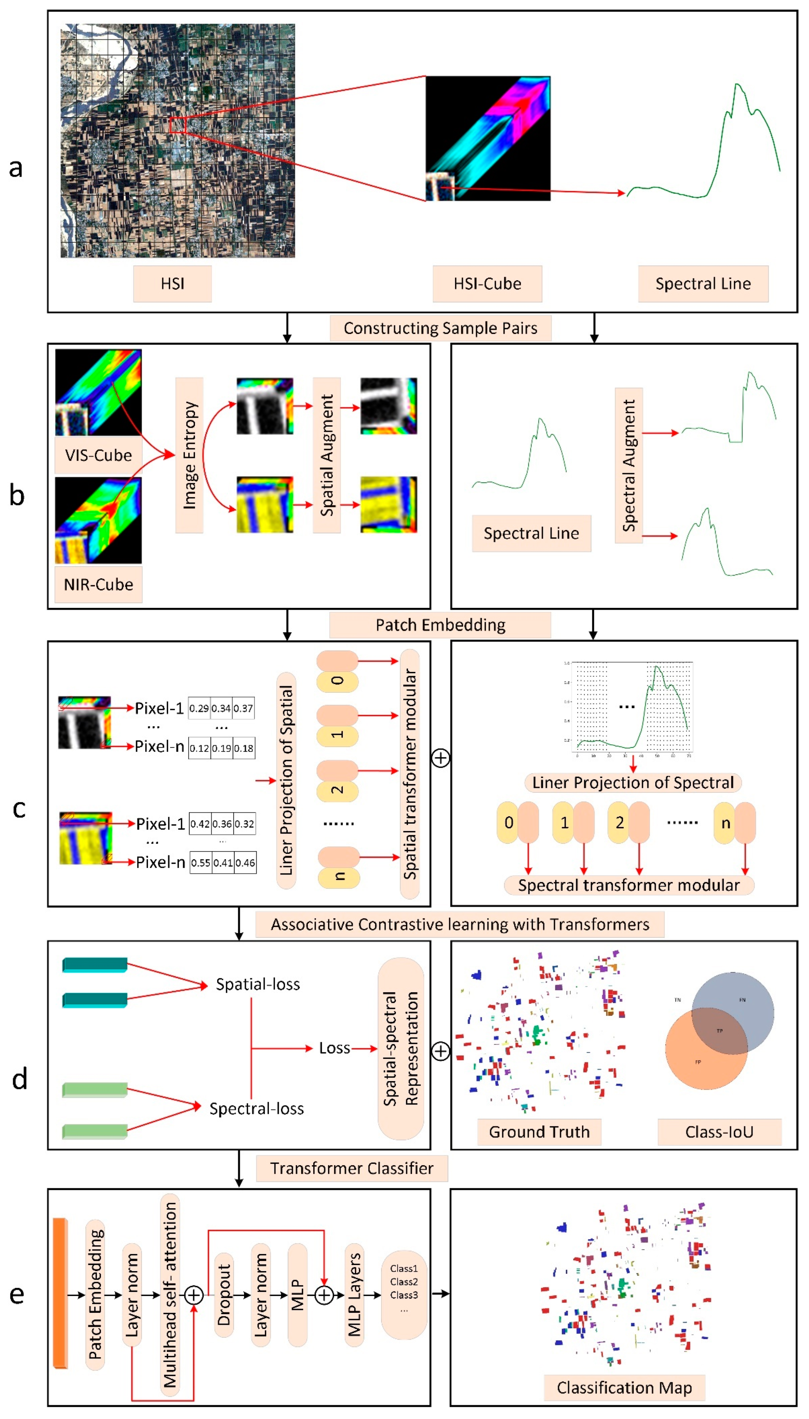
To solve the above problems, we propose a satellite hyperspectral image classification method based on spatial–spectral associative contrastive learning (SSACT), which is completely based on the Transformer network. The biggest highlight of SSACT is that it can capture the long-range dependence of temporal sequence data, which significantly enhances the ability in extracting spectral detail features and spatial dependence of hyperspectral data. SSACT performs both spatial and spectral invariant features of hyperspectral data in a self-supervised manner under a unified contrastive learning framework, and further realizes feature fusion by associative training. SSACT develops a classifier based on the contrastive learning Transformer framework to learn the fusion features and complete the hyperspectral image classification. Our main contributions are as follows:

• The study innovatively builds the Transformer-based associative contrastive learning framework for satellite hyperspectral image classification, which helps to learn the unique features of the spatial domain and spectral domain simultaneously, and improves the feature representation ability and classification performance of the model;
• We introduce the image entropy module to extract certain bands with rich spatial information and increase the diversity of spatial domain samples, which improves the robustness of spatial contrastive learning;
• The pixels in the spatial domain and the blocks in the spectral domain are added as the learning embedding units of the Transformer, respectively. The multi-head attention mechanism of the Transformer is used to extract the spatial dependence and spectral detail features of the target pixel, which is beneficial to the fusion expression of spatial–spectral features;
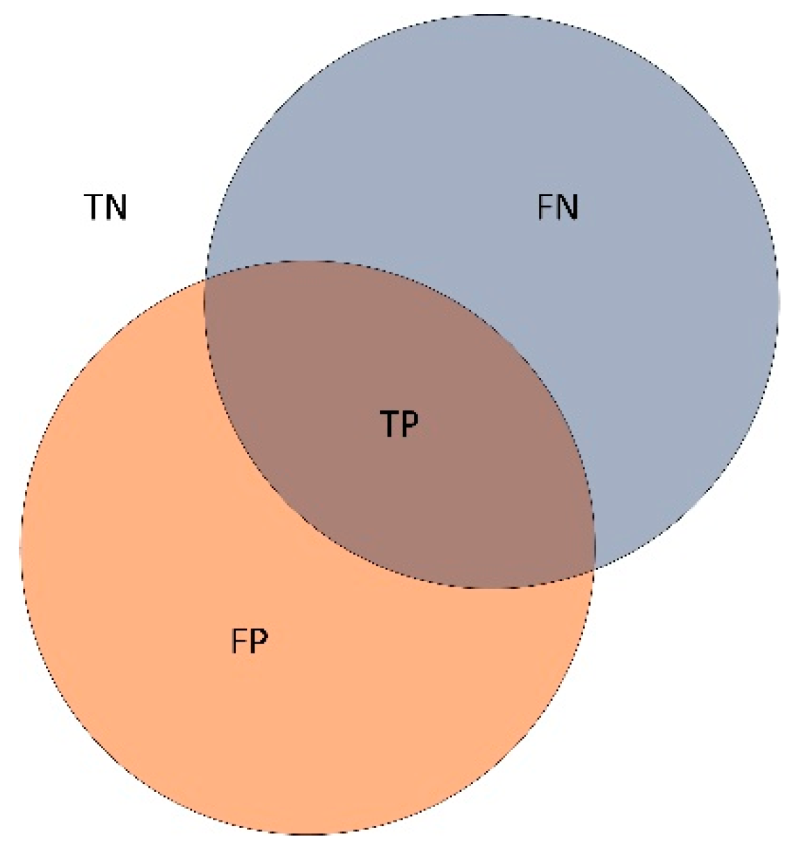
• We introduce the class intersection over union into the classification loss function, which effectively diminishes the inter-class classification difference caused by the class imbalance of samples. The effectiveness of the algorithm is proved by the satellite hyperspectral image classification experiments.

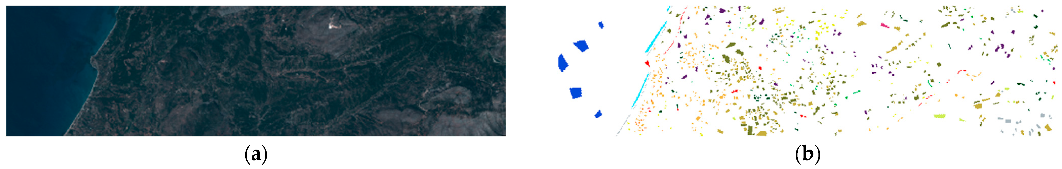
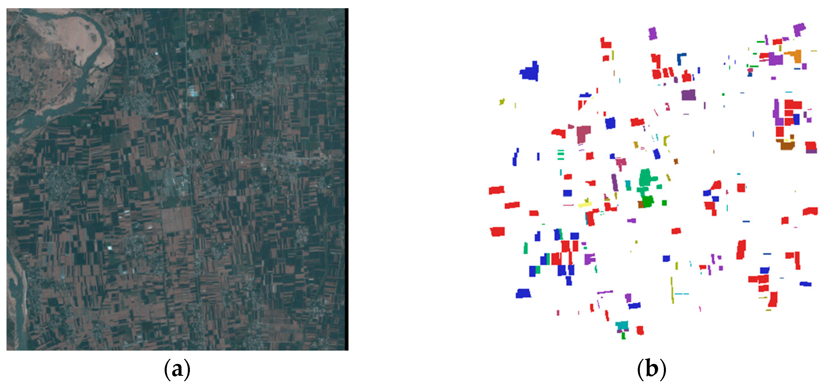
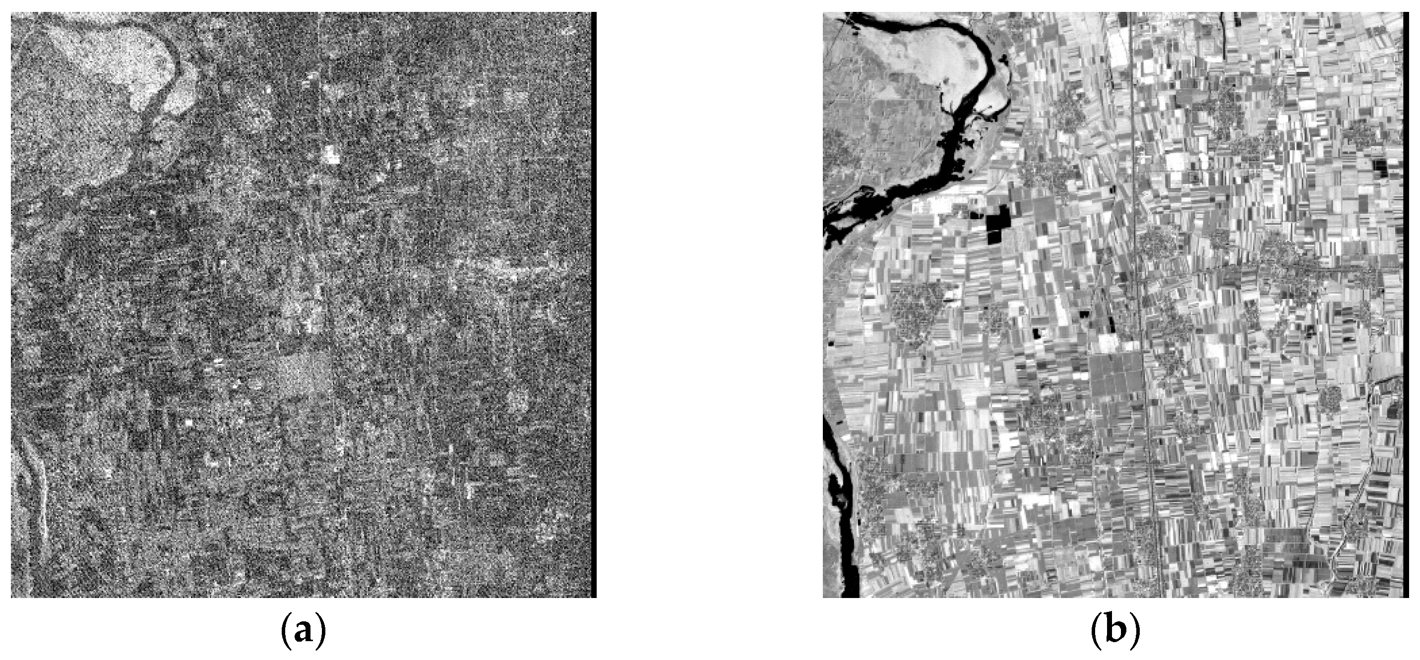
The remaining part of the paper proceeds as follows. Section 2 introduces the experimental datasets, which include two real satellite HSI datasets, and describes the proposed spatial–spectral–associative contrastive learning with Transformers for satellite hyperspectral image classification. Section 3 analyzes the experimental results of the proposed method and the compared methods. Conclusions are summarized in Section 4.

2. Materials and Methods

2.1. Datasets

To verify the effectiveness of the algorithm model, we selected two satellite hyperspectral image datasets, including HyRANK Loukia, and GF14 hyperspectral image datasets. The ground truth object classes of the two datasets, as well as the resolution and spectral range, are different, which is conducive to evaluating the generalization performance of the classification algorithm. In the contrastive learning stage, only the original data is input, without any labeled sample information. In the classification process, to restore the problem of class imbalance as much as possible, 10% of the labeled samples are selected for training in equal proportion for each class. From the number of training samples of the two data sets, as shown in

Table 1. Land cover classes with samples number for the HL dataset.

Class	Land Cover Types	Train Number	Test Number
1	Dense Urban Fabric	29	288
2	Mineral Extraction Sites	7	67
3	Non-Irrigated Arable Land	54	542
4	Fruit Trees	8	79
5	Olive Groves	140	1401
6	Broad-Leaved Forest	22	223
7	Coniferous Forest	50	500
8	Mixed Forest	107	1072
9	Dense Sclerophyllous Vegetation	379	3793
10	Sparce Sclerophyllous Vegetation	280	2803
11	Sparsely Vegetated Areas	40	404
11	Rocks and Sand	49	487
13	Water	139	1393
14	Coastal Water	45	451
Total		1349	13,503

and

Table 2. Land cover classes with samples number for the GF14 dataset.

Class	Land Cover Types	Train Number	Test Number
1	Cabbage	130	1300
2	Potato	1270	12,695
3	Green Chinese Onion	67	673
4	Wheat	4583	45,826
5	Cole Flowers	40	403
6	Corn	251	2506
7	Chinese Cabbage	171	1708
8	Peanut	2126	21,258
9	Broad Bean	15	145
10	Pepper	180	1796
11	Pit Pond	298	2981
11	Greenhouse	650	6500
13	Poplar Tree	216	2157
14	Peach	272	2719
15	Privet Tree	506	5064
16	Maple	100	1001
17	Pear Tree	278	2776
18	Cherry Plum	200	1997
Total		11,353	113,505

, the ratio between the maximum number of samples and the minimum number of samples is 56.61 and 316.04, respectively. The class imbalance is very serious, especially in GF14 hyperspectral image datasets, which reflects the messy distribution of ground truth. The data value was normalized to the range from 0 to 1. The datasets are described as follows:

The first dataset was the HyRANK Loukia satellite hyperspectral dataset (HL) [42], photographed by the Hyperion sensor. The number of original image bands is 242, the spatial resolution is 30 m, and the spatial size is 250 $\times$ 1376. However, due to the same reasons as IP dataset, this dataset contains only 176 bands. The sample information provided by the dataset indicates that the image mainly contains 16 land cover types. The class information and the number of training and test samples are shown in Table 1, and the false color image and sample distribution are shown in Figure 1.

The second dataset was the GF-14 satellite hyperspectral dataset (GF14) [7], photographed by the GF-14 satellite in Hubei, China, in May 2022. The number of original image bands is 70, the spatial resolution is 5 m, and the spatial size is 1240 $\times$ 1240, with 18 land cover types. The class information and the number of training and test samples are shown in Table 2, and the false color image and sample distribution are shown in Figure 2.

2.2. Workflow of the Proposed Method

In this article, we innovatively propose a spatial–spectral associative contrastive learning hyperspectral image classification framework SSACT based on Transformer, which learns the characteristics of hyperspectral data in a self-supervised way. At the same time, we introduce the class intersection over union (Class-IoU) into the classification loss function, which effectively diminishes the inter-class classification difference caused by the class imbalance of samples. The overall flow chart of the framework is shown in Figure 3.

Before using SSACT to process the data, we cut the original hyperspectral image data into a fixed-size hyperspectral data cube. Each cube is centered on the target pixel to ensure that the data cube contains the spatial context required for classification. Then the cube is divided into visible light range and non-visible light range, and the top three bands of image information entropy are extracted respectively as the input data of the spatial contrastive learning module, and common data augmentation operations such as random crop and random flip are applied. At the same time, the spectral curve of the target pixel is extracted and data augmentation operations such as random crop, random dropout, and reverse are applied as input data for the spectral contrastive learning module. In the self-supervised contrastive learning stage, we regard a single pixel and a spectral block as a word vector and input the sequence data into the Transformer through linear projection and position coding to obtain the spatial and spectral invariant features of the target pixel at the same time. We regard the invariant features obtained by associative contrastive learning as the reconstructed pixel spectral features, so the new features are still preprocessed by spectral partitioning and input into the Transformer classifier to achieve high-precision classification of satellite hyperspectral images. Next, we will introduce the details of the algorithm implementation.

2.3. Transformer

The wide application of Transformer began in the field of NLP [25] and then showed great potential in the field of computer vision [26]. In the field of remote sensing, it also reached or even exceeded the deep learning model based on CNN [43,44,45,46,47]. As already mentioned, Transformer is more suitable for processing sequence data than CNN. Firstly, Transformer can accurately capture the long-range dependencies in sequential data. We can add position coding to the sequential data. The position-encoded feature will be used as an independent patch to participate in the subsequent processing of the self-attention module, and the self-attention module finds the dependencies between different patches through the multi-head attention mechanism. Such a process is very conducive to capturing the dependencies between spectral detail features, which is of great significance for characterizing the diagnostic spectral features of ground objects. Secondly, the Transformer architecture can still capture the interaction between them when dealing with unordered data. Note that this ability is difficult for deep learning architectures based on CNN. When extracting the spatial context of the target pixel, the neighborhood pixels do not belong to the sequence data like the spectral features. However, after position coding, the neighborhood spatial information is processed in the self-attention module in the form of a patch, while other processing is based on the position. This ability is beneficial to the capture of spatial context.

2.4. Image Entropy for HSI

Entropy is a basic concept in the field of thermodynamics and information theory. As an index, entropy can represent the order or disorder in the physical sense and also represent the predictability or uncertainty of information. In all entropy, Shannon entropy [48] is one of the most common entropies, whose expression is as follows:

$$E=-{\sum }_i{p}_i{log}_2{p}_i,$$

(1)

where $p_i$ is the probability of an event. As a metric, entropy can also be used to measure the randomness or disorder of images [49]. For gray images, $p_i$ represents the probability of a certain gray level. When $p_i\in \left[\mathrm{0,1}\right]$, entropy is a positive interval metric. Therefore, the larger the entropy value, the higher the complexity of the image, and the richer the information contained in the image. For hyperspectral images, due to the different ground reflectance, the scene information obtained by different bands is also different. For the bands with larger entropy, the scene information contained is more abundant, as shown in Figure 4.

In self-supervised learning strategies, invariant features are often learned from different augmentation views of the same image, which limits the diversity of learning representations [41]. For hyperspectral images, different bands correspond to the same view scene and should have the same spatial relationship. To increase the diversity of spatial contrastive learning sample sampling and learn more general spatial invariant features, we divide the hyperspectral data into visible light range and non-visible light range from the perspective of human vision. The first three bands with largest entropy values in the two ranges are obtained as the input of spatial contrastive learning, respectively. Obviously, the spatial contrastive learning module learning has a more general spatial dependence, as shown in Figure 3b.

2.5. Spatial-Spectral Associative Contrastive Learning

Hyperspectral data contain the rich spatial and spectral information, being widely used in various fields. In the classification task, previous algorithms have shown that classifiers using only spatial features or spectral features will limit the improvement of classification performance. Therefore, the combination of spatial and spectral features is the mainstream practice of feature extraction in hyperspectral image classification. In this paper, the expression forms of spatial and spectral features in the process of self-supervised contrastive learning are fully analyzed. The spatial and spectral features are fused and extracted using associative contrastive learning. The invariant features contained in the target pixels are learned from the spatial and spectral dimensions through the spatial contrastive learning module and the spectral contrastive learning module, respectively, as shown in Figure 3c,d.

2.5.1. Data Augmentation

Before conducting contrastive learning, data augmentation is an important part of improving the generalization performance of the model. In this paper, we use two types of data augmentation operations: spatial augmentation and spectral augmentation. Spatial augmentation operations include random cropping, random flip (horizontal or vertical), random color jitter, random grayscale, and normalization. The spectral augmentation object is the spectral sequence of the target pixel; augmentation operations include random cropping, random block discarding, reverse, and Gaussian noise.

2.5.2. Spatial Contrastive Learning Module

In the spatial contrastive learning module, we use the band combination selected by image entropy as input data. In this way, we avoid augmenting the spatial neighborhood of the same distribution but the spatial neighborhood of different distributions, which can not only learn more useful spatial neighborhood information but also improve the generalization performance of the model. For how to extract the spatial dependence of the target pixel, the previous practice is to flatten the image block in one dimension as the input of the Transformer. Under the circumstance, the spatial structure of the image will be destroyed and is not conducive to the extraction of spatial dependence. We compare one-dimensional image blocks to sentence vectors in NLP. Each pixel is regarded as a word vector. Each pixel contains the radiation values of three bands. After linear projection and position coding, the model is guided to explore the spatial dependence between the target pixel and other pixels in the neighborhood by using the excellent ability of the Transformer in capturing the long-range dependence of sequence data, as shown in Figure 3c.

2.5.3. Spectral Contrastive Learning Module

In the spectral contrastive learning module, similar to the spatial contrastive learning module, we divide the original spectral data into a series of spectral blocks. In order to better integrate, we have unified the input size of the contrastive learning module, that is, the spectral block size is also 3, and each spectral block contains three bands. Each spectral block can be regarded as a spectral patch, and each patch contains certain local detail spectral features. After position encoding, a spectral encoder consisting of multiple multi-head attention layers is used to extract spectral features to obtain a feature representation that describes the spectral features, as shown in Figure 3c.

2.5.4. Associative Contrastive Learning Loss

From the perspective of information acquisition, hyperspectral data contain the spatial and spectral information of the object. The spectral information contains the spectral reflection attribute of the object, and the spatial information contains the geometry, texture, and spatial neighborhood information of the object. Therefore, in the hyperspectral image data cube, the spatial features and spectral features of hyperspectral images are a pair of ‘orthogonal’ features, which present different attributes of the same scene [39]. In other words, spatial and spectral features are complementary to each other. In the process of feature learning, the complementary relationship between them can be used for feature learning. In addition, spatial context provides high-level semantic representation of target pixels, and spectral features provide a refined local representation of target pixels. Through spatial–spectral associative contrastive learning, we provide both high-level semantic information of spatial context and fine-grained information of spectral context to learn features more efficiently. Back to contrastive learning itself, the purpose is to make the positive samples closer and the negative samples further away. This process can be constrained by the noise contrastive estimation (InfoNCE) loss function [33]:

$$\mathcal{L}=-log\frac{sim(z_i,z_j)/\tau }{{\sum }_{k=1}^{2N}{l}_{\left[k\ne i\right]}sim(z_i,z_k)},$$

(2)

In the formula, $N$ represents the number of samples, and $2N$ samples are formed after data augmentation. $sim\left(z_i,z_j\right)=z_i^T{z}_j/‖z_i‖‖z_j‖$, represents the similarity measure between two samples. From the denominator calculation form of the loss function, it can be seen that the purpose is to close the distance between positive samples and expand the distance between positive and negative samples. $\tau$ is the temperature coefficient that adjusts the attention of the loss function to distinguish difficult sample pairs. In the spatial and spectral contrastive learning of SSACT, we use the InfoNCE loss function. In the spatial–spectral associative contrastive learning process, to dynamically adjust the complementary relationship between spatial context features and spectral detail features, we fuse the loss function:

$$\mathcal{L}=\alpha {\mathcal{L}}_{spatial}+\beta {\mathcal{L}}_{spetral},$$

(3)

where $\alpha$ and $\beta$ are learnable parameters. ${\mathcal{L}}_{spatial}$ and ${\mathcal{L}}_{spetral}$ are calculated according to the format of $\mathcal{L}$.

2.6. HSI Classification with Transformer

Multilayer perceptron (MLP) is a kind of neural network with a forward structure. Through MLP, a set of input vectors can be mapped into a set of output vectors. MLP has been successfully applied in image classification [50,51]. In the contrastive learning stage of SSACT, we only use the Transformer architecture for spatial–spectral feature extraction. In the classification stage, we add the MLP layer to the Transformer architecture to construct a Transformer-based classifier, as shown in Figure 3e. As mentioned earlier, in the labeled samples of hyperspectral images, due to the uneven distribution of ground objects, the number of samples in different classes will fluctuate significantly. For example, in the GF14 satellite image data, the number of samples of Wheat is 316 times that of Broad Bean. Due to the existence of class imbalance, the classification performance will decline sharply when the classifier classifies the classes with fewer samples. In the deep model, Cross-Entropy is a commonly used multi-class classifier loss function, but the weight of the Cross-Entropy loss function is the same when dealing with all classes, and it cannot solve the problem of class imbalance.

In the field of computer vision, when we perform target detection when the target is successfully detected, the bounding box is often used to describe the spatial position of the target. Intersection over union (IoU) is a widely used measure when evaluating the performance of object detection algorithms. Suppose that the label bounding box of the target is A and the bounding box of the detection result output is B, then the IoU is defined as follows:

$$\mathrm{IoU}=(\mathrm{A}\cap \mathrm{B})/(\mathrm{A}\cup \mathrm{B}),$$

(4)

When the target detection algorithm can accurately detect the target, and the higher the consistency of the bounding box and the label bounding box, the higher the value of IoU and the better the performance of the target detection algorithm. We introduce the concept of IoU into the classification task. The application object is the predicted value and real value of the classifier for a certain class, such as Wheat, as shown in Figure 5.

In the classification process, we are most concerned about the area where the two circles intersect in the graph. The larger the TP, the higher the correct classification number of the class, and the higher the classification accuracy of the class. Therefore, our class intersection over union can be expressed as follows:

$${\mathrm{Class}}_{\mathrm{IoU}}=\frac{\mathrm{TP}}{\mathrm{TP}+\mathrm{FP}+\mathrm{FN}},$$

(5)

Through the analysis of Equation (10), we can find that when the number of labeled samples in a certain class is small, the slight change of FP and FN has a large amplitude on the value image of Class-IoU; that is, Class-IoU is sensitive to the class of small samples, and for the class of large samples, the constraint imposed by Class-IoU will be much smaller. Therefore, we use Class-IoU to augment the importance of the classifier to the small sample class to alleviate the problem of small sample class classification collapse caused by imbalanced samples. In the SSACT classification training process, we introduce Class-IoU into the loss function and train it with the Cross-Entropy loss function so that the model can better fit the class imbalance.

3. Results

In this part, firstly, the parameter settings involved in the experiment are described in detail. Secondly, the comparison algorithm and its parameter setting are introduced, and the experimental results under small sample conditions are quantitatively analyzed. Finally, extra experiments were performed on the relevant modules to illustrate the effectiveness of SSACT. During the experiment, the software environment is the following: Pytorch version is 1.12, and the python version is 3.7. The hardware environment is the following: 12th Gen Intel (R) Core (TM) i7-12700K 3.61GHz, 32GB memory, and GPU is RTX 2080Ti.

3.1. Experimental Setup

SSACT includes two stages. In the spatial–spectral associative contrastive learning stage, assuming that the input hyperspectral data is ${ℝ}^{W\times H\times C}$, we slice it with a spatial neighborhood size of 10 grids to obtain a hyperspectral image cube subset ${ℝ}^{21\times 21\times C}$. Then, the image entropy of HSI cube subset in different bands is calculated, and the three bands with maximum entropy are selected to construct positive sample pairs. The spatial and spectral data augmentation probability is 0.5. The training epoch of associative contrastive learning is 100, the batch size of the model is 64, the initial learning rate is 0.001, the learning rate is attenuated according to the cosine annealing algorithm, and the temperature coefficient is 0.5, respectively. The output dimensions of the spatial contrastive learning and spectral contrastive learning models are both 128; hence, the feature output after associative contrastive learning is 256 dimensions in total. In the classification stage, the training epoch of hyperspectral image classification is 200, the batch size of the model is 16, the initial learning rate is 0.0001, and the learning rate is attenuated according to the cosine annealing algorithm. All models select the Adam optimizer to update the model parameters. Albeit these models are all constructed based on Transformer, the structural depth varies at different stages. Especially, in the former, the depth of the Transformer is 3 and the heads are set to 12, while in the latter, the depth of the Transformer is 1 and the heads are set to 9.

3.2. Classification Results under Class Imbalance

To verify the classification performance of SSACT, we selected seven classification algorithms with superior performance in spatial feature extraction and spectral feature extraction, including 2D-CNN [23], 3D-CNN [22], spectral–spatial residual network (SSRN) [17], hybrid spectral CNN (HybridSN) [52], spectral–spatial attention network (SSAN) [53], vision Transformer (ViT) [26], and deep multiview learning (DMVL) [37]. For maintaining a homogeneous experimental condition between different algorithms, we refer to the practice provided by Chen et al. [54]; the hyperspectral image to be classified is uniformly divided into a subset of hyperspectral images with a patch size of 5, and the training epoch is set to 200. The training and verification ratio is consistent with SSACT, both of which are 0.1. It should be noted that the samples are randomly selected according to the proportion between different classes, and the situation of class imbalance is retained. The classification result graphs are performed on all sample data.

We use overall accuracy (OA), average accuracy (AA), and the Kappa coefficient (Kappa) to quantitatively evaluate the classification performance of various algorithms. Among them, AA is the average of the classification accuracy of the classifier in each class, which is very effective for the evaluation of class imbalance classification tasks. This paper explains the classification accuracy of each class based on AA in detail. For the convenience of statistics, all the evaluation indexes are presented in the range of 0–100 after normalization, and the best result is bold. The classification results of different classification models on two datasets are shown in

Table 3. Classification results (%) by selecting 10% labeled samples of the HL dataset.

Criteria	2D-CNN	3D-CNN	SSRN	HybridSN	SSAN	ViT	DMVL + SVM	SSACT
Class 1	0.00	10.30	28.33	5.58	77.68	66.24	74.21	69.37
Class 2	0.00	92.59	87.04	77.78	90.74	98.44	98.23	97.02
Class 3	3.65	85.39	93.38	88.13	78.77	80.21	86.39	88.52
Class 4	0.00	0.00	0.00	0.00	15.87	20.45	53.52	58.33
Class 5	94.97	95.33	95.06	98.50	96.03	78.89	82.91	83.93
Class 6	0.00	6.67	19.44	0.00	12.22	71.43	74.05	76.47
Class 7	0.00	38.02	45.43	50.86	64.69	68.76	81.82	84.77
Class 8	63.32	66.78	74.28	67.24	77.74	69.01	78.79	77.43
Class 9	82.45	86.26	85.61	87.4	91.72	78.05	76.39	80.26
Class 10	84.57	82.24	87.00	88.32	74.31	81.72	83.98	85.88
Class 11	0.00	61.04	67.48	71.78	86.50	62.52	75.97	76.33
Class 12	79.19	94.16	93.91	93.15	90.86	95.89	93.67	92.56
Class 13	100.00	100.00	100.00	100.00	100.00	99.57	100.00	100.00
Class 14	100.00	100.00	100.00	100.00	100.00	98.89	97.78	100.00
OA	77.27	81.01	83.73	83.54	84.69	80.10	83.08	84.74
AA	43.44	65.63	69.78	66.34	75.48	76.43	82.69	83.63
Kappa	66.12	77.07	80.42	80.21	81.62	76.36	80.16	81.78

and

Table 4. Classification results (%) by selecting 10% labeled samples of the GF14 dataset.

Criteria	2D-CNN	3D-CNN	SSRN	HybridSN	SSAN	ViT	DMVL + SVM	SSACT
Class 1	0.00	6.17	39.79	35.90	60.40	65.78	82.97	78.17
Class 2	93.08	94.47	91.36	87.09	92.62	77.21	86.73	88.30
Class 3	0.00	13.97	61.03	65.26	80.51	66.43	76.38	76.98
Class 4	99.45	99.66	99.25	98.92	98.95	98.37	98.56	98.64
Class 5	0.00	0.00	28.92	39.69	40.92	69.30	73.66	77.56
Class 6	0.00	2.86	42.24	20.65	57.96	58.42	84.23	86.84
Class 7	0.00	17.86	46.57	45.84	75.20	65.85	76.08	77.73
Class 8	97.59	98.17	97.05	96.33	96.57	89.40	95.74	95.10
Class 9	0.00	0.00	5.13	13.68	17.09	44.90	76.92	78.76
Class 10	0.00	3.23	54.68	48.90	86.59	93.08	90.23	88.89
Class 11	99.75	99.42	98.67	99.30	99.71	99.83	98.21	99.32
Class 12	96.79	96.81	95.25	95.35	97.61	89.49	86.39	91.44
Class 13	6.01	69.70	62.08	60.88	75.89	83.96	88.19	80.61
Class 14	44.96	63.62	64.67	64.80	83.70	79.33	81.75	82.18
Class 15	81.64	83.78	85.93	76.91	88.66	73.80	82.13	86.35
Class 16	0.00	0.00	19.63	29.38	46.17	68.56	82.88	79.37
Class 17	1.02	63.12	86.88	58.23	81.98	69.02	83.66	84.48
Class 18	51.08	65.31	65.62	66.05	78.05	67.18	79.66	81.98
OA	82.77	87.16	89.95	87.65	92.91	88.41	92.62	93.21
AA	37.30	48.79	63.6	61.29	75.48	75.55	84.69	85.15
Kappa	77.49	83.3	87.04	84.06	90.89	85.08	91.08	91.27

, and mark the best results in bold.

By analyzing the results of quantitative experiments, we can draw some obvious conclusions:

• Compared with other comparison algorithms, SSACT has the best overall performance on OA, Kappa, and especially AA, which is significantly better than the CNN-based supervised deep models;
• When the training samples are particularly small, it is difficult for the CNN-based classification model to extract useful features. For example, the training samples of class 5 and class 9 of the GF14 dataset are only 40 and 15, respectively. The CNN-based classification model cannot correctly identify the corresponding classes, thus the classification accuracy rate is very poor, while with the support of Class-IoU, the classification accuracy of SSACT can reach as high as 77.56% and 78.76%, respectively, being a huge progress compared with the traditional model;
• A simple combination of spatial–spectral features is difficult to achieve satisfying classification performance, such as 2D-CNN, 3D-CNN, SSRN, HybridSN, and SSAN. However, our models can effectively fuse spatial–spectral features and obtain the best classification performance on the two datasets, which also shows the importance of associative extraction of spatial–spectral features;
• The DMVL based on contrastive learning can extract features without labeled samples, while ViT has a certain competitiveness in comprehensive performance, which is inseparable from the excellent performance of the Transformer. SSACT makes full use of the excellent performance of contrastive learning and Transformer in feature extraction without labeled samples, and obtains satisfactory results in the situation of small sample classification.

Specifically, we observe the first three classes with the least number of samples in the two datasets. SSACT achieves the best classification performance in five classes, and only lower than ViT in one class. In terms of AA, the performance of SSACT on two datasets is 83.63% and 85.15%, respectively, which is 26.74% and 43.1% higher than other algorithms on average. In addition, the OA values of SSAN are close to SSACT, but it is clear that SSAN has a large gap with SSACT in AA values, which also shows that the Class-IoU plays an important role in solving the problem of class imbalance.

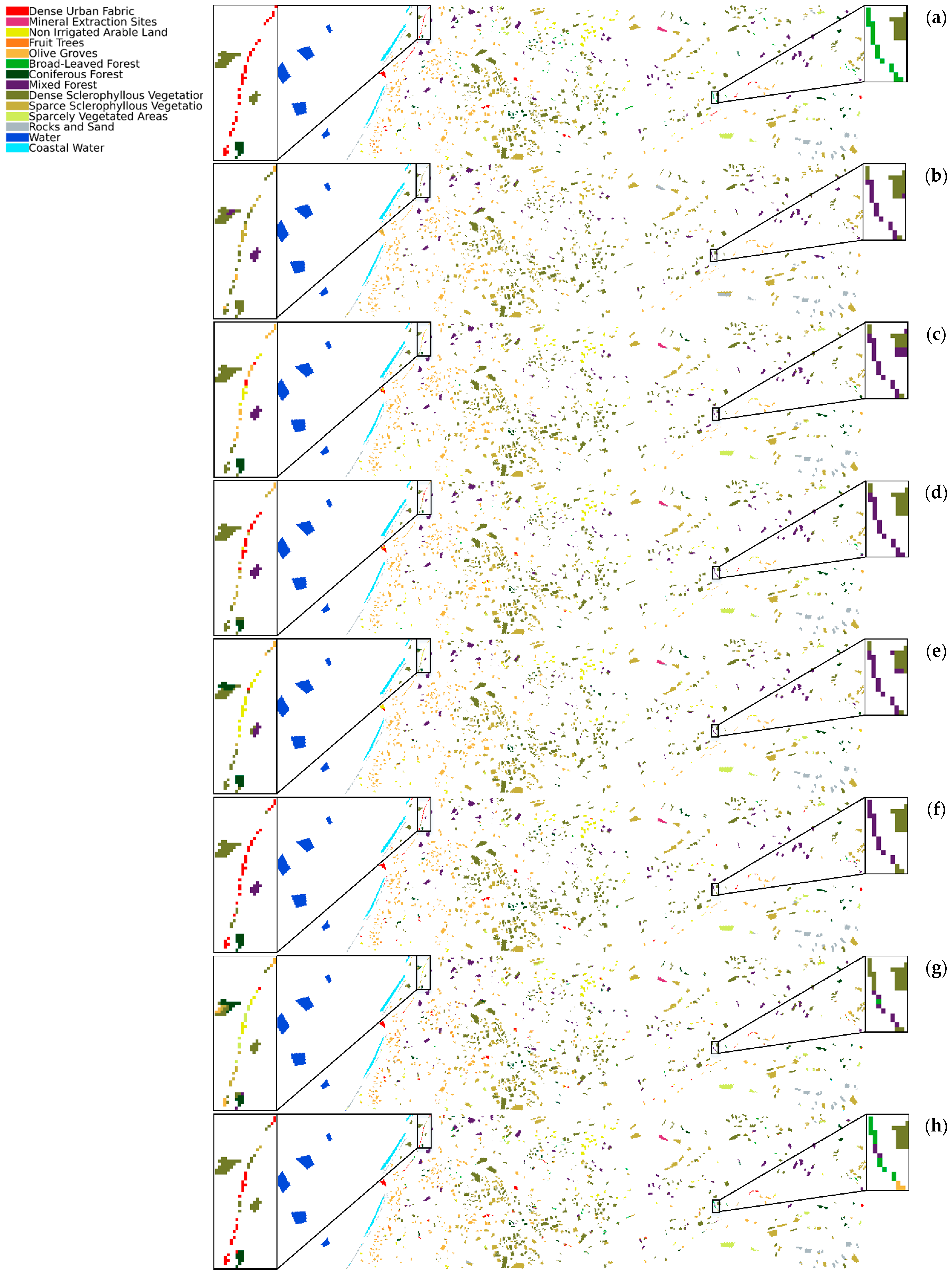
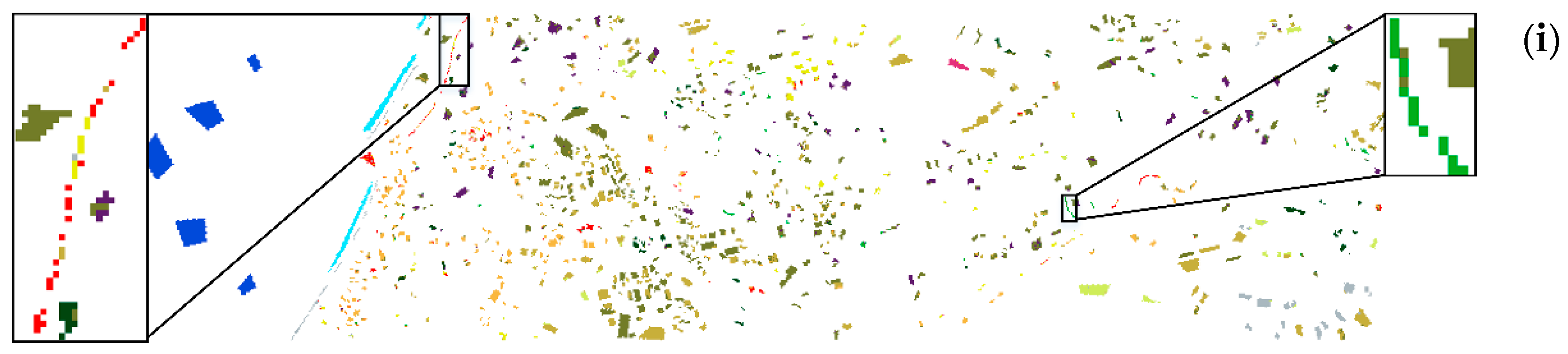
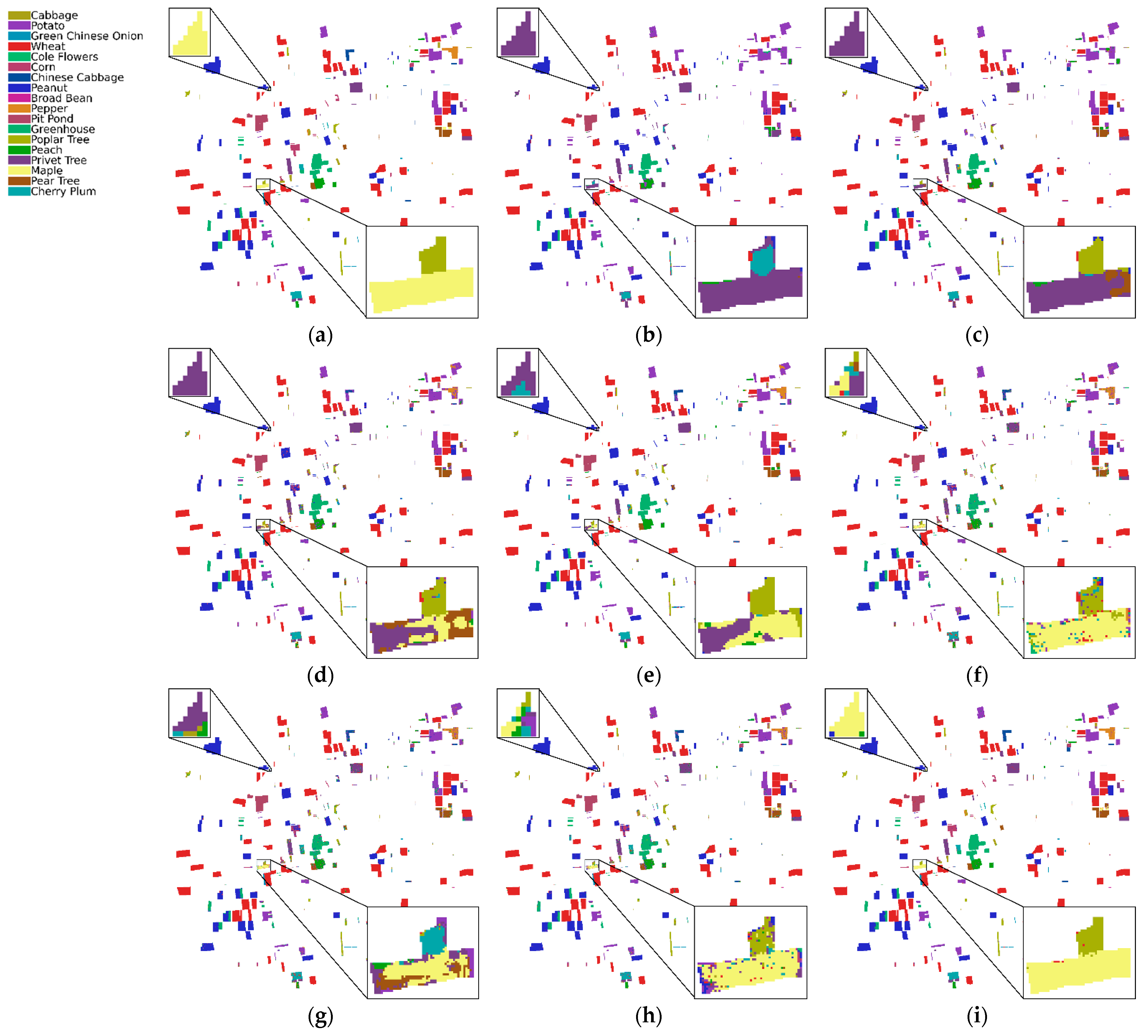
In addition to OA, AA, Kappa, and other indicators, we can also intuitively view the classification performance of the classification model from the classification result graph. The classification results of several algorithms on the two datasets are shown in Figure 6 and Figure 7.

Figure 6 shows that SSACT has relatively few noise points. In order to better illustrate the classification effect, we have enlarged some areas. From the left enlarged region, it can be seen that supervised classification algorithms such as SSRN have poor classification results for class 1 and SSACT and SSAN have better classification results for class 1. From the enlarged area on the right side, it can be seen that SSACT can better classify class 6 and obtain a pleasing ‘Green’, while other algorithms have poor classification results. This is because the number of training samples for class 6 is small, which also shows the role of Class-IoU in solving the problem of class imbalance.

The GF14 satellite hyperspectral image dataset is the closest to the practical application. The distribution of different objects is obtained by field mapping. The cost of obtaining labeled samples is very high, but it gives us an important reference for satellite hyperspectral image classification research. From the overall classification effect, the noise and misclassification of SSACT are less than other algorithms, reflecting better classification performance. We have enlarged some of the classification results for class 16. From the left enlarged region, it can be seen that the classification effect of the seven comparison algorithms on class 16 is not ideal. It is common to misclassify class 16 into category 15, indicating that there are similar features between class 16 and class 15, and the classifier is difficult to distinguish. Note that SSACT can better distinguish between class 16 and class 15, which fully shows that the spatial–spectral–associative contrastive learning framework proposed in this paper can better extract diagnostic features, thereby enhancing the classification performance of the classifier.

4. Discussion

4.1. Classification with Sufficient Samples

This paper focuses on achieving high-accuracy classification under small sample conditions, but it does not mean that our algorithm will deviate from the processing of sufficient samples. We randomly selected 90% of the samples from the two datasets of HL and GF14 for training, and the classification results are shown in

Table 5. Classification results (%) by selecting 90% labeled samples.

Criteria	HL	GF14
OA	99.17	99.74
AA	99.19	99.50
Kappa	99.02	99.67

. The classification performance on the two datasets exceeds 99%; especially, the overall classification accuracy of the GF14 satellite hyperspectral image reaches 99.67%, which fully suggests that the model has a powerful ability to learn data features in the associative contrastive learning stage, and provides a feature representation with strong separability for the classifier. Excellent classification performance can be achieved under both sufficient and small samples. Furthermore, the models can accurately classify two datasets with disparate spatial scales, indicating that the model can classify not only small-scale hyperspectral images such as by traditional classification algorithms but also large-scale satellite hyperspectral images.

4.2. Classification without Class-IoU

It can be seen from the previous experimental results that the Class-IoU has significantly improved the classification performance of the class with a small number of samples. To further illustrate the effectiveness of in solving the class instability problem, we only use the Cross-Entropy loss function to train the classifier, excluding the use of Class-IoU. The classification results are shown in

Table 6. Average Accuracy results (%) by selecting 10% labeled samples.

Criteria	HL	GF14
Only Cross-Entropy	81.28	81.51
With Class-IoU	83.63	85.15

. From the experimental results of the two datasets, it can be seen that the performance of classifiers using only the Cross-Entropy loss function on AA becomes less satisfying than that of classifiers using the Class-IoU loss function. It should be noted that when only using the Cross-Entropy loss function, the classification performance is also superior to other algorithms, which also shows that the spatial–spectral associate contrastive learning module proposed in this paper can obtain diagnostic separability features for different classes.

4.3. Classification with Spatial/Spectral Contrastive Learning Module

To illustrate the important role of the associative spatial–spectral contrastive learning module, we compared the classification performance of only using the spatial or spectral contrastive learning module. The experimental results are shown in

Table 7. Classification results (%) by 10% labeled samples with different modules.

Criteria	HL			GF14
	Spatial	Spectral	Spatial-Spectral	Spatial	Spectral	Spatial-Spectral
OA	69.40	66.19	84.74	84.29	75.34	93.21
AA	68.71	64.95	83.63	73.37	40.84	85.15
Kappa	63.68	58.69	81.78	79.51	67.88	91.27

. From the experimental results, it can be seen that the classification effect on HL and GF14 datasets are not ideal when only using the spatial or spectral contrastive learning module; especially, the AA of classification is far lower than using the associative spatial–spectral contrastive learning module. From the datasets, the spatial resolution of the HL dataset is lower than GF14, resulting in the widespread existence of mixed pixels. Therefore, when only using spatial or spectral information, the classification accuracy is poor on HL datasets. Similar to the Adaboost strategy, the associative spatial–spectral contrastive learning module can provide more separability features for downstream classification tasks based on spatial and spectral features. The experimental results also show that the classification accuracy is significantly improved.

4.4. Disadvantages

First of all, we effectively improved the classification accuracy of the classes with a small number of samples by adding the Class-IoU constraint to the classification loss function, but the classification accuracy of the classes with a large number of samples is decreased. This is also a difficult problem to balance in practical applications. In the future, we will continue to study and improve this scheme. Secondly, in contrastive learning, we consider the mutual constraints of spatial and spectral features, but the relationship between cross-domain features is not fully explored. The spatial–spectral cross-contrastive learning process can be increased to extract cross-domain invariant features, which will be tested in subsequent studies. Finally, our algorithm has no advantage in running time. Taking GF14 datasets as an example, the implementation takes around 118 min, which includes self-supervised feature extraction and classification training.

5. Conclusions

In this paper, we propose a satellite hyperspectral image classification method based on spatial–spectral associative contrastive learning, which can effectively extract the spatial and spectral features from hyperspectral data. SSACT can solve the problem of class imbalance, which significantly improves the classification accuracy of classes with a small number of samples. Based on the Transformer architecture, we construct spatial and spectral contrastive learning networks and downstream classifiers. The experimental results also prove that the excellent feature extraction ability of the Transformer is helpful to improve the classification performance. In terms of AA, the performance of SSACT on the two datasets is 83.63% and 85.15%, respectively, which is 26.74% and 43.1% higher than other algorithms on average.

References

1. Transon, J.; D’Andrimont, R.; Maugnard, A.; Defourny, P. Survey of Hyperspectral Earth Observation Applications from Space in the Sentinel-2 Context. Remote. Sens. 2018, 10, 157. [Google Scholar] [CrossRef] [Green Version]
2. Pearlman, J.S.; Barry, P.S.; Segal, C.C.; Shepanski, J.; Beiso, D.; Carman, S.L. Hyperion, a space-based imaging spectrometer. IEEE Trans. Geosci. Remote Sens. 2003, 41, 1160–1173. [Google Scholar] [CrossRef]
3. Wang, Q.; Wu, C.; Li, Q.; Li, J. Chinese HJ-1A/B satellites and data characteristics. Sci. China Earth Sci. 2010, 53, 51–57. [Google Scholar] [CrossRef]
4. Qin, Y.; Zhang, X.; Zhao, Z.; Li, Z.; Yang, C.; Huang, Q. Coupling Relationship Analysis of Gold Content Using Gaofen-5 (GF-5) Satellite Hyperspectral Remote Sensing Data: A Potential Method in Chahuazhai Gold Mining Area, Qiubei County, SW China. Remote Sens. 2022, 14, 109. [Google Scholar] [CrossRef]
5. Guo, Y.; Mokany, K.; Ong, C.; Moghadam, P.; Ferrier, S.; Levick, S. Quantitative Assessment of DESIS Hyperspectral Data for Plant Biodiversity Estimation in Australia. In Proceedings of the IGARSS 2022—2022 IEEE International Geoscience and Remote Sensing Symposium, Kuala Lumpur, Malaysia, 17–22 July 2022; pp. 1744–1747. [Google Scholar]
6. Loizzo, R.; Guarini, R.; Longo, F.; Scopa, T.; Formaro, R.; Facchinetti, C.; Varacalli, G. Prisma: The Italian Hyperspectral Mission. In Proceedings of the IGARSS 2018—2018 IEEE International Geoscience and Remote Sensing Symposium, Valencia, Spain, 22–27 July 2018; pp. 175–178. [Google Scholar]
7. Qin, J.; Zhao, H.; Liu, B. Self-Supervised Denoising for Real Satellite Hyperspectral Imagery. Remote Sens. 2022, 14, 3083. [Google Scholar] [CrossRef]
8. Sethy, P.K.; Pandey, C.; Sahu, Y.K.; Behera, S.K. Hyperspectral imagery applications for precision agriculture—A systemic survey. Multimed. Tools Appl. 2022, 81, 3005–3038. [Google Scholar] [CrossRef]
9. You, M.; RuoFei, Z.; Shisong, C. Orbita hyperspectral satellite image for land cover classification using random forest classifier. J. Appl. Remote Sens. 2021, 15, 014519. [Google Scholar]
10. Zhang, L.; Zhang, L.; Du, B.; You, J.; Tao, D. Hyperspectral image unsupervised classification by robust manifold matrix factorization. Inf. Sci. 2019, 485, 154–169. [Google Scholar] [CrossRef]
11. Kruse, F.A.; Lefkoff, A.; Boardman, J.; Heidebrecht, K.; Shapiro, A.; Barloon, P.; Goetz, A. The spectral image processing system (SIPS)—Interactive visualization and analysis of imaging spectrometer data. Remote Sens. Environ. 1993, 44, 145–163. [Google Scholar] [CrossRef]
12. Richards, J.; Jia, X. Remote Sensing Digital Image Analysis; Springer: Berlin/Heidelberg, Germany, 2006. [Google Scholar]
13. Bruzzone, L.; Demir, B. A review of modern approaches to classification of remote sensing data. Land Use Land Cover. Mapp. Eur. Pract. Trends 2014, 18, 127–143. [Google Scholar]
14. Falco, N.; Benediktsson, J.A.; Bruzzone, L. Spectral and Spatial Classification of Hyperspectral Images Based on ICA and Reduced Morphological Attribute Profiles. IEEE Trans. Geosci. Remote Sens. 2015, 53, 6223–6240. [Google Scholar] [CrossRef] [Green Version]
15. Xia, J.; Mura, M.D.; Chanussot, J.; Du, P.; He, X. Random Subspace Ensembles for Hyperspectral Image Classification With Extended Morphological Attribute Profiles. IEEE Trans. Geosci. Remote Sens. 2015, 53, 4768–4786. [Google Scholar] [CrossRef]
16. Cao, X.; Xu, Z.; Meng, D. Spectral-Spatial Hyperspectral Image Classification via Robust Low-Rank Feature Extraction and Markov Random Field. Remote Sens. 2019, 11, 1565. [Google Scholar] [CrossRef] [Green Version]
17. Zhong, Z.; Li, J.; Luo, Z.; Chapman, M. Spectral–spatial residual network for hyperspectral image classification: A 3-D deep learning framework. IEEE Trans. Geosci. Remote Sens. 2017, 56, 847–858. [Google Scholar] [CrossRef]
18. Chen, Y.; Lin, Z.; Zhao, X.; Wang, G.; Gu, Y. Deep Learning-Based Classification of Hyperspectral Data. IEEE J. Sel. Top. Appl. Earth Obs. Remote Sens. 2014, 7, 2094–2107. [Google Scholar] [CrossRef]
19. Chen, Y.; Zhao, X.; Jia, X. Spectral–Spatial Classification of Hyperspectral Data Based on Deep Belief Network. IEEE J. Sel. Top. Appl. Earth Obs. Remote Sens. 2015, 8, 2381–2392. [Google Scholar] [CrossRef]
20. Li, S.; Song, W.; Fang, L.; Chen, Y.; Ghamisi, P.; Benediktsson, J.A. Deep Learning for Hyperspectral Image Classification: An Overview. IEEE Trans. Geosci. Remote Sens. 2019, 57, 6690–6709. [Google Scholar] [CrossRef] [Green Version]
21. Cheng, G.; Li, Z.; Han, J.; Yao, X.; Guo, L. Exploring Hierarchical Convolutional Features for Hyperspectral Image Classification. IEEE Trans. Geosci. Remote Sens. 2018, 56, 6712–6722. [Google Scholar] [CrossRef]
22. Chen, Y.; Jiang, H.; Li, C.; Jia, X.; Ghamisi, P. Deep Feature Extraction and Classification of Hyperspectral Images Based on Convolutional Neural Networks. IEEE Trans. Geosci. Remote Sens. 2016, 54, 6232–6251. [Google Scholar] [CrossRef] [Green Version]
23. Hamida, A.B.; Benoit, A.; Lambert, P.; Amar, C.B. 3-D Deep Learning Approach for Remote Sensing Image Classification. IEEE Trans. Geosci. Remote Sens. 2018, 56, 4420–4434. [Google Scholar] [CrossRef] [Green Version]
24. Tang, G.; Müller, M.; Rios Gonzales, A.; Sennrich, R. Why Self-Attention? A Targeted Evaluation of Neural Machine Translation Architectures. In Proceedings of the 2018 Conference on Empirical Methods in Natural Language Processing, Brussels, Belgium, 31 October—4 November 2018; pp. 4263–4272. [Google Scholar]
25. Vaswani, A.; Shazeer, N.M.; Parmar, N.; Uszkoreit, J.; Jones, L.; Gomez, A.N.; Kaiser, L.; Polosukhin, I. Attention is All you Need. arXiv 2017, arXiv:1706.03762. [Google Scholar]
26. Dosovitskiy, A.; Beyer, L.; Kolesnikov, A.; Weissenborn, D.; Zhai, X.; Unterthiner, T.; Dehghani, M.; Minderer, M.; Heigold, G.; Gelly, S.; et al. An Image is Worth 16 × 16 Words: Transformers for Image Recognition at Scale. arXiv 2021, arXiv:2010.11929. [Google Scholar]
27. He, X.; Chen, Y.; Lin, Z. Spatial-Spectral Transformer for Hyperspectral Image Classification. Remote Sens. 2021, 13, 498. [Google Scholar] [CrossRef]
28. Qing, Y.; Liu, W.; Feng, L.; Gao, W. Improved Transformer Net for Hyperspectral Image Classification. Remote Sens. 2021, 13, 2216. [Google Scholar] [CrossRef]
29. Yang, X.; Cao, W.; Lu, Y.; Zhou, Y. Hyperspectral Image Transformer Classification Networks. IEEE Trans. Geosci. Remote Sens. 2022, 60, 5528715. [Google Scholar] [CrossRef]
30. Zou, J.; He, W.; Zhang, H. LESSFormer: Local-Enhanced Spectral-Spatial Transformer for Hyperspectral Image Classification. IEEE Trans. Geosci. Remote Sens. 2022, 60, 5535416. [Google Scholar] [CrossRef]
31. Tu, B.; Liao, X.; Li, Q.; Peng, Y.; Plaza, A.J. Local Semantic Feature Aggregation-Based Transformer for Hyperspectral Image Classification. IEEE Trans. Geosci. Remote Sens. 2022, 60, 5536115. [Google Scholar] [CrossRef]
32. Wang, G.; Ren, P. Hyperspectral Image Classification with Feature-Oriented Adversarial Active Learning. Remote Sens. 2020, 12, 3879. [Google Scholar] [CrossRef]
33. Oord, A.v.d.; Li, Y.; Vinyals, O. Representation Learning with Contrastive Predictive Coding. arXiv 2018, arXiv:1807.03748. [Google Scholar]
34. Chen, T.; Kornblith, S.; Norouzi, M.; Hinton, G.E. A Simple Framework for Contrastive Learning of Visual Representations. arXiv 2020, arXiv:2002.05709. [Google Scholar]
35. Wang, Y.; Mei, J.; Zhang, L.; Zhang, B.; Zhu, P.; Li, Y.; Li, X. Self-Supervised Feature Learning With CRF Embedding for Hyperspectral Image Classification. IEEE Trans. Geosci. Remote Sens. 2019, 57, 2628–2642. [Google Scholar] [CrossRef]
36. Zhu, M.; Fan, J.; Yang, Q.; Chen, T. SC-EADNet: A Self-Supervised Contrastive Efficient Asymmetric Dilated Network for Hyperspectral Image Classification. IEEE Trans. Geosci. Remote Sens. 2022, 60, 1–17. [Google Scholar] [CrossRef]
37. Liu, B.; Yu, A.; Yu, X.; Wang, R.; Gao, K.; Guo, W. Deep Multiview Learning for Hyperspectral Image Classification. IEEE Trans. Geosci. Remote Sens. 2021, 59, 7758–7772. [Google Scholar] [CrossRef]
38. Hou, S.; Shi, H.; Cao, X.; Zhang, X.; Jiao, L. Hyperspectral Imagery Classification Based on Contrastive Learning. IEEE Trans. Geosci. Remote Sens. 2022, 60, 5521213. [Google Scholar] [CrossRef]
39. Guan, P.; Lam, E.Y. Cross-Domain Contrastive Learning for Hyperspectral Image Classification. IEEE Trans. Geosci. Remote Sens. 2022, 60, 5528913. [Google Scholar] [CrossRef]
40. Hu, X.; Li, T.; Zhou, T.; Liu, Y.; Peng, Y. Contrastive Learning Based on Transformer for Hyperspectral Image Classification. Appl. Sci. 2021, 11, 8670. [Google Scholar] [CrossRef]
41. Zhang, T.; Qiu, C.; Ke, W.; Süsstrunk, S.; Salzmann, M. Leverage Your Local and Global Representations: A New Self-Supervised Learning Strategy. In Proceedings of the 2022 IEEE/CVF Conference on Computer Vision and Pattern Recognition (CVPR), New Orleans, Louisiana, 18–24 June 2022; pp. 16559–16568. [Google Scholar]
42. Karantzalos, K.; Karakizi, C.; Kandylakis, Z.; Antoniou, G. Hyrank Hyperspectral Satellite Dataset I. 2018. Available online: https://zenodo.org/record/1222202#.ZBKEwnYzaUk (accessed on 13 March 2023).
43. Bazi, Y.; Bashmal, L.; Rahhal, M.M.A.; Dayil, R.A.; Ajlan, N.A. Vision Transformers for Remote Sensing Image Classification. Remote Sens. 2021, 13, 516. [Google Scholar] [CrossRef]
44. Xu, X.; Feng, Z.; Cao, C.; Li, M.; Wu, J.; Wu, Z.; Shang, Y.; Ye, S. An Improved Swin Transformer-Based Model for Remote Sensing Object Detection and Instance Segmentation. Remote Sens. 2021, 13, 4779. [Google Scholar] [CrossRef]
45. Xu, Z.; Zhang, W.; Zhang, T.; Yang, Z.; Li, J. Efficient Transformer for Remote Sensing Image Segmentation. Remote Sens. 2021, 13, 3585. [Google Scholar] [CrossRef]
46. Zhang, C.; Wang, L.; Cheng, S.; Li, Y. SwinSUNet: Pure Transformer Network for Remote Sensing Image Change Detection. IEEE Trans. Geosci. Remote Sens. 2022, 60, 5224713. [Google Scholar] [CrossRef]
47. Hong, D.; Han, Z.; Yao, J.; Gao, L.; Zhang, B.; Plaza, A.; Chanussot, J. SpectralFormer: Rethinking Hyperspectral Image Classification With Transformers. IEEE Trans. Geosci. Remote Sens. 2022, 60, 1–15. [Google Scholar] [CrossRef]
48. Sawant, S.S.; Manoharan, P. Unsupervised band selection based on weighted information entropy and 3D discrete cosine transform for hyperspectral image classification. Int. J. Remote Sens. 2020, 41, 3948–3969. [Google Scholar] [CrossRef]
49. Wu, Y.; Zhou, Y.; Saveriades, G.; Agaian, S.; Noonan, J.P.; Natarajan, P. Local Shannon entropy measure with statistical tests for image randomness. Inf. Sci. 2013, 222, 323–342. [Google Scholar] [CrossRef] [Green Version]
50. Tolstikhin, I.O.; Houlsby, N.; Kolesnikov, A.; Beyer, L.; Zhai, X.; Unterthiner, T.; Yung, J.; Keysers, D.; Uszkoreit, J.; Lucic, M.; et al. MLP-Mixer: An all-MLP Architecture for Vision. Adv. Neural Inf. Process. Syst. 2021, 34, 24261–24272. [Google Scholar]
51. Touvron, H.; Bojanowski, P.; Caron, M.; Cord, M.; El-Nouby, A.; Grave, E.; Izacard, G.; Joulin, A.; Synnaeve, G.; Verbeek, J.; et al. ResMLP: Feedforward Networks for Image Classification With Data-Efficient Training. IEEE Trans. Pattern Anal. Mach. Intell. 2022, 45, 5314–5321. [Google Scholar] [CrossRef] [PubMed]
52. Roy, S.K.; Krishna, G.; Dubey, S.R.; Chaudhuri, B.B. HybridSN: Exploring 3-D–2-D CNN Feature Hierarchy for Hyperspectral Image Classification. IEEE Geosci. Remote Sens. Lett. 2020, 17, 277–281. [Google Scholar] [CrossRef] [Green Version]
53. Sun, H.; Zheng, X.; Lu, X.; Wu, S. Spectral–Spatial Attention Network for Hyperspectral Image Classification. IEEE Trans. Geosci. Remote Sens. 2020, 58, 3232–3245. [Google Scholar] [CrossRef]
54. Chen, H.; Li, X.; Zhou, J.; Wang, Y. TPPI: A Novel Network Framework and Model for Efficient Hyperspectral Image Classification. Photogramm. Eng. Remote Sens. 2022, 88, 535–546. [Google Scholar] [CrossRef]
Figure 1. HL dataset false color images and ground truth. (a) three-band composite false color images (23, 11, 7); (b) ground truth.
Remotesensing 15 01612 g001
Figure 2. GF14 dataset false color images and ground truth: (a) three-band composite false color images (25, 11, 7); (b) ground truth.
Remotesensing 15 01612 g002
Figure 3. Workflow of the proposed method. (a) Generate data cube patches. (b) Image entropy and data augmentation. (c) Spatial and spectral patch embeddings. (d) Spatial-spectral associative contrastive learning and Class-IoU. (e) HSI Classification.
Remotesensing 15 01612 g003
Figure 4. Comparison of band information with maximum image entropy and minimum image entropy. (a) band = 1, image entropy = 5.37; (b) band = 50, image entropy = 9.24.
Remotesensing 15 01612 g004
Figure 5. Class-IoU. TP: The number of Wheat correctly classified. FP: The number of classifier misclassifications. TN: The number of non-Wheat correctly classified. FN: The number of classifiers missed.
Remotesensing 15 01612 g005
Figure 6. Classification results of different algorithms on the HL dataset: (a) ground truth; (b) 2D-CNN; (c) 3D-CNN; (d) SSRN; (e) HybridSN; (f) SSAN; (g) ViT; (h) DMVL; (i) SSACT.
Remotesensing 15 01612 g006aRemotesensing 15 01612 g006b
Figure 7. Classification results of different algorithms on the GF14 dataset: (a) ground truth; (b) 2D-CNN; (c) 3D-CNN; (d) SSRN; (e) HybridSN; (f) SSAN; (g) ViT; (h) DMVL; (i) SSACT.
Remotesensing 15 01612 g007