Article

Unlocking the Potential of Data Augmentation in Contrastive Learning for Hyperspectral Image Classification

College of Electrical Engineering, Zhejiang University, Hangzhou 310027, China
*
Author to whom correspondence should be addressed.
Remote Sens. 2023, 15(12), 3123; https://doi.org/10.3390/rs15123123
Submission received: 14 May 2023 / Revised: 7 June 2023 / Accepted: 8 June 2023 / Published: 15 June 2023
(This article belongs to the Special Issue Advances in Hyperspectral Data Exploitation II)

Abstract

:
Despite the rapid development of deep learning in hyperspectral image classification (HSIC), most models require a large amount of labeled data, which are both time-consuming and laborious to obtain. However, contrastive learning can extract spatial–spectral features from samples without labels, which helps to solve the above problem. Our focus is on optimizing the contrastive learning process and improving feature extraction from all samples. In this study, we propose the Unlocking-the-Potential-of-Data-Augmentation (UPDA) strategy, which involves adding superior data augmentation methods to enhance the representation of features extracted by contrastive learning. Specifically, we introduce three augmentation methods—band erasure, gradient mask, and random occlusion—to the Bootstrap-Your-Own-Latent (BYOL) structure. Our experimental results demonstrate that our method can effectively improve feature representation and thus improve classification accuracy. Additionally, we conduct ablation experiments to explore the effectiveness of different data augmentation methods.

1. Introduction

Hyperspectral images (HSI) have gained widespread use due to their ability to provide extensive spectral and spatial information [1]. With hundreds of bands, HSIs can distinguish surface materials based on their unique spectral characteristics with exceptional spectral resolution. This feature makes them highly valuable for various applications, including vegetation surveys, atmospheric research, military detection, environmental monitoring [2] and landcover classification [3]. HSIC is a key research area within the hyperspectral field and involves the classification of individual pixels based on the rich spectral information they contain. As hardware technology continues to improve, the spatial resolution of hyperspectral sensors also increases, allowing for the incorporation of spatial information from surrounding pixels in classification efforts. Currently, the combination of spectral and spatial features is the primary approach in the HSIC field [4].
The abundance of bands in HSI presents a significant challenge in classification. Processing such large amounts of data directly without reduction would require a network of immense scale and huge computational memory. Furthermore, high spectral resolution creates spectral redundancy, which can be addressed through dimensionality reduction techniques that preserve critical information while reducing data size. Feature extraction is a widely used method for reducing data dimensions in HSI by extracting or sorting effective features for subsequent use. Common methods for feature extraction include principal component analysis (PCA) [5], independent component analysis (ICA) [6], linear discriminant analysis (LDA) [7], multidimensional scaling (MDS) [8], etc. These algorithms are still widely used as preprocessing methods due to their simplicity and effectiveness. With the increasing maturity of deep learning algorithms, more sophisticated algorithms are being developed to extract features from HSIs. Presently, the prevalent classification method involves using supervised or unsupervised feature extraction algorithms to extract spectral or spatial–spectral features, followed by classifier training using the extracted features.
The earlier developed feature extraction algorithms were based on supervised deep learning. In supervised learning, convolutional neural networks (CNNs) play an crucial role, evolving from one-dimensional CNNs [9] that only extract spectral features to two-dimensional and three-dimensional CNNs [10] that extract both spatial and spectral information. Roy et al. proposed the HybridSN network, which combines 2D and 3D convolutions to further enhance classification accuracy [11]. Zhong et al. introduced the classic residual network into the hyperspectral domain and designed the SSRN network [12]. Zhong et al. combined attention mechanism and CNNs [13]. Apart from CNNs, deep recurrent neural networks (DRNN) [14], deep feed-forward networks (DFFN), and other networks have also achieved promising results in HSIC.
However, supervised learning often heavily relies on labeled data, necessitating a sufficient number of labeled samples to achieve optimal training results. In the case of HSIs, both data collection and labeling involve significant human and time costs. Consequently, in recent years, the focus of feature extraction algorithms has gradually shifted towards unsupervised deep learning. The fundamental difference between unsupervised learning and supervised learning lies in the fact that the training data of unsupervised learning are unlabeled, and samples are classified based on their similarities, reducing the distance between data of the same class and increasing the distance between data of different classes. Without the constraints of labels, unsupervised learning can unleash the potential of models, enabling them to autonomously discover and explore data, learn more latent features, and ultimately result in models with better robustness and generalization. Unsupervised learning can be divided into generative learning and discriminative learning. Generative models learn to model the underlying probability distribution of input data. They are trained on large amounts of data and leverage this information to synthesize new samples that resemble the original data. The most basic generative deep learning algorithms include autoencoders (AE) [15] and generative adversarial networks (GAN) [16]. Variants of AEs, such as the adversarial autoencoder (AAE) [17], variational autoencoder (VAE) [18], and masked autoencoder (MAE) [19], have been widely used for feature extraction in hyperspectral image analysis. GANs optimized with algorithms such as deep convolutional GAN (DCGAN) [20], information maximizing GAN (InfoGAN) [21], and multitask GAN [22] have also achieved remarkable results in HSIC.
Discriminative learning models the conditional probability and learns the optimal boundary between different classes. Contrastive learning is a typical discriminative learning algorithm in deep learning, which aims to acquire representations by contrasting positive and negative pairs in the latent space. Positive pairs are spatially close but spectrally similar patches, whereas negative pairs are either spectrally dissimilar or spatially distant patches. By minimizing the distance between positive pairs and maximizing the distance between negative pairs, the model learns to encode both spatial and spectral information in the latent space.
Contrastive learning has made rapid progress in recent years, and many variants such as Moco [23], SimCLR [24], BYOL [25], SwAV [26], and SimSiam [27] have been proposed and gradually applied in the field of hyperspectral data analysis [28]. These methods differ in their choice of contrastive loss, encoder architecture, and training strategy. However, they share a common goal of learning representations that capture the underlying structure of hyperspectral data. Furthermore, the key to contrastive learning is to prevent model collapse, which means that all data converge to the same constant solution after feature representation.
For contrastive learning, we can integrate additional optimization techniques to encourage the model to learn more representative features while ensuring that it does not collapse. In handling the spatial–spectral features of HSIs, spatial and spectral information are often combined into the same sample. Although this approach is simple and compensates for the lack of spectral information, directly inputting the entire sample cube into the model results in a significant amount of redundant information interfering with feature extraction. Some studies have separated spatial and spectral information into different samples and used cross-domain contrastive learning to extract them separately [28,29,30]. This approach can reduce a lot of redundant information but may also lead to the loss of valuable sub-key information. Coordinating the extraction of spatial and spectral information, preserving useful information as much as possible, reducing the interference of useless information, and increasing the model’s attention to key information are essential for improving the efficiency of contrastive learning.
In this study, we incorporated multiple optimization strategies into contrastive learning to improve feature extraction. These strategies include band erasure (BE), random occlusion (RO) [31], and gradient mask (GM). The motivation of our study is to greatly improve the feature extraction effect and unlock the potential of the model by adding new data augmentation methods while the model remains unchanged. Experimental results have shown that each of these strategies can significantly improve feature performance and classification accuracy. Furthermore, when combined, they can lead to unexpected improvements.
In the following sections, we will first introduce the relevant algorithms’ background knowledge (Section 2). Then, we will provide a detailed description of our proposed method’s overall framework and each module (Section 3). Next, we will describe and analyze our comparative and ablation experiments (Section 4). Finally, we will present our conclusions (Section 5). The main contributions of this study are as follows:
(1)
We propose the band erasure strategy to improve spectral features extracted by contrastive learning.
(2)
We propose the gradient masking strategy to enhance the model’s attention to key areas, reduce attention to edge positions, and minimize the interference of useless information on features.
(3)
We propose the Unlocking-the-Potential-of-Data-Augmentation (UPDA) strategy, which involves adding superior data augmentation methods to improve the features extracted by contrastive learning. We used UPDA in the BYOL structure and improved the classification accuracy to a new level.

2. Related Work

2.1. Contrastive Learning

Contrastive learning is a type of self-supervised learning that involves constructing pairs of similar and dissimilar examples to learn a representation learning model. The goal is to learn a model that projects similar samples close together in a projection space, whereas dissimilar samples are projected far apart. Essential factors in contrastive learning include how to construct similar and dissimilar samples, how to design a representation learning model that adheres to the above principles, and how to prevent model collapse, which occurs when all data converge to a single constant solution after feature representation. Currently, there are many contrastive learning methods available, and they can be roughly categorized into those based on negative samples [24], contrastive clustering [26], asymmetric network structures [25,27], and redundancy elimination loss functions, depending on the approach used to prevent model collapse.
Bootstrap-Your-Own-Latent (BYOL) is a typical asymmetric structure-based approach, where the online network has an extra predictor compared to the target network. Furthermore, the two branches are connected by an asymmetric similarity loss. BYOL extracts features of samples by training the ability of online network to predict the output of target network, thereby learning the potential connections between positive sample pairs. Unlike other contrastive learning methods, BYOL only requires positive sample pairs, not negative ones, which makes the BYOL model more robust and generalizable.
He et al. proposed Simsiam [27] and analyzed the necessary factors to make the network not collapse. Its structure is similar to BYOL, retaining the predictor of the online network, but without EMA (exponential moving average). Simsiam proves that EMA is not necessary to prevent collapse but removing it will sacrifice part of the accuracy [32].
In this work, in order to achieve better classification accuracy, we continue to use the BYOL structure.

2.2. Data Augmentation

2.2.1. Normal Data Augmentation

Data augmentation is a widely used technique in contrastive learning that increases the diversity of the training data by creating new samples that are variations of the original data. This technique helps to reduce overfitting and improve the model’s ability to generalize. In contrastive learning, data augmentation is typically applied to both the anchor and positive samples to create new pairs of samples for training.
Normal augmentation methods, such as random cropping, flipping, rotation, color jittering, and Gaussian noise injection, are often used in contrastive learning [33]. The augmented samples are paired with their corresponding original samples to form positive pairs for training, thereby increasing the number of positive pairs and enhancing the diversity of the training data. This can improve the performance of the contrastive learning model.
Although they can be used to process hyperspectral data, these normal augmentation methods were originally designed for RGB or grayscale images and do not take into account the unique characteristics of HSIs.
In [34], the author pointed out that in the existing contrastive learning, it is not ideal to use various data augmentation methods to map the original data to the same space and then perform various downstream tasks. Blindly using data augmentation methods may be harmful to the learned features. We believe that the choice of data augmentation method should be based on the specific downstream tasks and the shape of the data. To fully leverage the potential of contrastive learning in HSIC, it is necessary to develop new data augmentation techniques that are tailored to hyperspectral data.

2.2.2. Random Occlusion

The random occlusion (RO) technique is a data augmentation method that involves randomly masking or occluding a portion of the input data during training. This technique simulates missing or incomplete information in the input data and forces the model to learn robust features that can still accurately classify the data, even when certain regions are missing. Random occlusion can be applied to various types of input data, such as images, text, and audio. In image classification tasks, random occlusion can be applied by randomly masking a portion of the image with a black rectangle or by replacing a portion of the image with random noise. The size and location of the occluded region can also be randomized to increase the diversity of the training data. By using random occlusion as a data augmentation technique, the model can learn to be more robust to incomplete or missing data, which can improve its performance on real-world situations where the input data may be noisy or incomplete.
When we were thinking about how to extract more representative features, we tried to explain why traditional augmentation methods make sense in feature extraction. We suspected that when using color distortion, we can encourage models to pay more attention to features except color, and when using Gaussian noise, we can tell our models to not be obsessed with small, discrete morphological features. We guessed that if we occlude an uncritical area, the model will pay more attention to the rest. So, as long as we do not occlude the features at key positions, the model can extract better space features.
RO was first used in HSIC in [31], where Haut et al. applied this technique to a CNN network and demonstrated its effectiveness. In our previous work [35], we integrated random occlusion into the BYOL structure for HSIC and achieved significant improvements in classification accuracy across various datasets.
Based on previous experiments, we have proved that proper occlusion strategies can improve results effectively when applied to HSIC. For our experiments, when the occlusion value is set to 1, and the area set to 10% of the patch area, the network works best.

3. Method

In this section, we provide a detailed introduction to the UPDA method and its application in the BYOL structure. Specifically, we first present the overall framework of the proposed method, followed by a detailed explanation of the newly proposed data augmentation methods, band erasure and gradient mask. Finally, we describe in detail the process of contrastive learning training and training of a classifier using the extracted features.

3.1. Framework of the Method

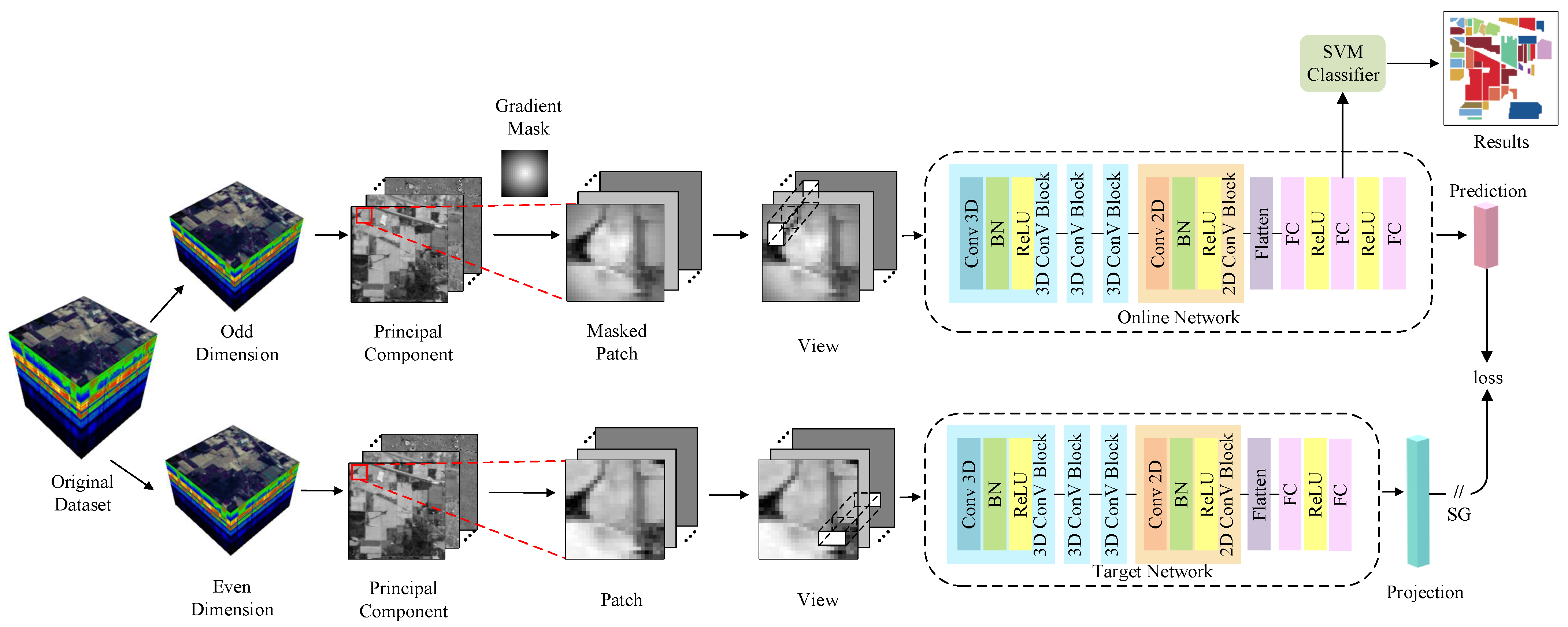
Figure 1 illustrates the framework of the proposed method, which mainly consists of the UPDA process and the contrastive learning feature extraction process, with the former including data preprocessing.
Let  X R h × w × c  be the original input hyperspectral image, where h and w are the height and width of the image, and c is the number of bands. First, the data are subjected to band erasure, where odd and even layers are erased separately to obtain two parts,  X 0  and  X 1 , forming two branches.
PCA is then performed on each branch to reduce dimensionality, and the resulting samples are segmented into patches:  P 0  and  P 1 . The patches in the upper branch are weighted using a gradient mask, whereas the patches in the lower branch are not processed. Then, both of them are randomly masked to obtain the views  V 0  and  V 1 , which are input into the BYOL structure.
The upper branch of the BYOL structure is an online network, while the lower branch is a target network. The former has an additional linear layer, i.e., the predictor. The loss value is calculated based on the outputs of the upper and lower branches and used to update the network parameters.
After pretraining, the results of the projector are saved as features and input into the SVM classifier for training to complete classification or other downstream tasks. In this way, features are easily migrated between different machines, so that we can extract features on machines with high configuration and complete downstream tasks on any machine. For more detailed information, please refer to the following two subsections.

3.2. Unlocking the Potential of Data Augmentation

3.2.1. Band Erasure

The essence of band erasure is to divide the original HSI into two datasets with non-overlapping bands. In this process, odd and even layers are extracted at intervals, resulting in two datasets that are obtained by erasing half of the bands from the original data and have non-overlapping bands. Band erasure can improve the representativeness of subsequent feature extraction. On the one hand, because hyperspectral data have high spectral resolution and spectral information has a large redundancy, removing half of the bands will not lose critical spectral information and can reduce the interference of redundant information in each branch on feature extraction. On the other hand, the data in the two branches after band erasure are complementary. During the training process of contrastive learning, in order to make the loss function converge, the model tends to focus on shared information and reduce attention to unimportant details. This shared information is often the essential features. We have tried different erasing strategies, such as removing a string of continuous bands or leaving only 1/4 or 1/3 of the total number of bands; however, they are not as effective as the current erasure strategy.
The c spectral bands are divided into  c 0  and  c 1  bands, where  c = c 0 + c 1 , resulting in  X 0 R h × w × c 0  and  X 1 R h × w × c 1 . PCA is then performed on each branch, and the first d principal component maps are selected. The value of d varies depending on the dataset, with 30 for the IP dataset and 15 for the PU and SA datasets. The principal component maps are then segmented into patches using a sliding window of size  s × s  with a stride of 1, resulting in  s × s × d  cubes. Here, s is set to 25, and the edges are padded with zeros. Two sets of patches,  P 0 = { p 0 , 0 , p 0 , 1 , , p 0 , N } ( p 0 , i R s × s × d )  and  P 1 = { p 1 , 0 , p 1 , 1 , , p 1 , N } ( p 1 , i R s × s × d ) , are obtained, where N is the number of valid pixels, and the corresponding labels are  Y = { y 0 , y 1 , , y N } ( y i N ) . The patches contain both spectral and spatial information, with the spectral information compressed by PCA. The class of the center pixel represents the class of the entire patch, so it can be said that the spatial and spectral information closer to the center pixel is more important.

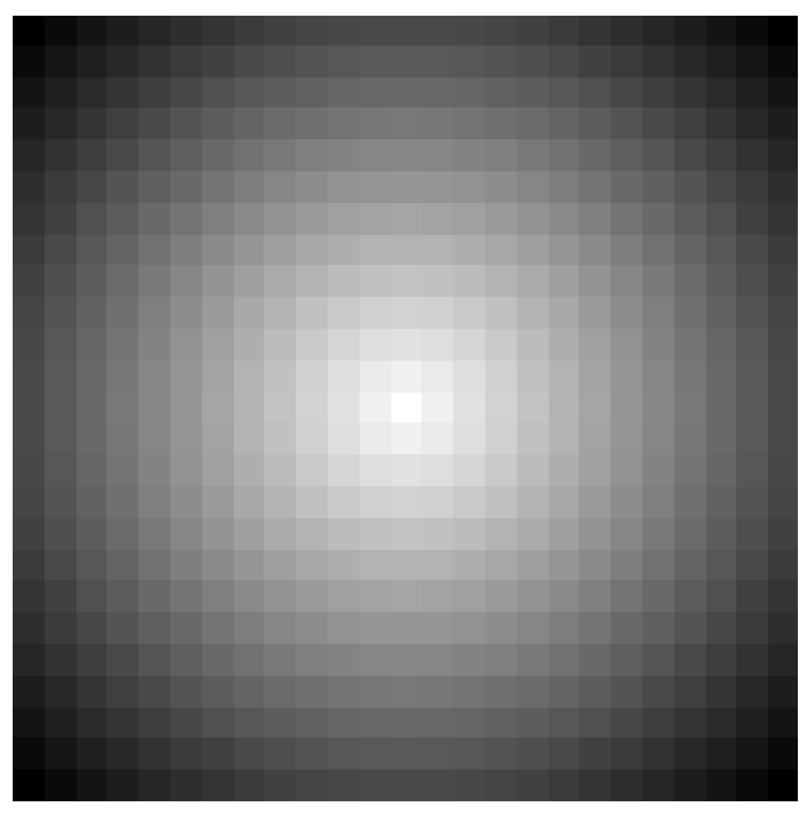
3.2.2. Gradient Mask

The essence of a gradient mask is a weight matrix with the highest value at the center and decreasing values as they move away from the center. The size of the matrix is  s × s , which is the same as the patch size. The label of the patch is determined by the label of the center pixel, so we can infer that the closer to the center of the patch, the more critical the information. The purpose of setting a gradient mask is to reduce the model’s attention to spatial and spectral information at the patch edges and to increase its attention to the key information at the center. It can be said that this is a forced attention transfer method. Specifically, we set the weight of the center to 1 and the weight of the four vertices to 0 and interpolate the other values linearly based on their distance from the center. The weight calculation formula is as Equation (1).
mask i , j = 1 ( i c e n t e r ) 2 + ( j c e n t e r ) 2 2 c e n t e r 2
where  ( i , j )  is the location of element in the gradient mask,  ( c e n t e r , c e n t e r )  is the location of central element, and  c e n t e r = ( s + 1 ) / 2 mask  is the resulting gradient mask.
The resulting mask is displayed as a grayscale image in Figure 2. The gradient mask is multiplied element-wise with patches  P 0  to obtain  P 0 , whereas P1 is not processed with the gradient mask. The specific processing process is multiplication of the mask with the corresponding position element of each layer of the patch to obtain a weighted new patch. This ensures that the input samples of the upper and lower branches have small differences at the center and large differences at the edges. During the training process of contrastive learning, in order to achieve the goal of reducing the loss function of the upper and lower branches, the model gradually reduces its attention to the edges of the patch and focuses more on the key information at the center.

3.3. Contrastive Learning

We put  ( v i , v i )  into the BYOL structure, where  v i  is input to the online network, which is then encoded to obtain the representation  u i = f o n l i n e ( v i ) . The representation  z i = g o n l i n e ( u i )  is then obtained through a projector, and the predicted result  k i = q o n l i n e ( z i )  is obtained through a predictor. On the other hand,  v i  is input to the target network, which is then encoded to obtain  u i = f t a r g e t ( v i ) , and the representation  z i = g t a r g e t ( u i )  is obtained through a projector. Specifically, the encoder consists of three 3D convolutional layers, a convolutional layer, and a fully connected layer. After convolution, the output is flattened and then input to the fully connected layer. Each layer is followed by batch normalization and a ReLU activation function. The projector consists of a fully connected layer, batch normalization, and a ReLU activation function. The predictor is a narrower fully connected layer, also followed by batch normalization and a ReLU activation function.
The computation process of the online and target networks can be represented by Equations (2) and (3). For BYOL, its optimization objective is for the positive examples of the online network to approach the positive examples of the target network in the representation space. Therefore, we update the parameters of the online network using a loss function and update the parameters of the target network using an exponential moving average based on the parameters of the online network, with the update step controlled by the hyperparameter  τ . The loss  L  is calculated based on the outputs of the two branches. First, we perform L2 normalization on  k i  and  z i k ¯ i = k i / k i 2 z ¯ = z i / z i 2  and then take the L2-normalization of their difference, as shown in Equation (4).
k i = q o n l i n e ( g o n l i n e ( f o n l i n e ( v i ) ) )
z i = g t a r g e t ( f t a r g e t ( v i ) )
L = k ¯ i z ¯ 2 2 = 2 2 · k i , z k i · z
As the BYOL structure is asymmetric, in order to fully utilize the data, we exchange the input patches of the two branches, i.e., inputting  v i  to the target network and  v i  to the online network, and calculate the loss function  L . It can also greatly increase the efficiency of optimization. The loss function of BYOL is shown as Equation (5):
L B Y O L = L + L
L B Y O L  is the symmetric loss and we update the parameters according to it. The process of parameter update can be represented as Equations (6) and (7):
W o n l i n e o p t i m i z e r ( W o n l i n e , W o n l i n e L B Y O L , η )
W t a r g e t τ W t a r g e t + ( 1 τ ) W o n l i n e
where  W o n l i n e  is the parameter of the online network, while  W t a r g e t  is the parameter of the target network.  η  is the learning rate and  τ  is the weight of parameter update. ← means assignment.
After reaching the specified number of iterations during training, we save the parameters of the encoder and projector and use the output of the projector as features inputted into the downstream task. In order to evaluate the ability of the contrastive learning model to extract features after introducing UPDA, we use the classical SVM classifier as the downstream task, with classification accuracy as the indicator to evaluate the performance of the features.
We split the sample patches into training and testing sets and use the features of the training set to train the classifier. The features of the test set are input to the trained classifier to obtain the classification result  Y ^ = { y ^ 0 , y ^ 1 , , y ^ N } ( y ^ i N ) . According to  Y ^  and  Y , we calculate the accuracy of every class, the overall accuracy (OA), and the average accuracy (AA).

4. Experiments and Results

In this section, we report some classification experiments based on our method, and provide a detailed analysis of the experimental results.

4.1. Datasets

In the classification experiments, three publicly available datasets are used to show the superior performance of our method UPDA, including the Indian Pines (IP), Pavia University (PU), and Salina (SA) datasets.
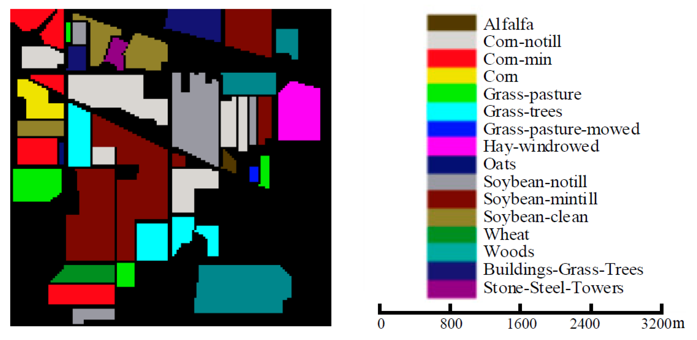
The IP dataset was gathered by the AVIRIS sensor over the Indian Pines test site in northwestern Indiana. It includes 145 × 145 pixels and 224 spectral reflectance bands within the wavelength range of  0.4 2.5 × 10 6  m. After eliminating bands covering water absorption regions, 200 bands remained, and the ground truth was composed of 16 classes. However, the dataset suffers from an uneven sample size issue, with the largest class having over 2000 samples and the smallest class having only 20 samples. Additionally, the dataset has a relatively low spatial resolution, which poses a challenge for classification. For more information on the IP dataset, please refer to Figure 3 and Table 1.
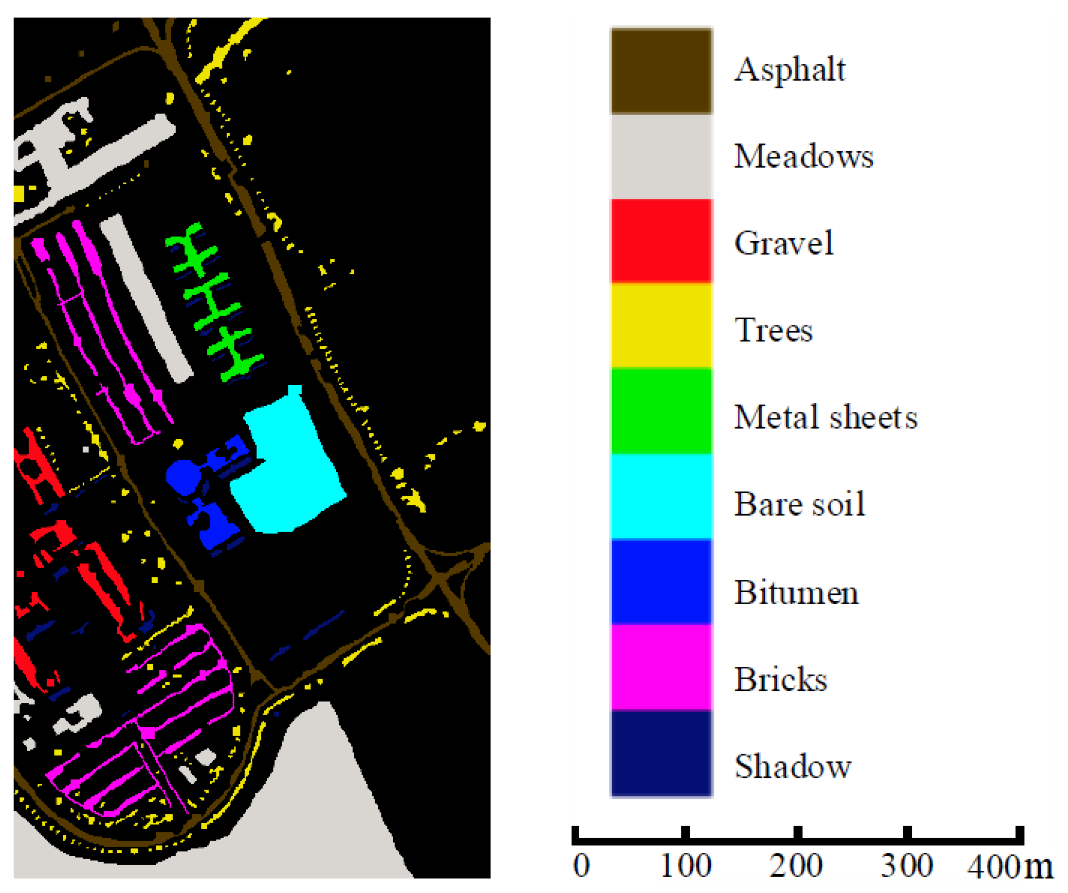
The PU dataset comprises of 610 × 340 pixels and 103 spectral bands within the wavelength range of  0.43 0.86 × 10 6  m. The ground truth is composed of nine classes. This dataset is characterized by complex background pixels, small connected regions, and numerous discontinuous pixels. Moreover, its wavelength range is smaller than the other two datasets, resulting in less spectral information. For more information on the PU dataset, please refer to Figure 4 and Table 2.
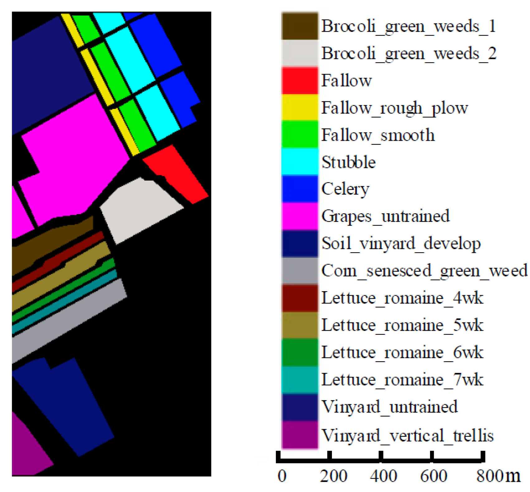
The SA dataset is an image with 512 × 217 pixels and 224 spectral bands within the wavelength range of  0.36 2.5 × 10 6  m. After removing 20 water-absorbing bands, 204 spectral bands remain, and the ground truth is composed of 16 landcover classes. Compared to the other two datasets, the SA dataset is easier to classify due to its fewer obvious flaws such as uneven samples, low resolution, or complex background. For more information on the SA dataset, refer to Figure 5 and Table 3.

4.2. Experimental Settings

We designed the backbone network for contrastive learning based on structure of HybridSN, which consists of 3D convolutional layers, and 2D convolutional layers, and the specific network shape of online network and target network are shown in Table 4.
We set the batch size to 128 and the size of the input patch s, to  25 × 25 . Considering the low spatial resolution and uneven samples of the IP dataset, the principal component maps were taken as the first 30 for the IP dataset and the first 15 for the PU and SA datasets. In training the classifier, all available labeled pixels were divided into training and testing sets, 10% were randomly selected as training sets for the IP and PU datasets, and 5% for the SA dataset. The number of contrastive learning epochs was set to 50. The coefficient of EMA,  τ , was set to 0.99. The selection of the above parameters is partly based on [11,25] and partly verified by experiments.
In order to verify whether the patch size s and the number of principal component graphs d are appropriate, we conducted some verification experiments on the IP and PU dataset. Indeed, when  s = 25  and  d = 30 , the features extracted by BYOL make the classifier to achieve the highest classification accuracy on the IP dataset, while  d = 15  on the PU dataset. The results are shown in Table 5, Table 6 and Table 7.
As for the SVM classifier, we chose “rbf” kernels, the penalty coefficient was set to 10 or 100, and the gamma was set to 0.01 or 0.001. They were obtained through experimental traversal.
The hardware configuration for the experiment was as follows: NVIDIA GeForce GTX 1660 SUPER GPU, Intel Core i7-10700 CPU, and 16 GB DRAM. The software configuration included Windows 10, Python 3.8, Pytorch 1.8.0, and Scikit-learn 0.24.2.
Two well-known metrics were used to evaluate the performance of different methods: accuracy (OA) and average accuracy (AA). All experiments were repeated three times, and the mean values of the results were recorded.

4.3. Classification Performance

To prove the superiority of our method, seven other unsupervised feature extraction methods were adopted as a baseline for comparison: PCA, tensor principal component analysis (TPCA) [36], stacked sparse autoencoder (SSAE) [37], unsupervised deep feature extraction (EPLS) [38], 3D convolutional autoencoder (3DCAE) [39], ContrastNet [40], and basic BYOL [25].
The classification results in the IP dataset are shown in Table 8. Our method obtains the best OA and AA values, and performs the best in 10 classes, particularly in classes 3, 4, 10, 11, 14, and 15. In classes with very few samples such as Alfalfa, Oats and Stone-Steel-Towers, our method leaves some room for improvement, and in classes with small inter-class gaps, “UPDA + BYOL” is good at distinguishing them, such as class Corn-nottill, Corn-mintill, Corn, Grass-pasture, Grass-trees, Grass-pasture-mowed, Soybean-nottill, Soybean-mintill, and Soybean-clean, which belong to different stages of the same crop. The introduction of UPDA increases the OA of BYOL by 2.29%, and increases the AA by 2.84%, which is a giant leap.
The classification results in the PU dataset are shown in Table 9. The OA and AA of our method are the highest and it obtains the best accuracy in six of nine classes. Particularly in classes 1, 2, 3, 6, 7, and 8, “UPDA + BYOL” performs much better than the other methods. Regrettably, in the class shadows “UPDA + BYOL” is not as good as the baselines. We guess that the ground cover of the class shadows is not single and our method tends to divide different material in the same class. In addition, our method outperforms the original BYOL in every class, OA, and AA, which demonstrates the effect of introducing UPDA. Furthermore, the introduction of UPDA increases the OA of BYOL by 1.51% and increases the AA by 3.46%.
The classification results in the SA dataset are shown in Table 10. “UPDA + BYOL” performs the best in OA, AA, and all classes except classes 1, 6, 11, and 12. After introducing UPDA, the OA, AA, and accuracy values in each class are all close to 100%, and the introduction of UPDA increases the OA of BYOL by 0.47% and increases the AA by 0.46%, which demonstrates that our method has excellent performance on ideal datasets.
The time consumption of our method and ContrastNet on three datasets are shown in Table 11. Time consumption of our method is significantly shorter than ContrastNet.
Overall, our method achieves the best results on the three datasets and greatly outperforms other comparative methods.

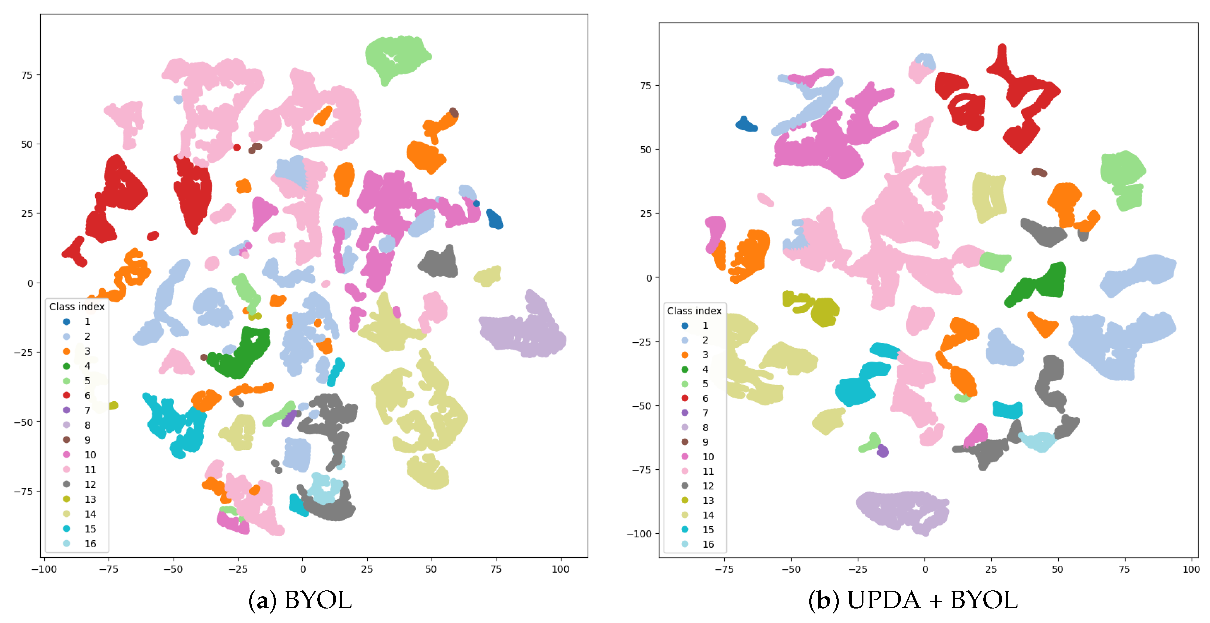
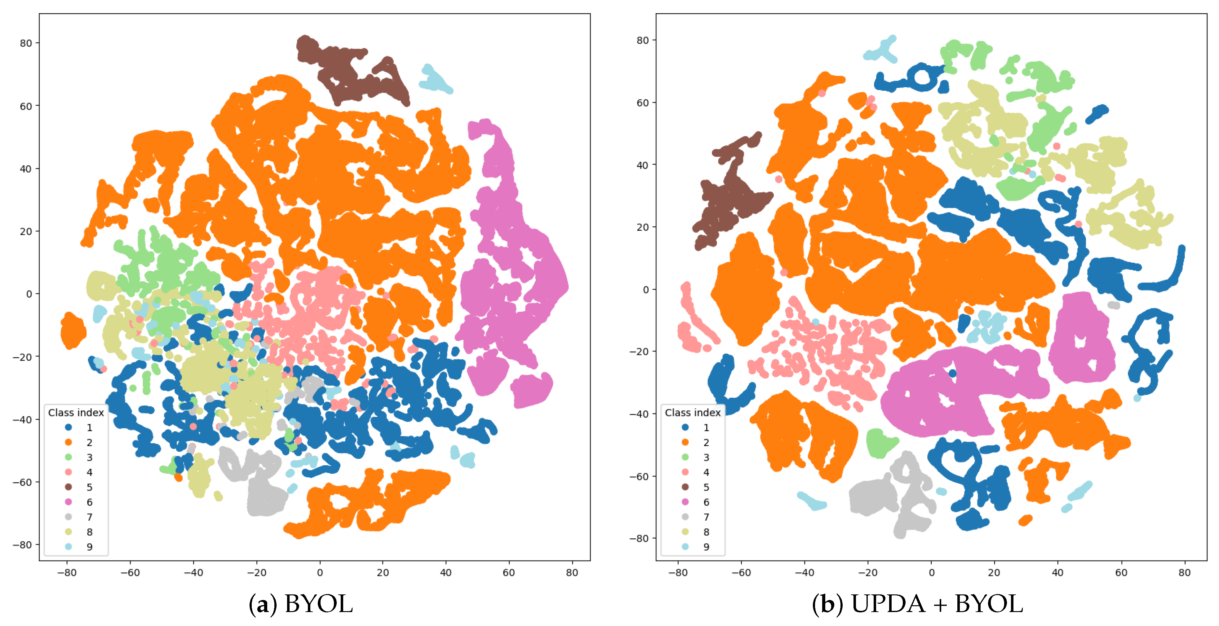
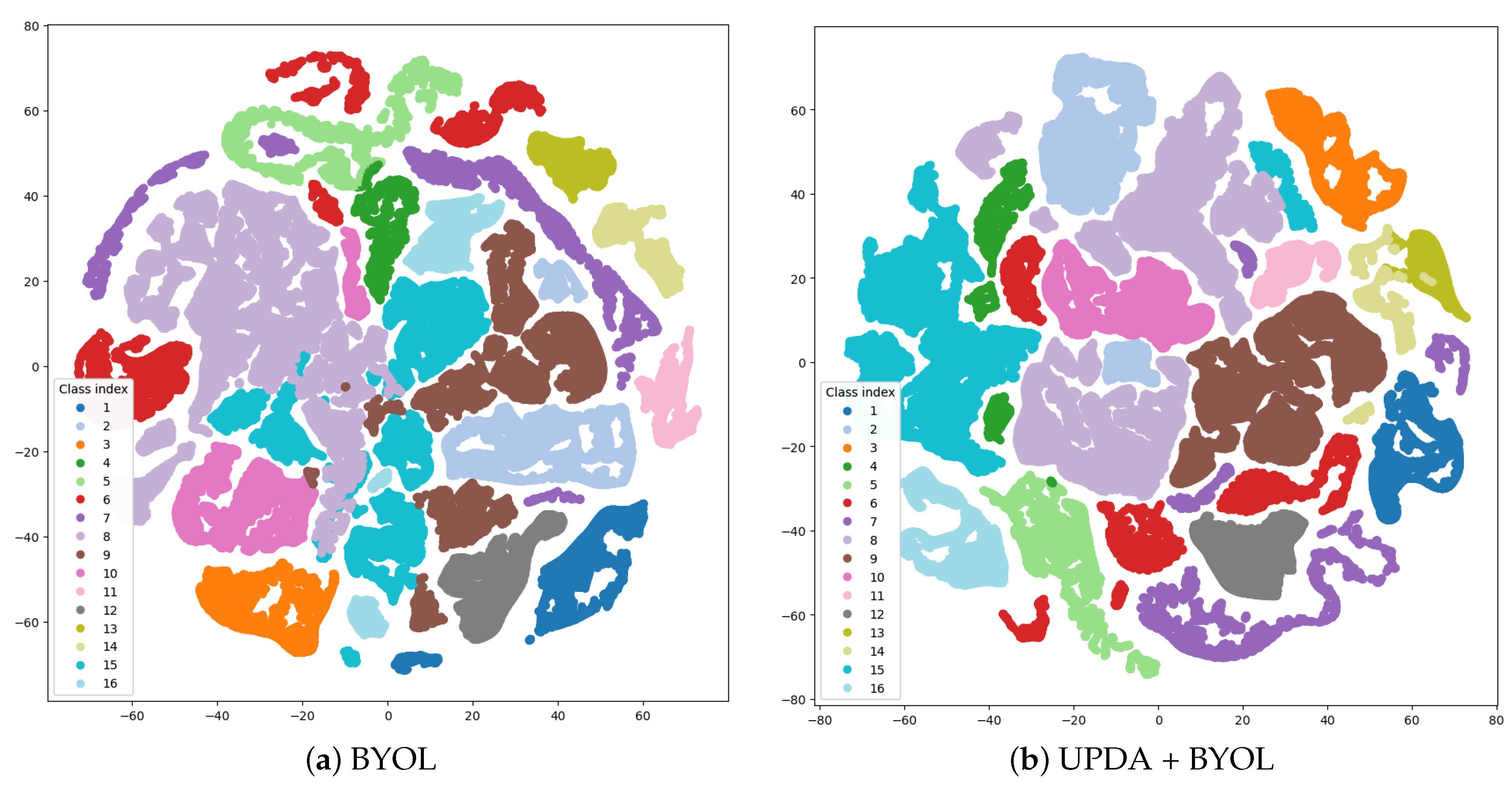
4.4. Feature Visualization

To further assess the effectiveness of UPDA, we utilized the t-distributed stochastic neighbor embedding (t-SNE) [41] method to visualize the learned representation of spatial–spectral features. For comparison, we also visualized the feature extracted by the BYOL without UPDA. The results are presented in Figure 6, Figure 7 and Figure 8.
In the IP dataset, subfigure (b) displays a more concentrated distribution of color blocks belonging to the same class, with fewer fine points, and the shape is more towards blocks than bars. Classes with few samples such as classes 1, 7, and 9 become easier to separate from other classes.
In the PU dataset, the classes 1, 4, 7, 8, and 9 are partly mixed in subfigure (a), but there are fewer overlapping parts of the color blocks in (b), which means that there exists a larger gap between classes. Furthermore, it is obvious that blocks of class 2 and 6 become more tightly connected after introducing UPDA.
In the SA dataset, the pores in the color block of (b) are smaller, and the fine blocks are almost gone. In addition, the contact points between different color blocks are reduced. After introducing UPDA, the features of classes 13 and 14 are glued together, but the features of classes 1, 10, and 15 are obviously more isolated.
By comparing the visualization of features, we can conclude that UPDA can help BYOL to reduce the intra-class gap, increase the inter-class gap, and improve the representation of features.

4.5. Analysis of Different Strategies

In order to investigate the impact of different data augmentation methods in UPDA on classification performance, we conducted ablation experiments. In addition to the blank group and the complete group, we created the “BE”, “RO”, “GM”, “BE + RO”, “BE + GM”, and “RO + GM” groups, and conducted experiments on three datasets. We repeated each experiment three times and recorded the average OA.
Table 12 shows the results. The “BE + GM + RO” group achieved the best OA in all three datasets, which shows that the combination of the three strategies is most effective.
The “BE + GM” group achieved second place in the IP and SA dataset and third place in the PU dataset. The “GM + RO” group achieved second place in the PU dataset and third place in the SA dataset. In general, when the strategies are grouped in pairs, the effect varies according to different datasets.
When each strategy is joined individually, RO performs better than GM and BE, and BE performs the worst overall. There is no doubt that the introduction of each strategy improves the results, and they achieve the best classification performance when working together.
When considering the characteristics of the dataset, we can also analyze the strengths and weaknesses of each strategy. For the PU datasets with a small wavelength range and complex background, the effect of RO is the most significant and the effect of BE is the weakest when compared with other datasets. We can infer that RO can help to more effectively extract spatial features from environments where spatial features are not obvious, and BE can work better in datasets rich in spectral information. The performances of GM in different datasets are quite varied, and it is less pronounced when combined with other strategies.

5. Conclusions

This letter introduces a novel and efficacious approach, UPDA, which aims to bolster the performance of contrastive learning in HSIC. The approach is designed to enhance the representation of spatial–spectral features through a series of predominant data augmentation strategies designed for HSIs. By utilizing our method to extract features from a vast amount of data in an unsupervised manner and subsequently training a classifier with a small number of labels, exceptional classification accuracy can be achieved. The experimental results evidence the superiority of our method, and the ablation study underscores the effectiveness and distinctions of each strategy. Our method is highly adaptable, allowing for the incorporation of new strategies, and has tremendous potential to enhance the ability of contrastive learning, leading to better results with fewer labels. Furthermore, UPDA is not only applicable to BYOL but can also unlock the potential of other contrastive learning methods. We anticipate that our work will inspire novel ideas in fellow researchers and facilitate the more effective application of contrastive learning in the field of HSI.

Author Contributions

Methodology, J.L.; Software, J.L.; Formal analysis, J.L. and X.L.; Resources, X.L. and Y.Y.; Writing—original draft, J.L.; Writing—review & editing, J.L.; Visualization, J.L.; Funding acquisition, X.L. and Y.Y. All authors have read and agreed to the published version of the manuscript.

Funding

The research was funded by the National Nature Science Foundation of China under Grant No. 62171404, and in part by the Joint Fund Project of Chinese Ministry of Education under Grant No. 8091B022118.

Data Availability Statement

The data presented in this study are available on http://www.ehu.eus/ccwintco/index.php/Hyperspectral_Remote_Sensing_Scenes.

Conflicts of Interest

The authors declare no conflict of interest.

Abbreviations

The following abbreviations are used in this manuscript:
HSIHyperspectral image
HSICHyperspectral image classification
UPDAUnlock the potential of data augmentation
BYOLBootstrap your own latent
PCAPrincipal component analysis
ICAIndependent component analysis
LDALinear discriminant analysis
MDSMultidimensional scaling
CNNConvolutional neural network
DRNNDeep recurrent neural network
DFFNDeep feed-forward networks
AEAutoencoder
GANGenerative adversarial network
AAEAdversarial autoencoder
VAEVariational autoencoder
MAEMasked autoencoder
DCGANDeep convolutional generative adversarial network
InfoGANInformation-maximizing generative adversarial network
MocoMomentum contrast
SimCLRA simple framework for contrastive learning of visual representations
SimSiamSimple Siamese
BEBand erasure
RORandom occlusion
GMGradient mask
OAOverall accuracy
AAAverage accuracy
IPIndian pines
PUUniversity of Pavia
SASalina
EMAExponential moving average
TPCATensor principal component analysis
SSAEStacked sparse autoencoder
EPLSUnsupervised deep feature extraction
3DCAE3 dimensional convolutional autoencoder

References

  1. Datta, D.; Mallick, P.K.; Bhoi, A.K.; Ijaz, M.F.; Shafi, J.; Choi, J. Hyperspectral image classification: Potentials, challenges, and future directions. Comput. Intell. Neurosci. 2022, 2022, 3854635. [Google Scholar] [CrossRef] [PubMed]
  2. Stuart, M.B.; McGonigle, A.J.; Willmott, J.R. Hyperspectral imaging in environmental monitoring: A review of recent developments and technological advances in compact field deployable systems. Sensors 2019, 19, 3071. [Google Scholar] [CrossRef] [PubMed] [Green Version]
  3. Tong, X.; Xie, H.; Weng, Q. Urban land cover classification with airborne hyperspectral data: What features to use? IEEE J. Sel. Top. Appl. Earth Obs. Remote. Sens. 2013, 7, 3998–4009. [Google Scholar] [CrossRef]
  4. Duan, P.; Ghamisi, P.; Kang, X.; Rasti, B.; Li, S.; Gloaguen, R. Fusion of Dual Spatial Information for Hyperspectral Image Classification. IEEE Trans. Geosci. Remote. Sens. 2021, 59, 7726–7738. [Google Scholar] [CrossRef]
  5. Wold, S.; Esbensen, K.; Geladi, P. Principal component analysis. Chemom. Intell. Lab. Syst. 1987, 2, 37–52. [Google Scholar] [CrossRef]
  6. Villa, A.; Benediktsson, J.A.; Chanussot, J.; Jutten, C. Hyperspectral image classification with independent component discriminant analysis. IEEE Trans. Geosci. Remote. Sens. 2011, 49, 4865–4876. [Google Scholar] [CrossRef] [Green Version]
  7. Du, Q. Modified Fisher’s linear discriminant analysis for hyperspectral imagery. IEEE Geosci. Remote. Sens. Lett. 2007, 4, 503–507. [Google Scholar] [CrossRef]
  8. Kruskal, J.B.; Wish, M.; Uslaner, E.M. Multidimensional scaling. In Handbook of Perception and Cognition; Academic Press: Cambridge, MA, USA, 1978. [Google Scholar]
  9. Hu, W.; Huang, Y.; Wei, L.; Zhang, F.; Li, H. Deep convolutional neural networks for hyperspectral image classification. J. Sensors 2015, 2015, 258619. [Google Scholar] [CrossRef] [Green Version]
  10. Chen, Y.; Jiang, H.; Li, C.; Jia, X.; Ghamisi, P. Deep feature extraction and classification of hyperspectral images based on convolutional neural networks. IEEE Trans. Geosci. Remote. Sens. 2016, 54, 6232–6251. [Google Scholar] [CrossRef] [Green Version]
  11. Roy, S.K.; Krishna, G.; Dubey, S.R.; Chaudhuri, B.B. HybridSN: Exploring 3D-2D CNN Feature Hierarchy for Hyperspectral Image Classification. IEEE Geosci. Remote. Sens. Lett. 2020, 17, 277–281. [Google Scholar] [CrossRef] [Green Version]
  12. Zhong, Z.; Li, J.; Luo, Z.; Chapman, M. Spectral–spatial residual network for hyperspectral image classification: A 3-D deep learning framework. IEEE Trans. Geosci. Remote. Sens. 2017, 56, 847–858. [Google Scholar] [CrossRef]
  13. Hang, R.; Li, Z.; Liu, Q.; Ghamisi, P.; Bhattacharyya, S.S. Hyperspectral image classification with attention-aided CNNs. IEEE Trans. Geosci. Remote. Sens. 2020, 59, 2281–2293. [Google Scholar] [CrossRef]
  14. Zhang, X.; Sun, Y.; Jiang, K.; Li, C.; Jiao, L.; Zhou, H. Spatial sequential recurrent neural network for hyperspectral image classification. IEEE J. Sel. Top. Appl. Earth Obs. Remote. Sens. 2018, 11, 4141–4155. [Google Scholar] [CrossRef] [Green Version]
  15. Ballard, D.H. Modular Learning in Neural Networks. In Proceedings of the 6th National Conference on Artificial Intelligence (AAAI-87), Seattle, WA, USA, 13–17 July 1987; pp. 279–284. [Google Scholar]
  16. Goodfellow, I.; Pouget-Abadie, J.; Mirza, M.; Xu, B.; Warde-Farley, D.; Ozair, S.; Courville, A.; Bengio, Y. Generative adversarial nets. In Proceedings of the 28th Conference on Neural Information Processing Systems, Montreal, QC, Canada, 8–13 December 2014; pp. 2672–2680. [Google Scholar]
  17. Makhzani, A.; Shlens, J.; Jaitly, N.; Goodfellow, I.; Frey, B. Adversarial autoencoders. arXiv 2015, arXiv:1511.05644. [Google Scholar]
  18. Kingma, D.P.; Welling, M. Auto-encoding variational bayes. arXiv 2013, arXiv:1312.6114. [Google Scholar]
  19. He, K.; Chen, X.; Xie, S.; Li, Y.; Dollár, P.; Girshick, R. Masked autoencoders are scalable vision learners. In Proceedings of the IEEE/CVF Conference on Computer Vision and Pattern Recognition, New Orleans, LA, USA, 19–24 June 2022; pp. 16000–16009. [Google Scholar]
  20. Radford, A.; Metz, L.; Chintala, S. Unsupervised representation learning with deep convolutional generative adversarial networks. arXiv 2015, arXiv:1511.06434. [Google Scholar]
  21. Chen, X.; Duan, Y.; Houthooft, R.; Schulman, J.; Sutskever, I.; Abbeel, P. Infogan: Interpretable representation learning by information maximizing generative adversarial nets. In Proceedings of the 30th Conference on Neural Information Processing Systems, Barcelona, Spain, 5–10 December 2016; Volume 29. [Google Scholar]
  22. Hang, R.; Zhou, F.; Liu, Q.; Ghamisi, P. Classification of hyperspectral images via multitask generative adversarial networks. IEEE Trans. Geosci. Remote. Sens. 2020, 59, 1424–1436. [Google Scholar] [CrossRef]
  23. He, K.; Fan, H.; Wu, Y.; Xie, S.; Girshick, R. Momentum Contrast for Unsupervised Visual Representation Learning. In Proceedings of the The IEEE/CVF Conference on Computer Vision and Pattern Recognition (CVPR), Online, 16–18 June 2020. [Google Scholar]
  24. Chen, T.; Kornblith, S.; Norouzi, M.; Hinton, G. A simple framework for contrastive learning of visual representations. In Proceedings of the 37th International Conference on Machine Learning (PMLR), Vienna, Austria, 12–18 July 2020; pp. 1597–1607. [Google Scholar]
  25. Grill, J.B.; Strub, F.; Altché, F.; Tallec, C.; Richemond, P.; Buchatskaya, E.; Doersch, C.; Avila Pires, B.; Guo, Z.; Gheshlaghi Azar, M.; et al. Bootstrap your own latent-a new approach to self-supervised learning. In Proceedings of the 34th Conference on Neural Information Processing Systems, Online, 6–12 December 2020; Volume 33, pp. 21271–21284. [Google Scholar]
  26. Caron, M.; Misra, I.; Mairal, J.; Goyal, P.; Bojanowski, P.; Joulin, A. Unsupervised learning of visual features by contrasting cluster assignments. In Proceedings of the 34th Conference on Neural Information Processing Systems, Online, 6–12 December 2020; Volume 33, pp. 9912–9924. [Google Scholar]
  27. Chen, X.; He, K. Exploring simple siamese representation learning. In Proceedings of the IEEE/CVF Conference on Computer Vision and Pattern Recognition, Online, 19–25 June 2021; pp. 15750–15758. [Google Scholar]
  28. Hang, R.; Qian, X.; Liu, Q. Cross-Modality Contrastive Learning for Hyperspectral Image Classification. IEEE Trans. Geosci. Remote. Sens. 2022, 60, 5532812. [Google Scholar] [CrossRef]
  29. Guan, P.; Lam, E.Y. Cross-domain contrastive learning for hyperspectral image classification. IEEE Trans. Geosci. Remote. Sens. 2022, 60, 5528913. [Google Scholar] [CrossRef]
  30. Shu, Z.; Liu, Z.; Zhou, J.; Tang, S.; Yu, Z.; Wu, X.J. Spatial–Spectral Split Attention Residual Network for Hyperspectral Image Classification. IEEE J. Sel. Top. Appl. Earth Obs. Remote. Sens. 2022, 16, 419–430. [Google Scholar] [CrossRef]
  31. Haut, J.M.; Paoletti, M.E.; Plaza, J.; Plaza, A.; Li, J. Hyperspectral Image Classification Using Random Occlusion Data Augmentation. IEEE Geosci. Remote. Sens. Lett. 2019, 16, 1751–1755. [Google Scholar] [CrossRef]
  32. Halvagal, M.S.; Laborieux, A.; Zenke, F. Predictor networks and stop-grads provide implicit variance regularization in BYOL/SimSiam. arXiv 2022, arXiv:2212.04858. [Google Scholar]
  33. Ding, K.; Xu, Z.; Tong, H.; Liu, H. Data augmentation for deep graph learning: A survey. ACM SIGKDD Explor. Newsl. 2022, 24, 61–77. [Google Scholar] [CrossRef]
  34. Xiao, T.; Wang, X.; Efros, A.A.; Darrell, T. What should not be contrastive in contrastive learning. arXiv 2020, arXiv:2008.05659. [Google Scholar]
  35. Li, J.; Li, X.; Cao, Z.; Zhao, L. ROBYOL: Random-Occlusion-Based BYOL for Hyperspectral Image Classification. IEEE Geosci. Remote. Sens. Lett. 2022, 19, 6014405. [Google Scholar] [CrossRef]
  36. Ren, Y.; Liao, L.; Maybank, S.J.; Zhang, Y.; Liu, X. Hyperspectral image spectral-spatial feature extraction via tensor principal component analysis. IEEE Geosci. Remote. Sens. Lett. 2017, 14, 1431–1435. [Google Scholar] [CrossRef] [Green Version]
  37. Tao, C.; Pan, H.; Li, Y.; Zou, Z. Unsupervised spectral–spatial feature learning with stacked sparse autoencoder for hyperspectral imagery classification. IEEE Geosci. Remote. Sens. Lett. 2015, 12, 2438–2442. [Google Scholar]
  38. Romero, A.; Gatta, C.; Camps-Valls, G. Unsupervised deep feature extraction for remote sensing image classification. IEEE Trans. Geosci. Remote. Sens. 2015, 54, 1349–1362. [Google Scholar] [CrossRef] [Green Version]
  39. Mei, S.; Ji, J.; Geng, Y.; Zhang, Z.; Li, X.; Du, Q. Unsupervised Spatial–Spectral Feature Learning by 3D Convolutional Autoencoder for Hyperspectral Classification. IEEE Trans. Geosci. Remote. Sens. 2019, 57, 6808–6820. [Google Scholar] [CrossRef]
  40. Cao, Z.; Li, X.; Feng, Y.; Chen, S.; Xia, C.; Zhao, L. ContrastNet: Unsupervised feature learning by autoencoder and prototypical contrastive learning for hyperspectral imagery classification. Neurocomputing 2021, 460, 71–83. [Google Scholar] [CrossRef]
  41. Van der Maaten, L.; Hinton, G. Visualizing data using t-SNE. J. Mach. Learn. Res. 2008, 9, 2579–2605. [Google Scholar]
Figure 1. The framework of our method (UPDA + BYOL). The original dataset is band erased to obtain the data of the two branches. After PCA and sliding window segmentation, two series of patch groups are obtained. A pair of patches is used as an example in the figure. Gradient mask is applied to the patch of upper branch, and two views are obtained. Two views are regarded as a pair of positive samples and put into the backbone network of BYOL. SG denotes the stop gradient. After training, the features are saved to train the SVM classifier.
Remotesensing 15 03123 g001
Figure 2. Visualization of the Gradient Mask.
Remotesensing 15 03123 g002
Figure 3. Groundtruth of the IP dataset.
Remotesensing 15 03123 g003
Figure 4. Groundtruth of the PU dataset.
Remotesensing 15 03123 g004
Figure 5. Groundtruth of the SA dataset.
Remotesensing 15 03123 g005
Figure 6. Visualization of extracted features in the Indian Pines dataset.
Remotesensing 15 03123 g006
Figure 7. Visualization of extracted features in the University of Pavia dataset.
Remotesensing 15 03123 g007
Figure 8. Visualization of extracted features in the Salinas dataset.
Remotesensing 15 03123 g008
Table 1. Details of the IP dataset.
IP Dataset
Class NameNo.NumberTraining
Alfalfa1465
Corn-notill21428143
Corn-mintill383083
Corn423724
Grass-pasture548348
Grass-trees67302
Grass-pasture-mowed7283
Hay-windrowed847848
Oats9202
Soybean-notill1097297
Soybean-mintill112455246
Soybean-clean1259359
Wheat1320521
Woods141265127
Buildings-Grass-Trees-Drives1538639
Stone-Steel-Towers16939
Total 10,249
Table 2. Details of the PU dataset.
PU Dataset
Class NameNo.NumberTraining
Asphalt16631663
Meadows218,6491865
Gravel32099210
Trees43064306
Painted metal sheets51345135
Bare Soil65029503
Bitumen71330133
Self-Blocking Bricks83682368
Shadows994795
Total 42,776
Table 3. Details of the SA dataset.
SA Dataset
Class NameNo.NumberTraining
Brocoli_green_weeds_112009100
Brocoli_green_weeds_223726186
Fallow3197699
Fallow_rough_plow4139470
Fallow_smooth52678134
Stubble63959198
Celery73579179
Grapes_untrained811,271564
Soil_vinyard_develop96203310
Corn_senesced_green_weeds103278164
Lettuce_romaine_4wk11106853
Lettuce_romaine_5wk12192796
Lettuce_romaine_6wk1391646
Lettuce_romaine_7wk14107054
Vinyard_untrained157268363
Vinyard_vertical_trellis16180790
Total 54,129
Table 4. Structure of backbone network. The output shape of each layer is defined in PyTorch style. Batch size in the shape array is denoted by −1.
Layer TypeOnline NetworkTarget Network
input[−1,1,15/30,25,25][−1,1,15/30,25,25]
Conv3d[−1,8,7,23,23][−1,8,7,23,23]
BatchNorm3d[−1,8,7,23,23][−1,8,7,23,23]
ReLU[−1,8,7,23,23][−1,8,7,23,23]
Conv3d[−1,16,5,21,21][−1,16,5,21,21]
BatchNorm3d[−1,16,5,21,21][−1,16,5,21,21]
ReLU[−1,16,5,21,21][−1,16,5,21,21]
Conv3d[−1,32,3,19,19][−1,32,3,19,19]
BatchNorm3d[−1,32,3,19,19][−1,32,3,19,19]
ReLU[−1,32,3,19,19][−1,32,3,19,19]
Conv2d[−1,64,17,17][−1,64,17,17]
BatchNorm2d[−1,64,17,17][−1,64,17,17]
ReLU[−1,64,17,17][−1,64,17,17]
Linear[−1,1024][−1,1024]
ReLU[−1,1024][−1,1024]
Linear[−1,128][−1,128]
ReLU[−1,16]/
Linear[−1,16]/
Table 5. Comparison of different patch sizes s in the IP dataset, setting d as 30, introducing only RO.
s21232527
OA (%)93.8695.0396.6196.21
Table 6. Comparison of different number of principal component graphs d in the IP dataset, setting s as 25, introducing only RO.
d15202530
OA (%)95.1196.0095.9496.61
Table 7. Comparison of different number of principal component graphs d in the PU dataset, setting s as 25, introducing only RO.
d13151720
OA (%)97.9898.4097.4697.35
Table 8. Comparison in the Indian Pines dataset. 10% labeled samples were used for training, and the rest were used for testing. The highest accuracy values in every row are in bold. Some of the data in the table are quoted from [39].
No.ClassPCATPCASSAEEPLS3DCAEContrastNetBYOLUPDA + BYOL
1Alfalfa39.0260.9756.2558.7290.4885.3792.6890.24
2Corn-notill72.3087.0069.5859.9192.4997.1594.4295.33
3Corn-mintill72.0294.5175.3671.3490.3797.9594.4298.26
4Corn55.8779.3464.5874.3186.9095.6292.6497.34
5Grass-pasture93.0993.0888.8197.9594.2596.0997.0198.85
6Grass-trees94.6796.3487.0096.4497.0796.8098.2298.78
7Grass-pasture-mowed80.0076.0090.0054.0291.2670.6798.67100.00
8Hay-windrowed98.3799.7689.7288.9997.7998.6899.5399.30
9Oats88.89100.00100.0058.8975.9170.3775.9383.33
10Soybean-nottill74.4979.5177.1973.1087.3497.4594.3698.06
11Soybean-mintill69.5885.4277.5870.7890.2498.4097.4799.17
12Soybean-clean65.2984.2472.0057.5195.7693.5788.0196.25
13Wheat98.3798.9187.8099.2597.4995.3297.3096.22
14Woods91.3998.0693.4895.0796.0398.5198.3999.71
15Buildings-Grass-Trees-Drives48.9987.3172.3691.2690.4896.7394.5298.66
16Stone-Steel-Towers87.9596.3897.2291.2798.8279.7675.4084.92
AA (%)76.8989.3181.1877.4392.0491.7893.0695.90
OA (%)76.8888.5579.7877.1892.3597.0895.7198.00
Table 9. Comparison in the University of Pavia dataset. A total of 10% labeled samples were used for training, and the rest were used for testing. The highest accuracy in every row are in bold. Some of the data in the table are quoted from [39].
No.ClassPCATPCASSAEEPLS3DCAEContrastNetBYOLUPDA + BYOL
1Asphalt90.8996.1795.7295.9595.2199.4998.2199.94
2Meadows93.2797.9594.1395.9196.0699.9899.6299.99
3Gravel82.6086.5087.4794.3391.3299.0695.1599.17
4Trees92.4194.8496.9199.2898.2897.7596.4199.27
5Painted metal sheets98.98100.0099.7699.9295.5599.8198.2799.78
6Bare Soil92.0094.7695.7693.5795.3099.9099.98100.00
7Bitumen85.8391.8991.1898.1795.1499.8396.1899.89
8Self-Blocking Bricks82.9689.0482.4791.2391.3898.7995.1298.75
9Shadows100.0098.94100.0099.7899.9694.8480.7994.09
AA (%)90.9995.6493.7196.3395.3698.8395.5398.99
OA (%)91.3794.4593.5195.1395.3999.4698.0499.65
Table 10. Comparison in the Salinas dataset. Five percent of the labeled samples were used for training, and the rest were used for testing. The highest accuracy value in every row is in bold. Some of the data in the table are quoted from [39].
No.ClassPCATPCASSAEEPLS3DCAEContrastNetBYOLUPDA + BYOL
0Brocoli_green_weeds_197.4899.88100.0099.99100.0099.9398.3699.95
1Brocoli_green_weeds_299.5299.4999.5299.9299.2999.8099.99100.00
2Fallow99.4199.0494.2498.7597.1399.9599.95100.00
3Fallow_rough_plow99.7799.8499.1798.5297.9198.0199.1999.82
4Fallow_smooth98.7098.9698.8298.3398.2699.4898.9999.92
5Stubble99.6599.80100.0099.9299.9899.9499.9999.97
6Celery99.9499.8499.9497.6999.6499.7999.6199.99
7Grapes_untrained83.9084.1180.7378.8691.5899.5399.3299.93
8Soil_vinyard_develop99.9799.6099.4799.5499.2899.7199.85100.00
9Corn_senesced_green_weeds96.8995.7692.1295.9896.6599.8099.95100.00
10Lettuce_romaine_4wk96.8496.1496.6298.6097.7499.8099.1599.67
11Lettuce_romaine_5wk99.9599.0797.7599.4498.8499.9899.5399.95
12Lettuce_romaine_6w99.54100.0095.8198.8599.2698.20100.00100.00
13Lettuce_romaine_7wk97.2495.7496.6598.5697.4998.6298.7299.74
14Vinyard_untrained76.6879.5479.7383.1387.8599.5398.9899.90
15Vinyard_vertical_trellis97.9098.4099.1299.5098.3499.57100.00100.00
AA (%)96.4693.2495.6196.5597.4599.4899.4799.93
OA (%)92.8796.5792.1192.3595.8199.6099.4899.95
Table 11. Comparison of different methods’ time consumption.
MethodTime Consumption(s)
IPPUSA
ContrastNet2048.923778.734651.70
UPDA + BYOL1545.262544.023214.00
Table 12. The results of the ablation study. Ten percent of the labeled samples were used for training in the IP and PU datasets, and 5% were used in the SA dataset. In every dataset, the three highest OAs are in bold and marked by rank in the lower-right corner.
Group Strategy OA(%)
-BEROGMIPPUSA
(a) 95.7198.0499.48
(b) 96.8198.7799.50
(c) 97.0999.2999.86
(d) 96.1498.9199.64
(e)   97 . 95 2   99 . 60 3   99 . 90 2
(f) 96.9698.9099.69
(g)   97 . 38 3   99 . 64 2   99 . 87 3
(h)   98 . 00 1   99 . 65 1   99 . 95 1
Disclaimer/Publisher’s Note: The statements, opinions and data contained in all publications are solely those of the individual author(s) and contributor(s) and not of MDPI and/or the editor(s). MDPI and/or the editor(s) disclaim responsibility for any injury to people or property resulting from any ideas, methods, instructions or products referred to in the content.

