Article

MSAFNet: Multiscale Successive Attention Fusion Network for Water Body Extraction of Remote Sensing Images

1
College of Computer and Information, Hohai University, Nanjing 211100, China
2
Key Laboratory of Water Big Data Technology of Ministry of Water Resources, Hohai University, Nanjing 211100, China
*
Author to whom correspondence should be addressed.
Remote Sens. 2023, 15(12), 3121; https://doi.org/10.3390/rs15123121
Submission received: 29 May 2023 / Revised: 9 June 2023 / Accepted: 10 June 2023 / Published: 15 June 2023

Abstract

:
Water body extraction is a typical task in the semantic segmentation of remote sensing images (RSIs). Deep convolutional neural networks (DCNNs) outperform traditional methods in mining visual features; however, due to the inherent convolutional mechanism of the network, spatial details and abstract semantic representations at different levels are difficult to capture accurately at the same time, and then the extraction results decline to become suboptimal, especially on narrow areas and boundaries. To address the above-mentioned problem, a multiscale successive attention fusion network, named MSAFNet, is proposed to efficiently aggregate the multiscale features from two aspects. A successive attention fusion module (SAFM) is first devised to extract multiscale and fine-grained features of water bodies, while a joint attention module (JAM) is proposed to further mine salient semantic information by jointly modeling contextual dependencies. Furthermore, the multi-level features extracted by the above-mentioned modules are aggregated by a feature fusion module (FFM) so that the edges of water bodies are well mapped, directly improving the segmentation of various water bodies. Extensive experiments were conducted on the Qinghai-Tibet Plateau Lake (QTPL) and the Land-cOVEr Domain Adaptive semantic segmentation (LoveDA) datasets. Numerically, MSAFNet reached the highest accuracy on both QTPL and LoveDA datasets, including Kappa, MIoU, FWIoU, F1, and OA, outperforming several mainstream methods. Regarding the QTPL dataset, MSAFNet peaked at 99.14% and 98.97% in terms of F1 and OA. Although the LoveDA dataset is more challenging, MSAFNet retained the best performance, with F1 and OA being 97.69% and 95.87%. Additionally, visual inspections exhibited consistency with numerical evaluations.

1. Introduction

With the development of technical aeronautics and space, the coverage of remote sensing images (RSIs) is expanding and the spatial resolution is becoming finer. Since they contain rich ground information that can give detailed feedback on the ground reality, RSIs are widely used in related fields, such as urban planning [1,2,3], agriculture [4], and maritime safety [5]. In hydraulic remote sensing research, accurate water body extraction is crucial for the dynamic monitoring of surface water bodies, surface water level changes [6,7,8], and post-flood damage assessment [9]. First of all, water bodies are characterized by multiple scales and shapes, varying greatly in spatial and geometric scales, which influences the extraction results. Moreover, their spectral information in RSIs is complex [10] and susceptible to interference from glaciers, clouds, and shadows. In summary, mapping water body boundaries accurately can be difficult, which may limit the accuracy of water body extraction. The aim of this research was to improve the water body extraction accuracy from RSIs without making the model overly complex. This was realized by using multi-level feature aggregation and an attention mechanism to extract multiscale water body information.
Two representative methods, the threshold method [11] and the classifier method [12], have been widely used for water body extraction from RSIs. Although simple and easy to implement, the threshold method is more suitable for identifying water bodies with flat terrain and relatively wide water areas. The classifier method improves the accuracy in specific areas but requires human–machine interaction. Overall, these traditional methods are inadequate for handling remote sensing big data.
Deep learning technology is now commonly utilized for image processing after significant advancements in the field. Convolutional neural networks (CNNs) can capture features and assign classification labels to each pixel based on the feature information, because of their powerful feature representation and data-fitting capabilities [13]. As a pioneering design for semantic segmentation, fully convolutional neural networks (FCNs) are extended to allow pixel-level image classification for input images of any size [14]. Continuous convolutional and pooling operations are employed in FCNs to capture deeper semantic information, which also makes them less sensitive to details and leads to the loss of features. To address the problem mentioned, some classical semantic segmentation models and methods have been proposed. UNet, presented in 2015, uses skip connections for the fusion of multiscale feature maps, which has become a foundational network for medical picture segmentation [15]. However, it excessively increases the computational complexity and provides limited improvement in segmentation accuracy. The PSPNet builds the pyramid pooling module to merge the contextual information [16]. Similarly, Chen’s proposed DeepLabV3+ couples an encoder–decoder structure with the ASPP module to alleviate the limitation of receptive fields [17].
RSIs always carry intrinsic correlations between visual properties and implicit semantics, which are essential for identifying multiscale and multi-shape water bodies. Due to inherent complex spectral and spatial information, semantic segmentation methods for natural images provide a limited contribution to the segmentation accuracy of RSIs. Chen et al. raised an adaptive simple linear iterative clustering algorithm to extract high-quality super-pixels from RSIs, followed by a feature decoder to extract water bodies [18]. Isikdogan created a fully convolutional surface water segmentation model called DeepWaterMap based on an encoder–decoder framework to resist noise and useless information, resulting in the desired performance [19]. A separable residual SegNet was proposed by Weng et al. to extract more informative features [20]; similarly, Wang et al. devised residual convolution in the decoder stage to extract multi-level features, which addresses the issue of variation in lake water bodies [21]. Xia et al., investigated a dense skip-connected network called DAU-Net to improve segmentation accuracy in edge regions, which reduces semantic differences by multiscale feature fusion [22]. It is obvious that the mentioned methods are not efficient in extracting multiscale semantic features from RSIs due to inherent complex spectral and spatial information. To address this problem, attention modules are used to promote the fusion of salient features. Attention modules on different dimensions are integrated into SCAttNet, which can select features adaptively, indicating the potential of the attention mechanism to be applied to the semantic segmentation of RSIs [23]. To alleviate the blurred boundary segmentation, Miao proposed edge weighting loss to sharpen the boundary representations [24], and Xu et al., presented a boundary-aware module and a special boundary loss function to extract clearer boundary features [25]. Similarly, Sun proposed a semantic segmentation model with a parallel two-branch structure, which extracts multiscale features from coarse to fine at different levels by a successive pooling operation [26]. SBANet employs a boundary attention module (BA-module) for capturing essential boundary representations by introducing a semantic score from advanced features [27]. To achieve better segmentation results, strong class-constrained features can be mined by the image class feature library and the attention mechanism, proposed by Deng et al. [28]. Li et al., created two modules, DLCAM and SLSAM, to refine and aggregate features at different levels in a dual-attention approach [29]. Liu organically coupled the attention mechanism with a residual structure into the ASPP module, further improving its ability to capture salient features at different scales [30]. However, this approach also leads to an increase in computational complexity. Additionally, attention mechanisms have been applied in hyperspectral image classification (HSIC) [31], and they can extract the spectral information of water bodies in RSIs.
Due to the various scales and shapes, existing methods cannot adequately segment water bodies from RSIs. Attempting to mine and leverage multi-level features to strengthen the semantic distinguishability, a multiscale successive attention fusion network, called MSAFNet, is proposed, which combines multi-level feature aggregation and attention mechanisms. First, MSAFNet uses the SAFM and JAM on feature maps at different levels, which enables deeper multiscale features to be extracted and selectively fused. Moreover, the multi-level features are aggregated by the FFM, which makes the complementary of spatial and geometric information, alleviating the problem of the accurate mapping of water bodies’ edges. To summarize, the main contributions are threefold.
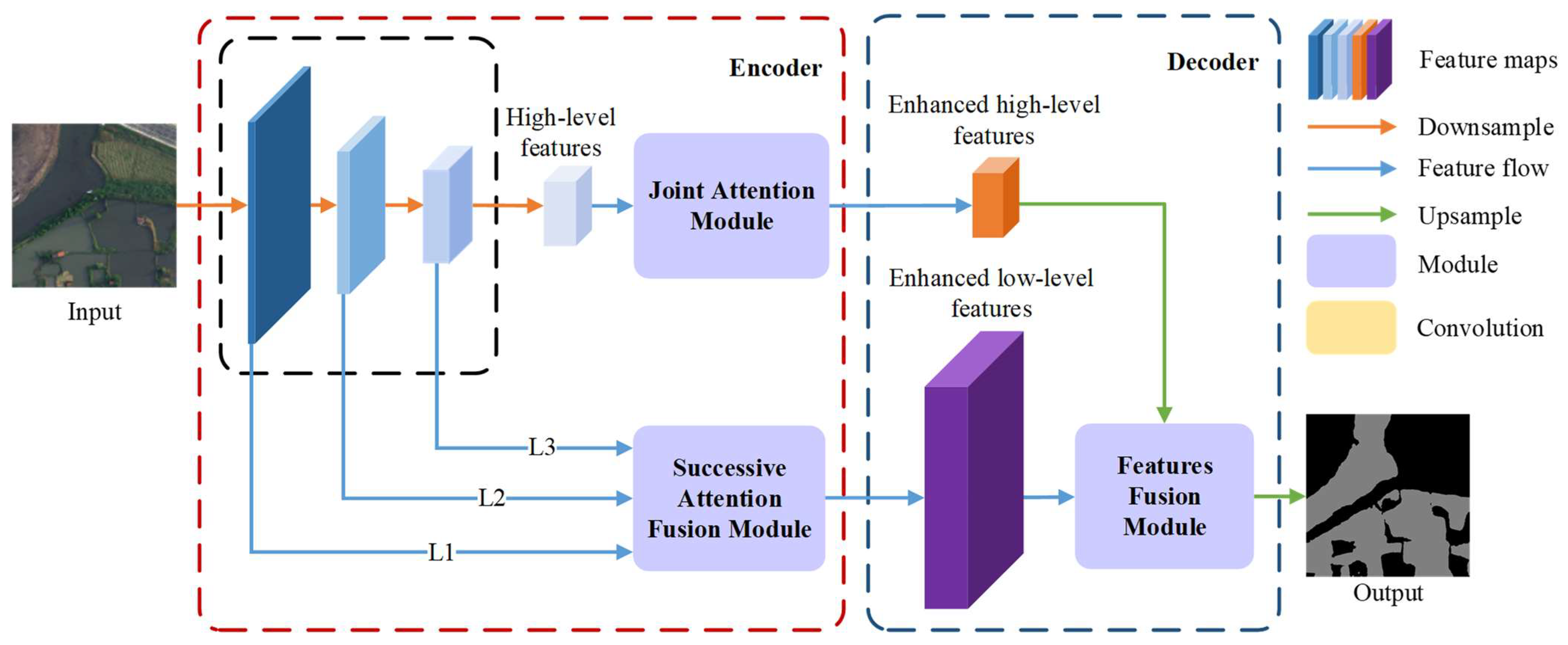
  • Based on the encoder–decoder architecture, MSAFNet gradually extracts semantic information and spatial details at multiple scales. In particular, a feature fusion module (FFM) was designed to aggregate and align multi-level features, alleviating the uncertainty in delineating boundaries and making the proposed model more accurate in extracting water bodies.
  • A successive attention fusion module (SAFM) is proposed to enhance multi-level features in local regions of the feature map, refining multiscale features parallelly and extracting correlations between hierarchical channels. As a result, the multiscale features are extracted and aggregated adaptively, providing a sufficient contextual representation of various water bodies.
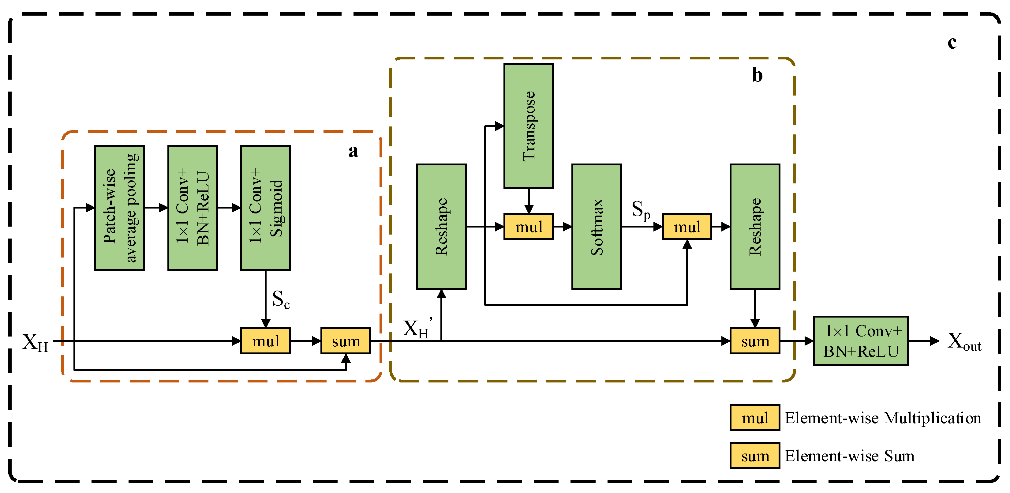
  • To enhance the distinguishability of semantic representations, a joint attention module (JAM) was designed. It utilizes position self-attention block (PSAB) to make similar features related to each other regardless of distance to aggregate the features of each position selectively, strengthening the proposed network in resisting noise interference.

2. Related Works

2.1. Encoder–Decoder Architecture

Encoder–decoder-structured CNNs are commonly used in computer vision tasks, including image restoration [32] and saliency detection [33]. These networks consist of two stages: (1) an encoder stage, which reduces noise and captures higher semantic information at the trade-off of reduced image resolution, and (2) a decoder stage, which recovers spatial information through an upsampling strategy. Finally, image reconstruction is used to output predicted results. Since FCN was proposed, the architecture has been widely used in semantic segmentation. To improve the models’ semantic segmentation performance, some studies have focused on facilitating contextual information fusion or expanding the receptive field. Examples are PSPNet [16], DeepLabV3+ [17], and SegNet [34]. Additionally, some studies introduce attention mechanisms at the encoder stage to capture local contextual information. For instance, LANet integrated the PAM and AEM modules based on the encoder–decoder structure to enhance feature expression ability [35]. Moreover, some models [36,37,38] accurately capture multiscale features by increasing the network depth or introducing dense skip connections, which are effective but not efficient.
The encoder–decoder structure plays a pivotal role in mining and aggregating multiscale visual features. However, existing encoder–decoder-structured models suffer from two problems, namely a limited ability to capture multiscale semantic information and spatial details during the encoder part, and insufficient fusion of multi-level features in the decoder. Therefore, MSAFNet adopts the architecture, on which we have improved.

2.2. Multi-Level Feature Aggregation

It is well known that contextual information is crucial for the semantic segmentation of RSIs [39,40,41]. Traditional feature fusion methods can be divided into spatial fusion and semantic fusion [42]. Semantic fusion is represented by skip connections, where features are fused sequentially between different levels and losses are better propagated, allowing spatial details to be preserved. Spatial fusion, such as feature pyramid networks, is used to obtain more homogeneous resolution and normalized semantic information through top–down and lateral connections. For example, in UNet++, a combination of skip connections and short connections is used to facilitate semantic fusion between feature maps at different levels to bridge the feature gap at multiple levels [43]. Liu et al., in 2021, proposed the U²-Net, which mixes different residual U-shaped blocks (RSUs) that have different-sized receptive fields to capture more contextual information. This model uses multiple U-shaped structures to make the model better adapted to semantic segmentation, improving the robustness of the model [44].
However, traditional feature fusion methods cannot effectively aggregate features at multiple levels, resulting in segmentation models lacking the ability to efficiently identify water bodies at different scales. To address this problem, some studies have introduced attention-based feature fusion methods in the models. For example, the SFAM utilizes the local relationships of advanced features as attention scores to promote the semantic fusion of multi-level features effectively [45]. Peng et al., achieved the cross-fusion of multiscale features through CARB and CF blocks to improve the capture capability of the cross fusion network (CFNet) for small-scale objects [46].
These multi-level feature fusion methods aim to aggregate multiscale features and find consistency in contextual information. However, the methods are not strong enough in capturing informative features. To effectively capture spatial details and semantic features of multiscale water bodies, the idea of the successive attention fusion method is embedded into the proposed model, so that the model’s performance can be improved.

2.3. Attention Mechanism

The design of the attention mechanism is inspired by the human visual system. In application to the semantic segmentation of natural images, various attention mechanisms are introduced into models, which have achieved great performance in mining visual features [47,48]. In SENet, SE block was proposed to enhance the correlation of inter-channel features using a global averaging pooling operation in the channel dimension [49]. A non-local block is constructed in non-local neural networks, where all pixels are weighted according to the correlation between each pixel [50]. The CBAM [51] uses the channel and spatial attention module sequentially, and two operations, maximum pooling and average pooling, are used in these modules to highlight and preserve contextual information. In DANet, the global dependencies of space and channel are used in a parallel manner so that adequate semantic representation is captured by the model [52].
Over the past years, many different attention modules have been designed for the semantic segmentation of RSIs [53,54]. DEANet extracts multiscale information by introducing pyramid sampling into the channel dimension [55]. To obtain better representation, a novel attention-based framework named HMANet was proposed to capture long-range dependencies [56]. MSNANet proposed the MSNA and OASPP modules, which effectively merge multiscale water body features and refine the representation by leveraging contextual information to improve the models’ water body extraction accuracy [57]. HA-Unet enhances the ability to capture shallow feature details and enhance global contextual information through the joint use of local attention and self-attention, achieving effective extraction of complex urban water bodies [58].
In summary, MSAFNet combines the attention mechanism with multi-level feature aggregation. The former is able to effectively capture multiscale water body features while improving the distinguishability for semantic representation. The latter helps to adaptively aggregate multiscale water bodies and refine the multiscale and multi-shape feature representation of water bodies.

3. The Proposed Method

This section introduces MSAFNet, which aims to achieve high accuracy in water body extraction. First, a general overview and the core idea of the network are given. This is followed by a detailed description of the structure and functionality of all the modules.

3.1. Overview of the MSAFNet

Mining and aggerating multiscale semantic information is an effective strategy to improve extraction accuracy. The shape and size of water bodies in RSIs are complex and variable (such as canals, ponds, rivers, and lakes), and so the extraction of multiscale water bodies by some models is highly likely to be blurred. Therefore, MSAFNet uses modules, named SAFM, JAM, and FFM, to improve the ability to recognize multiscale and multi-shape water bodies from RSIs.
The architecture of MSAFNet is shown in Figure 1, and it consists of two main parts. First, we use the pre-trained ResNet50 to extract multi-level features. Then, the SAFM parallelly refines the multi-level feature maps by patch-based local attention method, so that size-varied water-related objects can be better extracted adaptively. Simultaneously, the JAM enhances the advanced features to suppress noise interference. In the decoder stage, the multi-level features are fed into the FFM to aggregate the spatial details and abstract semantic information to alleviate the problem of blurred water body boundaries. Finally, convolution and upsampling are used to output the predicted water body extraction results.

3.2. Successive Attention Fusion Module

Unlike natural images, the detailed information of segmented objects on remotely sensed images is more difficult to capture. Furthermore, as the model deepens, fine-grained spatial details at different scales, especially at shallow layers, are damaged. Thus, the convolution and pooling operations alone are insufficient to extract multiscale water bodies.
To alleviate the problem above-mentioned, we design the SAFM inspired by the design of PAM [35]. The SAFM uses Single-level Attention Block (SAB) to adaptively select informative features from the feature maps of different levels to identify multiscale water bodies in RSIs. Let us first consider a single feature map X R C × H × W , where C , H and W denote the channel, height and width of the feature map, and then the feature map is divided into several non-overlapping square regions. The operation that generates the local weight vector z p c of the region p at channel c is called Patch-Squeeze operation and is expressed as
z p c = 1 h p × w p i = 1 h p j = 1 w p x c ( i , j )
where h p and w p represent the height and width of the pooling window, respectively, and x c ( i , j ) represents the value of a pixel on channel c . After the above operation, a local weight information z is generated, indicating whether the region is worthy of attention or not. Then, the Patch-Excitation operation is performed to compute the attention score. The score map S R C × H × W can be obtained by the following formula:
S = F U { σ [ W 2 δ ( W 1 z ) ] }
where W 1 and W 2 denote the 1 × 1 dimension-reduction and dimension-increasing convolution, respectively, δ denotes normalization and ReLU functions [59], σ denotes the Sigmoid function, and F U denotes the upsampling operation. Lastly, a residual design is added to get the stability of the gradient backpropagation. This step is implemented as follows:
X L k = X ( S X )
where and refer to the elementwise sum and multiplication, respectively, and X L k represents the k th level’s feature map.
Figure 2 shows the pipeline of the SAFM, which extracted multiscale local features by SABs. X c o n c a t can be symbolized by the following formula:
X c o n c a t = c o n c a t [ X L 1 , F U ( X L 2 ) , F U ( X L 3 ) ]
where F U and c o n c a t denote the upsampling and concatenation operations, respectively. Then, the SAFM applies multi-level fusion block (MFB) to fuse multi-level features by the global layer-level attention method. The enhanced X o u t L R C l × H l × W l values are calculated as
X o u t L = σ [ W 2 δ ( W 1 X c o n c a t ) ]
where W 1 and W 2 represents the 1 × 1 dimension-reduction and dimension-increasing convolutions, respectively; δ denotes normalization and ReLU functions, and σ denotes the Sigmoid function.
By adopting a strategy of aggregating multi-level features after enhancing single-level features, the SAFM is able to retain local feature information and reduce noise. At the same time, a channel attention mechanism is used to capture the spectral information of multiscale water bodies, thereby effectively aggregating multi-level feature representations. Notably, the SAFM controls the size of the pooling window proportionally in each SAB, achieving the effect of successive enhancement to the same region of the multi-level features.

3.3. Joint Attention Module

To further mine and select the informative features, the JAM was designed, which embeds contextual dependencies into representations through joint modeling. In Figure 3a, X H R C h × H h × W h is inputted to the patch-based local attention block (PLAB), and the weight vector is generated using an average pooling operation with a pooling window of 2 × 2 and a move step of 1. Then, the 1 × 1 convolution with BN and ReLU operations is used for dimension reduction; the 1 × 1 convolution with the Sigmoid operation is used for dimension recovery. Finally, S c is residual connected with X H to obtain X H . Figure 3b shows the PSAB, which performs spatial self-attention operation on the features to capture the spatial similarity between two pixels, so that the proposed model’s ability in resisting noise interference can be strengthened.
Overall, PLAB focuses on the local contextual information of the high-level feature map to enhance the channel relevance of local features. Then, PSAB is used to extract the information correlation between pixels in the spatial dimension. As shown in Figure 3c, after using PLAB and PSAB, the advanced feature map achieves reduced dimensionality, to which the 1 × 1 convolution is applied with BN and ReLU functions to output X o u t H .

3.4. Features Fusion Module

In order to fuse multiscale contextual information, CNNs have inevitably extracted multi-level features by deepening the network depth; however, this blind approach ignores the differences in the feature maps at different levels, which leads to frustrated stability and performance of the models. Therefore, there is a need to facilitate multi-level feature aggregation, which simultaneously captures spatial details and semantic information of multiscale water bodies, to improve extraction performance. To make the most of advanced features and low-level spatial details, the FFM fuses and aligns them to alleviate the uncertainty in delineating boundaries. As shown in Figure 4, X H R C h × H h × W h after the JAM is inputted into the FFM and X L R C l × H l × W l after the SAFM is inputted into the FFM. After the features of different levels are concatenated together, the 3 × 3 convolution with BN and ReLU functions is applied to aggregate multi-level feature information and reduce dimensionality. Then, the weight vectors on the channel dimension are obtained using global pooling operations, and the FFM performs one downscaling and one upscaling operation on the weight vector to facilitate global feature information fusion. Finally, the 1 × 1 convolution is used to output the predicted results. In general, the FFM improves feature distinguishability and accelerates network convergence, which aids in performance.
With the combined effect of these modules, more accurate semantic information from different scales is extracted.

4. Experiments

In this section, the datasets, experimental details, and evaluation metrics are first presented, followed by the experimental results and the ablation study.

4.1. Datasets

To evaluate the effectiveness of MSAFNet, experiments were conducted on two datasets, namely the Qinghai-Tibet Plateau Lake dataset (QTPL) [21] and the Land-cOVEr Domain Adaptive semantic segmentation dataset (LoveDA) [60].

4.1.1. The QTPL Dataset

The public QTPL dataset is captured on the Tibetan Plateau, which consists of 6774 remote sensing images. The dataset is composed of red–green–blue (RGB) three-channel images with a size of 256 × 256 pixels, among which only lakes were labeled using labelme. Therefore, RSIs contain only two label types: water body and background. In our experiments, we selected 6069 images to build the testing set, and the rest were used to construct the training set.
The lakes on the Tibetan Plateau are characterized by indistinguishable spectral features. The white lakes have features such as snow, while the black lakes have features including mountains and cloud shadows. Therefore, this dataset can effectively test the model’s ability to extract water bodies.

4.1.2. The LoveDA Dataset

The dataset is an urban–rural domain adaptive ground cover dataset that can be utilized for water body extraction. This dataset is constructed from images with a non-overlapping cover size of 1024 × 1024 and a spatial resolution of 0.3 m. The images in the dataset cover the location information of objects in three regions: Nanjing, Changzhou, and Wuhan. All images were geometrically corrected and preprocessed, and each of them contains three channels of red–green–blue.
To apply the LoveDA dataset to the water body extraction, urban and rural images were randomly selected from which multiscale and multi-shape water bodies, such as reservoirs and rivers, were positively annotated. Figure 5 shows the rural and urban images and their reference maps. Due to computational resource constraints, the input data for the training phase were all cropped without overlap using a 256 × 256 window, resulting in 63,050 training images and 15,750 testing images.

4.2. Experimental Details

The experimental device operating system was Ubuntu 18.04, and the GPU was NVIDIA A40. Pytorch was used for model training, and the version of Python was 3.8.13. The max epoch number and batch size were set to 200 and 16, respectively. In each iteration, the RSIs in the training set were disordered to enhance the generalization capability of the models. To train our network, we used ReduceLROnPlateau to reduce the learning rate gradually. Root Mean Square prop [61] (RMSProp) with a momentum of 0.9 was used as the optimizer to update the model parameters, and the initial learning rate was set to 2 × 10⁻⁵. All models use the cross-entropy (CE) loss as the loss function, and the formula is expressed as follows:
L C E = i = 1 n y i log ( y ^ i )
where y i and y ^ i are the ground truth and the predicted results, respectively.

4.3. Evaluation Metrics

To effectively evaluate the performance of all models, the following metrics are used: overall accuracy (OA), F1, Kappa, Mean Intersection over Union (MIoU), and Frequency Weight Intersection over Union (FWIoU). Usually, precision and recall are contradictory to each other, so F1 is applied to reconcile them. Meanwhile, MIoU is used to obtain a comprehensive evaluation of the extraction results. On the other hand, the model prefers to predict pixels as background pixels, because of the unbalanced distribution of pixels between backgrounds and water bodies in the datasets. To address this problem, Kappa and FWIoU are used. The definitions of T P , F P , T N , and F N are listed in Table 1, and the related equations are as follows:
p r e c i s i o n = T P T P + F P
r e c a l l = T P T P + F N
F 1 = 2 × p r e c i s i o n × r e c a l l p r e c i s i o n + r e c a l l
p 0 = OA = T P + T N T P + T N + F P + F N
p e = ( T P + T N ) × ( T P + F P ) + ( F P + F N ) × ( T N + F N ) N 2
K a p p a = p 0 p e 1 p e
M I o U = 1 k + 1 i = 0 k T P F N + T P + F P
F W I o U = i = 0 k [ ( T P + F N T P + F P + T N + F N × T P T P + F P + F N ) ]

4.4. Experimental Results

To verify the performance of MSAFNet, the model was experimentally compared to the eleven different models mentioned in this research: UNet, PSPNet, DeepLabV3+, UNet++, U2-Net, Attention-UNet, FCN + CBAM, FCN + DA, FCN + SE, MSNANet, and LANet. A related study was conducted on the QTPL and LoveDA datasets, where the numbers in bold in the tables indicate the best results.

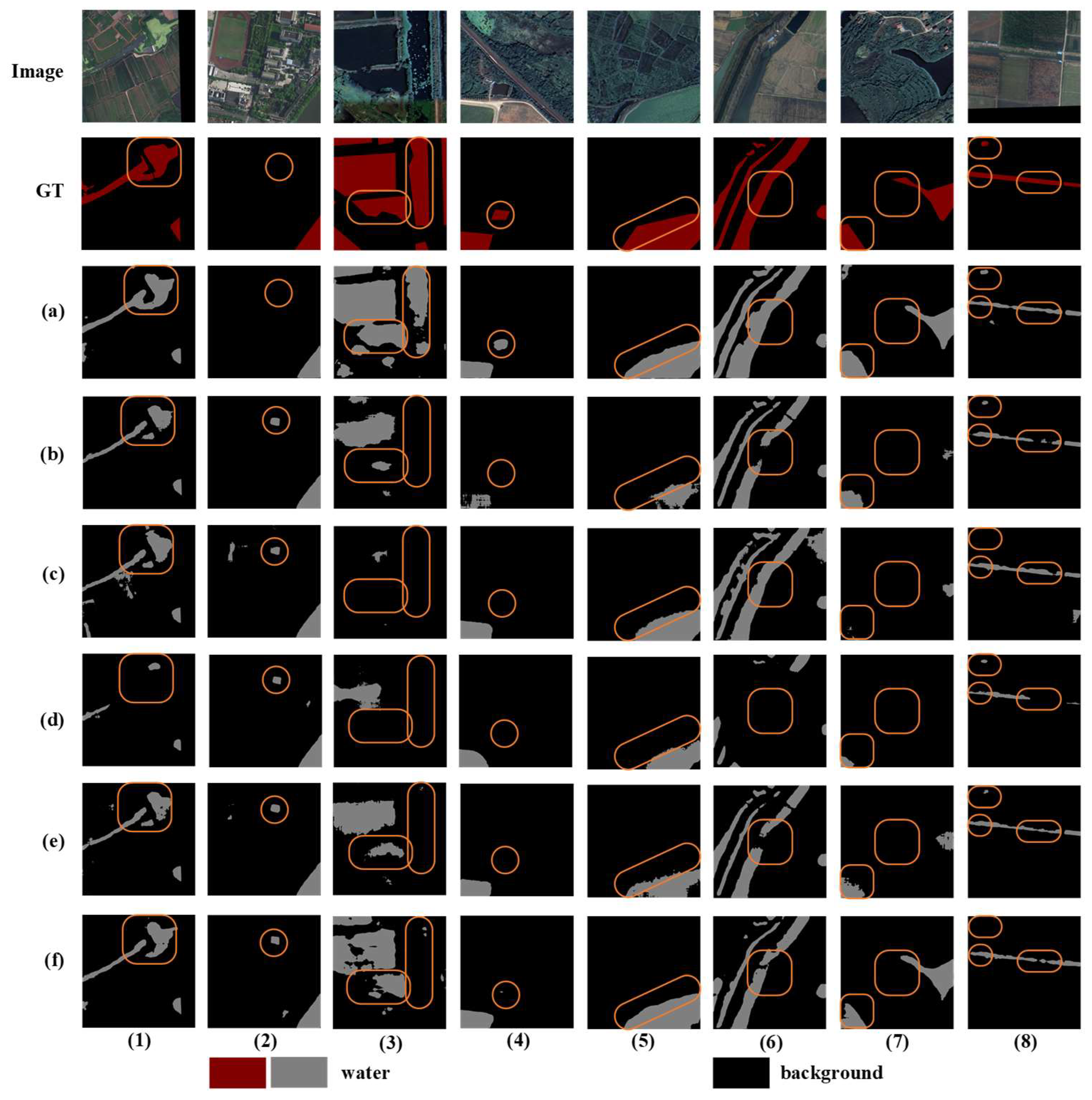
4.4.1. Results on the QTPL Dataset

As summarized in Table 2, MSAFNet has the highest Kappa, MIoU, FWIoU, F1, and OA (0.9786, 97.88%, 97.96%, 99.14%, and 98.97%, respectively). UNet++ and U2-Net with multiscale feature fusion modules perform well, too. Compared with U²Net, which is second only to MSAFNet in model performance, the evaluation metrics of MSAFNet improve by 0.0019, 0.18%, 0.18%, 0.08%, and 0.09% for Kappa, MIoU, FWIoU, F1, and OA, respectively. LANet is less capable of extracting water boundaries than UNet++, but its calculation complexity is lower. On the other hand, the models containing the lightweight attention modules (CBAM, DA, and SE) also achieve a good performance. However, AttentionUNet, which uses the attention gates, does not perform satisfactorily for water body extraction on both datasets as it ignores the inherent characteristics of RSIs. Similarly, although the classic models (UNet, PSPNet, and DeepLabV3+) are suitable for semantic segmentation in natural scenes, their results for water body extraction are not satisfactory.
Figure 6 shows visualizations of the MSAFNet and other models on the QTPL dataset. The water bodies in the QTPL dataset are characterized by multiscale and multi-shape. In addition, noise such as salt bands, mountain shadows, snow, and clouds can make it challenging to segment water bodies. AttentionUNet, UNet++, and DeepLabV3+ can only partially identify small water bodies and water body boundaries, while all lack resistance to noises. U2-Net uses residual U-blocks and two nested U-shapes to compensate for the variability of feature maps, and its good performance of multiscale feature fusion gives the model good interference resistance (d6–d8). However, U2-Net cannot analyze the water body boundary well (d1,d2). LANet uses semantic information to guide multiscale spatial details [30], which is effective in identifying large-scale water bodies (f7) but also leads to blurring water body boundary segmentation (f1,f5). Finally, MSAFNet can make water body boundaries well-mapped and resistant to noise such as glaciers and clouds. So, compared with other models, the inferred results of MSAFNet are closest to the labels of water bodies.

4.4.2. Results on the LoveDA Dataset

The quantitative comparisons on the LoveDA dataset are summarized in Table 3. The dataset contains both urban and rural scene styles, resulting in very large differences in the scale of water bodies in complex scenes. In addition, the representation of water bodies in remotely sensed imagery is disturbed by a wide range of noise. Among these twelve models, MSAFNet performs the best, achieving the best results in all evaluation metrics (Kappa, MIoU, FWIoU, F1, and OA of 0.7844, 81.58%, 92.17%, 97.69%, and 95.87%, respectively). On the one hand, traditional convolutional models such as PSPNet, UNet, and DeepLabV3+ are unable to extract water body information accurately and efficiently, even if the receptive field is expanded by skip connections and atrous convolution. However, multi-level feature fusion models (U2-Net and UNet++), which improve on the traditional semantic segmentation structure, can aggregate multiscale feature information to achieve better performance. Overall, the model using cross-layer fusion outperformed the model with in-module fusion in this dataset. On the other hand, LANet focuses on the water body representation at different scales through local attention operations, which improves the extraction accuracy to a certain extent but also ignores the global contextual information. Additionally, the models using lightweight attention mechanisms (SE, CBAM, DA, etc.) enhanced the extracted features and all achieved great results.
Figure 7 shows the visualizations on the LoveDA dataset. On the one hand, MSAFNet can extract small water bodies (a4,a8), linear continuous water bodies (a6–a8), and their boundaries (a1,a3,a5), because of its ability to preserve features of size-varied water bodies. MSAFNet can also resist noise interference such as building shadows (a2). So, MSAFNet outperforms other models and the visualizations are better than other models.
The parametric quantities (Params) and computational complexity (FLOPS) of these models are listed in Table 4. In general, the proposed model uses less computational cost and is more effective than the contextual information aggregation-based models (PSPNet, DeepLabV3+, U2Net, etc.). The MSAFNet does not increase the computational effort significantly compared with attention-based approaches (SE, CBAM, DA, etc.), but achieves better extraction performance.

4.5. Ablation Study

In the ablation experiments, MSAFNet was trained and evaluated on the QTPL and LoveDA datasets. Firstly, the SAFM was tested by inputting different levels of feature maps to verify that each feature map can be used reasonably well by the module. As shown in Table 5, for the QTPL dataset, MIoU, F1, and OA decreased by 0.05%, 0.02%, and 0.03%, respectively, when the L1 feature map was not used. The decreasing trend of the evaluation metrics was even more pronounced when the L1 and L2 feature maps were both not used, with MIoU, F1, and OA decreasing by 0.17%, 0.08%, and 0.09%, respectively. On the other hand, this gap was more pronounced on the LoveDA dataset, where the evaluation metrics MIoU, F1, and OA decreased by 0.76%, 0.04%, and 0.10%, respectively, when the L1 feature map was not used, and by 1.07%, 0.05%, and 0.12%, respectively, when the L1 and L2 feature maps were both not used. This implies that, by fusing multi-level features, the SAFM can effectively improve model performance with an acceptable increase in parameters and computational burden.
First, we used FCN(ResNet-50) as the backbone. As shown in Table 6, when only the JAM (added at the end of the FCN encoder) is used, the boosts for each evaluation metric (MIoU, F1, OA) are 0.09%, 0.04%, and 0.04%, respectively; the evaluation metrics improve by 0.47%, 0.21%, and 0.23%, respectively, when only the SAFM (added at the decoder stage to capture multi-level features) is used. Then, when both the JAM and the SAFM are used, high-level and lower-level features are fused by concatenation. This fusion is not sufficient, leading the evaluation metrics to not improve much or even decrease. Finally, the proposed MSAFNet uses the JAM, SAFM, and FFM, resulting in improved model performance and significant improvement in evaluation metrics of 0.67%, 0.29%, and 0.33%, respectively.
Table 7 shows the results on the LoveDA dataset, and they also indicate the three modules’ great performance. The difference is that the RSIs in the LoveDA dataset have more complex scene information and more noisy information such as shrubs in the countryside and the shadows of tall buildings in urban areas. Therefore, the model using only the JAM achieved significant segmentation results than the baseline network with the SAFM. Furthermore, the FFM is used to compensate for differences in global contextual information for multi-layered features, improving the accurate mapping of water body boundaries.
As shown in Figure 8, the visualizations suggest that the JAM can extract large lakes (e) and enhance the model’s resistance to noise (noise such as glaciers) interference (c), while the SAFM is useful to map small-scale objects such as small lakes (a and c). On the other hand, when the FFM is removed, the spatial and geometric information between different-level features cannot be effectively fused. Overall, the results show that the SAFM and JAM can help the model refine the multiscale feature representation of water bodies, while the FFM can better map the fine-grained features of water body edges and improve the extraction performance of the model.

5. Conclusions

We developed a water body extraction model called MSAFNet for capturing the semantic information of multiscale and multi-shape water bodies. It consists of three modules, i.e., the SAFM, JAM, and FFM. In particular, the SAFM, which organically couples attention mechanism with multi-level feature aggregation, is proposed to excavate key information from shallow layers and aggregate them adaptively, so as to extract fine-size-varied water bodies effectively and efficiently. Through the JAM, MSAFNet allows similar features correlated to each other to selectively aggregate the feature of each position, so the informative features are further mined and the model’s resistance to noise can be enhanced. Furthermore, the FFM fuses the multiscale semantic information and space details, which alleviates the inaccurate segmentation of water bodies’ edges.
Extensive experiments have been conducted on the QTPL and the LoveDA datasets. The SAFM and JAM can accurately capture fine-grained multiscale features, allowing rich spatial information and semantic features to be aggregated by the FFM, enhancing the model’s water extraction performance. The effectiveness of the modules is indicated by conducting ablation experiments on both datasets as well. Therefore, multiscale water bodies and boundaries are well-delineated by MSAFNet. According to numerical evaluations and visual inspections, MSAFNet exhibits competitive performance. However, in the future, we will further improve the models to adapt to different scenarios with fewer available data. In addition, we plan to improve models for automated water body interpretation from hyperspectral images to address the accuracy of water body extraction for different water qualities.

Author Contributions

Conceptualization, X.L. (Xin Lyu) and W.J.; methodology, W.J.; software, W.J.; validation, X.L. (Xin Lyu) and W.J.; formal analysis, X.L. (Xin Li); investigation, W.J. and X.L. (Xin Li); resources, X.L. (Xin Lyu), Z.X. and X.L. (Xin Li); data curation, W.J. and X.W.; writing—original draft preparation, W.J.; writing—review and editing, X.L. (Xin Lyu) and X.L. (Xin Li); visualization, X.L. (Xin Lyu) and W.J.; supervision, X.L. (Xin Lyu); project administration, Y.F. and X.L. (Xin Lyu); funding acquisition X.L. (Xin Lyu). All authors have read and agreed to the published version of the manuscript.

Funding

This research was funded by the Excellent Post-doctoral Program of Jiangsu Province (grant no. 2022ZB166), the Fundamental Research Funds for the Central Universities (grant no. B230201007), the Project of Water Science and Technology of Jiangsu Province (grant no. 2021080, 2021063), the National Natural Science Foundation of China (grant no. 42104033, 42101343, and 82004498, the Joint Fund of Ministry of Education for Equipment Pre-research (grant no. 8091B022123), the Research Fund from Science and Technology on Underwater Vehicle Technology Laboratory (grant no. 2021JCJQ-SYSJJ-LB06905), and the Qinglan Project of Jiangsu Province.

Data Availability Statement

The datasets in our study are public. The Qinghai-Tibet Plateau Lake dataset can be found at http://www.ncdc.ac.cn/portal/metadata/b4d9fb27-ec93-433d-893a-2689379a3fc0 (accessed on 16 March 2023). The Land-cOVEr Domain Adaptive semantic segmentation dataset can be found at https://drive.google.com/drive/folders/1ibYV0qwn4yuuh068Rnc-w4tPi0U0c-ti (accessed on 16 March 2023).

Conflicts of Interest

The authors declare no conflict of interest.

References

  1. Weng, Q. Remote Sensing of Impervious Surfaces in the Urban Areas: Requirements, Methods, and Trends. Remote Sens. Environ. 2012, 117, 34–49. [Google Scholar] [CrossRef]
  2. Hu, T.; Yang, J.; Li, X.; Gong, P. Mapping Urban Land Use by Using Landsat Images and Open Social Data. Remote Sens. 2016, 8, 151. [Google Scholar] [CrossRef]
  3. Kuhn, C.; de Matos Valerio, A.; Ward, N.; Loken, L.; Sawakuchi, H.O.; Kampel, M.; Richey, J.; Stadler, P.; Crawford, J.; Striegl, R.; et al. Performance of Landsat-8 and Sentinel-2 Surface Reflectance Products for River Remote Sensing Retrievals of Chlorophyll-a and Turbidity. Remote Sens. Environ. 2019, 224, 104–118. [Google Scholar] [CrossRef] [Green Version]
  4. Zhang, W.; Li, X.; Yu, J.; Kumar, M.; Mao, Y. Remote Sensing Image Mosaic Technology Based on SURF Algorithm in Agriculture. J. Image Video Proc. 2018, 2018, 85. [Google Scholar] [CrossRef]
  5. Yang, G.; Li, B.; Ji, S.; Gao, F.; Xu, Q. Ship Detection From Optical Satellite Images Based on Sea Surface Analysis. IEEE Geosci. Remote Sens. Lett. 2014, 11, 641–645. [Google Scholar] [CrossRef]
  6. Xu, N.; Gong, P. Significant Coastline Changes in China during 1991–2015 Tracked by Landsat Data. Sci. Bull. 2018, 63, 883–886. [Google Scholar] [CrossRef] [Green Version]
  7. Ma, Y.; Xu, N.; Sun, J.; Wang, X.H.; Yang, F.; Li, S. Estimating Water Levels and Volumes of Lakes Dated Back to the 1980s Using Landsat Imagery and Photon-Counting Lidar Datasets. Remote Sens. Environ. 2019, 232, 111287. [Google Scholar] [CrossRef]
  8. Xu, N.; Ma, Y.; Zhang, W.; Wang, X.H. Surface-Water-Level Changes During 2003–2019 in Australia Revealed by ICESat/ICESat-2 Altimetry and Landsat Imagery. IEEE Geosci. Remote Sens. Lett. 2021, 18, 1129–1133. [Google Scholar] [CrossRef]
  9. Rahnemoonfar, M.; Chowdhury, T.; Sarkar, A.; Varshney, D.; Yari, M.; Murphy, R.R. FloodNet: A High Resolution Aerial Imagery Dataset for Post Flood Scene Understanding. IEEE Access 2021, 9, 89644–89654. [Google Scholar] [CrossRef]
  10. Chen, Z.; Lu, Z.; Gao, H.; Zhang, Y.; Zhao, J.; Hong, D.; Zhang, B. Global to Local: A Hierarchical Detection Algorithm for Hyperspectral Image Target Detection. IEEE Trans. Geosci. Remote Sens. 2022, 60, 1–15. [Google Scholar] [CrossRef]
  11. Feyisa, G.L.; Meilby, H.; Fensholt, R.; Proud, S.R. Automated Water Extraction Index: A New Technique for Surface Water Mapping Using Landsat Imagery. Remote Sens. Environ. 2014, 140, 23–35. [Google Scholar] [CrossRef]
  12. Paul, A.; Tripathi, D.; Dutta, D. Application and Comparison of Advanced Supervised Classifiers in Extraction of Water Bodies from Remote Sensing Images. Sustain. Water Resour. Manag. 2018, 4, 905–919. [Google Scholar] [CrossRef]
  13. Zhang, L.; Zhang, L.; Du, B. Deep Learning for Remote Sensing Data: A Technical Tutorial on the State of the Art. IEEE Geosci. Remote Sens. Mag. 2016, 4, 22–40. [Google Scholar] [CrossRef]
  14. Shelhamer, E.; Long, J.; Darrell, T. Fully Convolutional Networks for Semantic Segmentation. IEEE Trans. Pattern Anal. Mach. Intell. 2017, 39, 640–651. [Google Scholar] [CrossRef] [PubMed]
  15. Ronneberger, O.; Fischer, P.; Brox, T. U-net: Convolutional networks for biomedical image segmentation. In Proceedings of the International Conference on Medical Image Computing and Computer-Assisted Intervention (MICCAI), Munich, Germany, 5–9 October 2015; pp. 234–241. [Google Scholar]
  16. Zhao, H.; Shi, J.; Qi, X.; Wang, X.; Jia, J. Pyramid Scene Parsing Network. In Proceedings of the IEEE Conference on Computer Vision and Pattern Recognition (CVPR), Honolulu, HI, USA, 21–26 July 2017; pp. 6230–6239. [Google Scholar]
  17. Chen, L.; Zhu, Y.; Papandreou, G.; Schroff, F.; Adam, H. Encoder-decoder with atrous separable convolution for semantic image segmentation. In Proceedings of the European Conference on Computer Vision (ECCV), Munich, Germany, 8–14 September 2018; pp. 801–818. [Google Scholar]
  18. Chen, Y.; Fan, R.; Yang, X.; Wang, J.; Latif, A. Extraction of Urban Water Bodies from High-Resolution Remote-Sensing Imagery Using Deep Learning. Water 2018, 10, 585. [Google Scholar] [CrossRef] [Green Version]
  19. Isikdogan, F.; Bovik, A.C.; Passalacqua, P. Surface Water Mapping by Deep Learning. IEEE J. Sel. Top. Appl. Earth Obs. Remote Sens. 2017, 10, 4909–4918. [Google Scholar] [CrossRef]
  20. Weng, L.; Xu, Y.; Xia, M.; Zhang, Y.; Liu, J.; Xu, Y. Water Areas Segmentation from Remote Sensing Images Using a Separable Residual SegNet Network. ISPRS Int. J. Geo-Inf. 2020, 9, 256. [Google Scholar] [CrossRef]
  21. Wang, Z.; Gao, X.; Zhang, Y.; Zhao, G. MSLWENet: A Novel Deep Learning Network for Lake Water Body Extraction of Google Remote Sensing Images. Remote Sens. 2020, 12, 4140. [Google Scholar] [CrossRef]
  22. Xia, M.; Cui, Y.; Zhang, Y.; Xu, Y.; Liu, J.; Xu, Y. DAU-Net: A Novel Water Areas Segmentation Structure for Remote Sensing Image. Int. J. Remote Sens. 2021, 42, 2594–2621. [Google Scholar] [CrossRef]
  23. Li, H.; Qiu, K.; Chen, L.; Mei, X.; Hong, L.; Tao, C. SCAttNet: Semantic Segmentation Network with Spatial and Channel Attention Mechanism for High-Resolution Remote Sensing Images. IEEE Geosci. Remote Sens. Lett. 2021, 18, 905–909. [Google Scholar] [CrossRef]
  24. Miao, Z.; Fu, K.; Sun, H.; Sun, X.; Yan, M. Automatic Water-Body Segmentation from High-Resolution Satellite Images via Deep Networks. IEEE Geosci. Remote Sens. Lett. 2018, 15, 602–606. [Google Scholar] [CrossRef]
  25. Xu, Z.; Zhang, W.; Zhang, T.; Li, J. HRCNet: High-Resolution Context Extraction Network for Semantic Segmentation of Remote Sensing Images. Remote Sens. 2021, 13, 71. [Google Scholar] [CrossRef]
  26. Sun, L.; Cheng, S.; Zheng, Y.; Wu, Z.; Zhang, J. SPANet: Successive Pooling Attention Network for Semantic Segmentation of Remote Sensing Images. IEEE J. Sel. Top. Appl. Earth Obs. Remote Sens. 2022, 15, 4045–4057. [Google Scholar] [CrossRef]
  27. Li, A.; Jiao, L.; Zhu, H.; Li, L.; Liu, F. Multitask Semantic Boundary Awareness Network for Remote Sensing Image Segmentation. IEEE Trans. Geosci. Remote Sens. 2022, 60, 1–14. [Google Scholar] [CrossRef]
  28. Deng, G.; Wu, Z.; Wang, C.; Xu, M.; Zhong, Y. CCANet: Class-Constraint Coarse-to-Fine Attentional Deep Network for Subdecimeter Aerial Image Semantic Segmentation. IEEE Trans. Geosci. Remote Sens. 2022, 60, 1–20. [Google Scholar] [CrossRef]
  29. Li, X.; Xu, F.; Lyu, X.; Gao, H.; Tong, Y.; Cai, S.; Li, S.; Liu, D. Dual Attention Deep Fusion Semantic Segmentation Networks of Large-Scale Satellite Remote-Sensing Images. Int. J. Remote Sens. 2021, 42, 3583–3610. [Google Scholar] [CrossRef]
  30. Liu, R.; Tao, F.; Liu, X.; Na, J.; Leng, H.; Wu, J.; Zhou, T. RAANet: A Residual ASPP with Attention Framework for Semantic Segmentation of High-Resolution Remote Sensing Images. Remote Sens. 2022, 14, 3109. [Google Scholar] [CrossRef]
  31. Ding, Y.; Zhang, Z.; Zhao, X.; Hong, D.; Cai, W.; Yang, N.; Wang, B. Multi-Scale Receptive Fields: Graph Attention Neural Network for Hyperspectral Image Classification. Expert Syst. Appl. 2023, 223, 119858. [Google Scholar] [CrossRef]
  32. Zamir, S.W.; Arora, A.; Khan, S.; Hayat, M.; Khan, F.S.; Yang, M.-H.; Shao, L. Multi-Stage Progressive Image Restoration. In Proceedings of the 2021 IEEE/CVF Conference on Computer Vision and Pattern Recognition (CVPR), Online, 19–25 June 2021; IEEE: Nashville, TN, USA, 2021; pp. 14816–14826. [Google Scholar]
  33. Zhao, Z.; Xia, C.; Xie, C.; Li, J. Complementary Trilateral Decoder for Fast and Accurate Salient Object Detection. In Proceedings of the 29th ACM International Conference on Multimedia, MM 2021, Online, 20–24 October 2021; Association for Computing Machinery, Inc.: Beijing, China, 2021; pp. 4967–4975. [Google Scholar]
  34. Badrinarayanan, V.; Kendall, A.; Cipolla, R. SegNet: A Deep Convolutional Encoder-Decoder Architecture for Image Segmentation. IEEE Trans. Pattern Anal. Mach. Intell. 2017, 39, 2481–2495. [Google Scholar] [CrossRef]
  35. Ding, L.; Tang, H.; Bruzzone, L. LANet: Local Attention Embedding to Improve the Semantic Segmentation of Remote Sensing Images. IEEE Trans. Geosci. Remote Sens. 2021, 59, 426–435. [Google Scholar] [CrossRef]
  36. Feng, W.; Sui, H.; Huang, W.; Xu, C.; An, K. Water Body Extraction from Very High-Resolution Remote Sensing Imagery Using Deep U-Net and a Superpixel-Based Conditional Random Field Model. IEEE Geosci. Remote Sens. Lett. 2019, 16, 618–622. [Google Scholar] [CrossRef]
  37. Ge, C.; Xie, W.; Meng, L. Extracting Lakes and Reservoirs From GF-1 Satellite Imagery Over China Using Improved U-Net. IEEE Geosci. Remote Sens. Lett. 2022, 19, 1–5. [Google Scholar] [CrossRef]
  38. Qin, P.; Cai, Y.; Wang, X. Small Waterbody Extraction with Improved U-Net Using Zhuhai-1 Hyperspectral Remote Sensing Images. IEEE Geosci. Remote Sens. Lett. 2022, 19, 1–5. [Google Scholar] [CrossRef]
  39. Li, X.; Xu, F.; Xia, R.; Li, T.; Chen, Z.; Wang, X.; Xu, Z.; Lyu, X. Encoding Contextual Information by Interlacing Transformer and Convolution for Remote Sensing Imagery Semantic Segmentation. Remote Sens. 2022, 14, 4065. [Google Scholar] [CrossRef]
  40. Ding, Y.; Zhang, Z.; Zhao, X.; Hong, D.; Cai, W.; Yu, C.; Yang, N.; Cai, W. Multi-Feature Fusion: Graph Neural Network and CNN Combining for Hyperspectral Image Classification. Neurocomputing 2022, 501, 246–257. [Google Scholar] [CrossRef]
  41. Ding, Y. AF2GNN: Graph Convolution with Adaptive Filters and Aggregator Fusion for Hyperspectral Image Classification. Inf. Sci. 2022, 602, 201–219. [Google Scholar] [CrossRef]
  42. Yu, F.; Wang, D.; Shelhamer, E.; Darrell, T. Deep Layer Aggregation. In Proceedings of the 2018 IEEE/CVF Conference on Computer Vision and Pattern Recognition (CVPR), Salt Lake City, UT, USA, 18–23 June 2018; pp. 2403–2412. [Google Scholar]
  43. Liu, R.; Mi, L.; Chen, Z. AFNet: Adaptive Fusion Network for Remote Sensing Image Semantic Segmentation. IEEE Trans. Geosci. Remote Sens. 2021, 59, 7871–7886. [Google Scholar] [CrossRef]
  44. Qin, X.; Zhang, Z.; Huang, C.; Dehghan, M.; Zaiane, O.R.; Jagersand, M. U$^2$-Net: Going Deeper with Nested U-Structure for Salient Object Detection. Pattern Recognit. 2020, 106, 107404. [Google Scholar] [CrossRef]
  45. Zhou, Z.; Siddiquee, M.M.R.; Tajbakhsh, N.; Liang, J. UNet++: Redesigning Skip Connections to Exploit Multiscale Features in Image Segmentation. IEEE Trans. Med. Imaging 2020, 39, 1856–1867. [Google Scholar] [CrossRef] [Green Version]
  46. Peng, C.; Zhang, K.; Ma, Y.; Ma, J. Cross Fusion Net: A Fast Semantic Segmentation Network for Small-Scale Semantic Information Capturing in Aerial Scenes. IEEE Trans. Geosci. Remote Sens. 2022, 60, 1–13. [Google Scholar] [CrossRef]
  47. Li, X.; Li, T.; Chen, Z.; Zhang, K.; Xia, R. Attentively Learning Edge Distributions for Semantic Segmentation of Remote Sensing Imagery. Remote Sens. 2022, 14, 102. [Google Scholar] [CrossRef]
  48. Li, X.; Xu, F.; Xia, R.; Lyu, X.; Gao, H.; Tong, Y. Hybridizing Cross-Level Contextual and Attentive Representations for Remote Sensing Imagery Semantic Segmentation. Remote Sens. 2021, 13, 2986. [Google Scholar] [CrossRef]
  49. Hu, J.; Shen, L.; Sun, G. Squeeze-and-Excitation Networks. In Proceedings of the 2018 IEEE/CVF Conference on Computer Vision and Pattern Recognition (CVPR), Salt Lake City, UT, USA, 18–23 June 2018; pp. 7132–7141. [Google Scholar]
  50. Wang, X.; Girshick, R.; Gupta, A.; He, K. Non-Local Neural Networks. In Proceedings of the 2018 IEEE/CVF Conference on Computer Vision and Pattern Recognition (CVPR), Salt Lake City, UT, USA, 18–23 June 2018; pp. 7794–7803. [Google Scholar]
  51. Woo, S.; Park, J.; Lee, J.-Y.; Kweon, I.S. CBAM: Convolutional Block Attention Module. In Proceedings of the European Conference on Computer Vision (ECCV), Munich, Germany, 8–14 September 2018; pp. 3–19. [Google Scholar]
  52. Fu, J.; Liu, J.; Tian, H.; Li, Y.; Bao, Y.; Fang, Z.; Lu, H. Dual Attention Network for Scene Segmentation. In Proceedings of the 2019 IEEE/CVF Conference on Computer Vision and Pattern Recognition (CVPR), Long Beach, CA, USA, 15–20 June 2019; pp. 3141–3149. [Google Scholar]
  53. Li, X.; Xu, F.; Liu, F.; Xia, R.; Tong, Y.; Li, L.; Xu, Z.; Lyu, X. Hybridizing Euclidean and Hyperbolic Similarities for Attentively Refining Representations in Semantic Segmentation of Remote Sensing Images. IEEE Geosci. Remote Sens. Lett. 2022, 19, 1–5. [Google Scholar] [CrossRef]
  54. Li, X.; Xu, F.; Liu, F.; Lyu, X.; Tong, Y.; Xu, Z.; Zhou, J. A Synergistical Attention Model for Semantic Segmentation of Remote Sensing Images. IEEE Trans. Geosci. Remote Sens. 2023, 61, 1–16. [Google Scholar] [CrossRef]
  55. Liu, X.; Liu, R.; Dong, J.; Yi, P.; Zhou, D. DEANet: A Real-Time Image Semantic Segmentation Method Based on Dual Efficient Attention Mechanism. In Proceedings of the 17th International Conference on Wireless Algorithms, Systems, and Applications (WASA), Dalian, China, 24–26 November 2022; pp. 193–205. [Google Scholar]
  56. Niu, R.; Sun, X.; Tian, Y.; Diao, W.; Chen, K.; Fu, K. Hybrid Multiple Attention Network for Semantic Segmentation in Aerial Images. IEEE Trans. Geosci. Remote Sens. 2022, 60, 5603018. [Google Scholar] [CrossRef]
  57. Lyu, X.; Fang, Y.; Tong, B.; Li, X.; Zeng, T. Multiscale Normalization Attention Network for Water Body Extraction from Remote Sensing Imagery. Remote Sens. 2022, 14, 4983. [Google Scholar] [CrossRef]
  58. Song, H.; Wu, H.; Huang, J.; Zhong, H.; He, M.; Su, M.; Yu, G.; Wang, M.; Zhang, J. HA-Unet: A Modified Unet Based on Hybrid Attention for Urban Water Extraction in SAR Images. Electronics 2022, 11, 3787. [Google Scholar] [CrossRef]
  59. Nair, V.; Hinton, G.E. Rectified linear units improve Restricted Boltzmann machines. In Proceedings of the 27th International Conference on Machine Learning (ICML), Haifa, Israel, 21–25 June 2010; pp. 807–814. [Google Scholar]
  60. Wang, J.; Zheng, Z.; Ma, A.; Lu, X.; Zhong, Y. LoveDA: A Remote Sensing Land-Cover Dataset for Domain Adaptive Semantic Segmentation. arXiv 2021, arXiv:2110.08733. [Google Scholar]
  61. Ruder, S. An Overview of Gradient Descent Optimization Algorithms. arXiv 2017, arXiv:1609.04747. [Google Scholar]
Figure 1. Structure of MSAFNet.
Remotesensing 15 03121 g001
Figure 2. Pipeline of the SAFM. Multi-level feature maps are extracted patchwisely and fused globally to adaptively aggregates multiscale representations of water bodies.
Remotesensing 15 03121 g002
Figure 3. Pipeline of the JAM. (a) PLAB used to select local representation. (b). PSAB used to extract the spatial similarity between two pixels. (c). Structure consisting of two blocks.
Remotesensing 15 03121 g003
Figure 4. Pipeline of the FFM. Different levels of features are aggerated by the FFM.
Remotesensing 15 03121 g004
Figure 5. The rural and urban samples in the LoveDA dataset. (a) Training images. (b) Reference maps.
Remotesensing 15 03121 g005
Figure 6. Visualizations of the QTPL dataset: (a1a8), MSAFNet; (b1b8), AttentionUNet; (c1c8), UNet++; (d1d8), U²-Net; (e1e8), DeepLabV3+; (f1f8), LANet. The orange area is to indicate the important area need to be focused on, and the differences between the results from each models are clearly presented.
Remotesensing 15 03121 g006
Figure 7. Visualizations of the LoveDA dataset: (a1a8), MSAFNet; (b1b8), AttentionUNet; (c1c8), UNet++; (d1d8), U²-Net; (e1e8), DeepLabV3+; (f1f8), LANet. The orange area is to indicate the important area need to be focused on, and the differences between the results from each models are clearly presented.
Remotesensing 15 03121 g007
Figure 8. Visualizations of ablation study. (ac) are randomly selected from the QTPL dataset. (df) are randomly selected from the LoveDA dataset. The orange area is to indicate the important area need to be focused on, and the differences between the results from each models are clearly presented.
Remotesensing 15 03121 g008
Table 1. Descriptions of TP, FP, TN, and FN.
IndexDescription
True positive ( T P )The number of correct extraction pixels.
False positive ( F P )The number of incorrect extraction pixels.
True negative ( T P )The true class of the sample is the negative class, but the number of background pixels that were correctly rejected.
False negative ( F N )The number of water pixels not extracted.
Table 2. Quantitative comparison for the QTPL dataset. The numbers in bold is to indicate the results in this line is the best compared to the existed models.
MethodKappaMIoU (%)FWIoU (%)F1 (%)OA (%)
UNet0.970597.0997.2098.8198.58
PSPNet0.961696.2396.3798.4598.15
DeepLabV3+0.966696.7196.8498.6598.39
U2-Net0.976797.7097.7899.0698.88
UNet++0.974497.4797.5798.9798.77
AttentionUNet0.971897.2197.3298.8698.64
MSNANet0.965696.6296.7498.8298.34
FCN + SE0.971497.1897.2898.8498.62
FCN + CBAM0.972297.2697.3698.8898.66
FCN + DA0.972097.2497.3498.8798.65
LANet0.974397.4697.5598.9698.76
MSAFNet0.978697.8897.9699.1498.97
Table 3. Quantitative comparison for the LoveDA dataset. The numbers in bold is to indicate the results in this line is the best compared to the existed models.
MethodKappaMIoU (%)FWIoU (%)F1 (%)OA (%)
UNet0.659673.1788.8396.7694.14
PSPNet0.665666.5588.8896.7394.10
DeepLabV3+0.505964.3784.1294.8990.84
U2-Net0.660173.2188.8296.7494.11
UNet++0.663073.3888.6296.5893.85
AttentionUNet0.646372.3588.1896.4493.59
MSNANet0.672473.9789.0196.7594.14
FCN + SE0.762179.9791.5097.4995.51
FCN + CBAM0.765380.2091.5697.4995.52
FCN + DA0.771080.6191.7597.5595.63
LANet0.751479.2291.1997.4095.34
MSAFNet0.784481.5892.1797.6995.87
Table 4. Comparison results of these twelve models’ parametric quantities and computational complexity. The input size for all models is 3 × 256 × 256.
ModelUNetPSPNetDeepLabV3+UNet++U²-NetMSNANet
Params (Mb)31.0446.7154.6147.1844.0272.22
FLOPS (Gbps)437.9446.1120.76199.6637.7169.96
ModelFCN + SEFCN + DAFCN + CBAMAttentionUNetLANetMSAFNet
Params (Mb)23.7723.7923.7734.8823.7924.14
FLOPS (Gbps)8.248.258.2466.648.3113.31
Table 5. Capturing semantic information from different levels on the QTPL and LoveDA datasets.
DatasetStagesMIoU (%)F1 (%)OA (%)Params (Mb)FLOPS (Gbps)
QTPL
Dataset
(3)97.5198.9898.7823.808.28
(3, 2)97.6399.0398.8423.838.36
(3, 2, 1)97.6899.0698.8723.848.44
LoveDA
Dataset
(3)78.2897.3195.1723.808.28
(3, 2)78.5997.3295.1923.838.36
(3, 2, 1)79.3597.3695.2923.848.44
Table 6. Results of the ablation study on the QTPL dataset. √ indicates that the module is used in the proposed model. The numbers in bold are to indicate the results in this line is the best compared to the existed models.
ModuleIndicators
JAMSAFMFFMMIoU (%)F1 (%)OA (%)
Ablation
Study
Model
97.2198.8598.64
97.3098.8998.68
97.6899.0698.87
97.6999.0698.87
MSAFNet97.8899.1498.97
Table 7. Results of the ablation study on the LoveDA dataset. √ indicates that the module is used in the proposed model. The numbers in bold are to indicate the results in this line is the best compared to the existed models.
ModuleIndicators
JAMSAFMFFMMIoU (%)F1 (%)OA (%)
Ablation
Study
model
78.8197.3395.22
80.7697.5295.58
79.3597.3695.29
79.7397.4395.40
MSAFNet81.5897.6995.87
Disclaimer/Publisher’s Note: The statements, opinions and data contained in all publications are solely those of the individual author(s) and contributor(s) and not of MDPI and/or the editor(s). MDPI and/or the editor(s) disclaim responsibility for any injury to people or property resulting from any ideas, methods, instructions or products referred to in the content.

