

Learning General-Purpose Representations for Cross-Domain Hyperspectral Images Classification with Small Samples

Abstract
:1. Introduction
- (1)
- The whole classification process of the deep models is confined to a single hyperspectral domain, and the models cannot utilize the valuable information and knowledge contained in related HSIs. Therefore, the utilization rate of the models is low, and the generalization ability between different HSIs is poor.
- (2)
- The performance of deep models deteriorates rapidly with the decrease in the number of labeled samples. Under the condition of small samples where only a few labeled samples can be used for training (e.g., 5 samples per class), the models cannot obtain satisfactory classification results.
- (1)
- A general-purpose representation learning method is proposed for cross-domain HSI classification with small samples, and extensive experiments demonstrate that the proposed method outperforms the existing advanced methods.
- (2)
- A novel three-level distillation strategy is proposed to improve the effectiveness of knowledge transfer from multiple-source domains to a single distilled model through simultaneous distillation at the channel-, feature- and logit-level. To the best of our knowledge, this is the first application of knowledge distillation in cross-domain HSI classification.
- (3)
- To distill knowledge from multiple-source domains into a single model simultaneously, a multi-task model, including the channel transformation module, the feature extraction module and the linear classification module, is designed. The channel transformation module can enable HSIs with different bands to participate in cross-domain knowledge learning, effectively improving the expansibility of the model and avoiding the loss of spatial–spectral features caused by dimensionality reduction.
- (4)
- The episode-based learning strategy is adopted, and the designed model is trained and fine-tuned, referring to the typical metric-based meta-learning process to further improve its generalization ability between different HSIs and data efficiency for small samples.
2. Related Work
2.1. Hyperspectral Images Classification
2.2. Knowledge Distillation
2.3. Meta-Learning
2.4. Cross-Domain Classification with Small Samples
3. Methodologies
3.1. Workflow
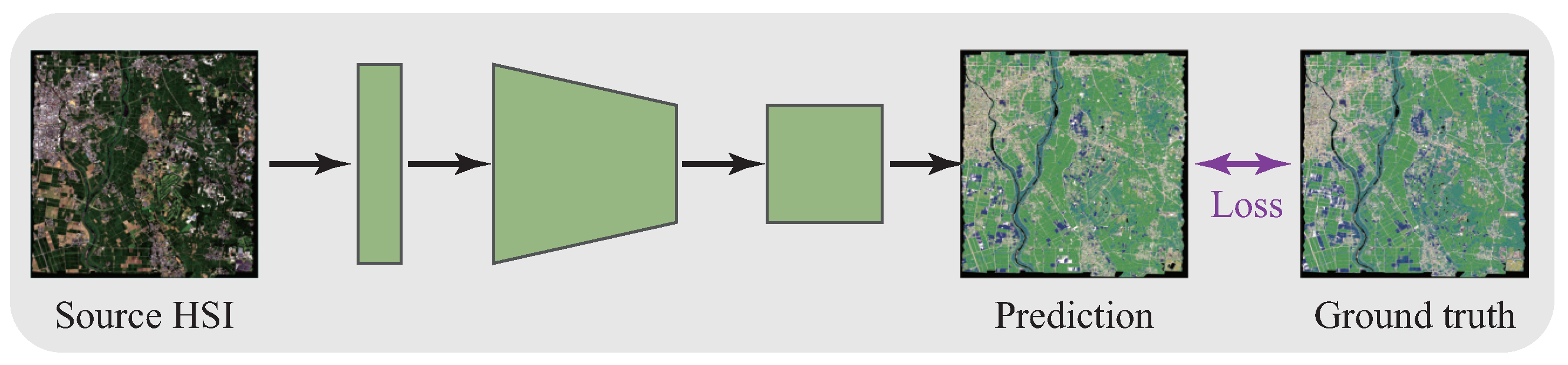
- (1)
- Pre-training on source HSIs (illustrated in Figure 1): Multiple different source HSIs are collected in advance, and multiple single-task models are fully trained on different source HSIs, respectively. Consequently, each model can acquire important information and knowledge from the corresponding hyperspectral domain.
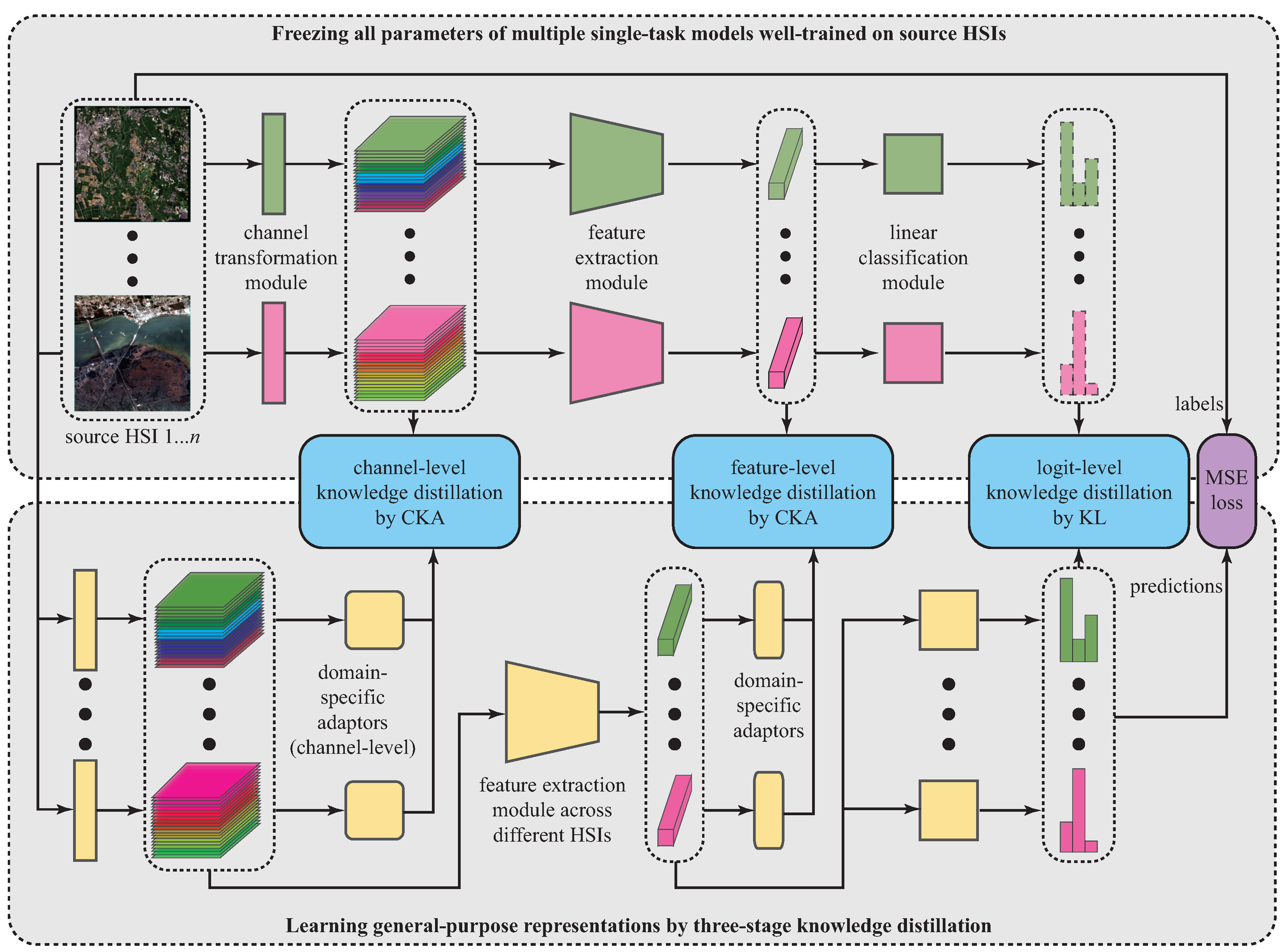
- (2)
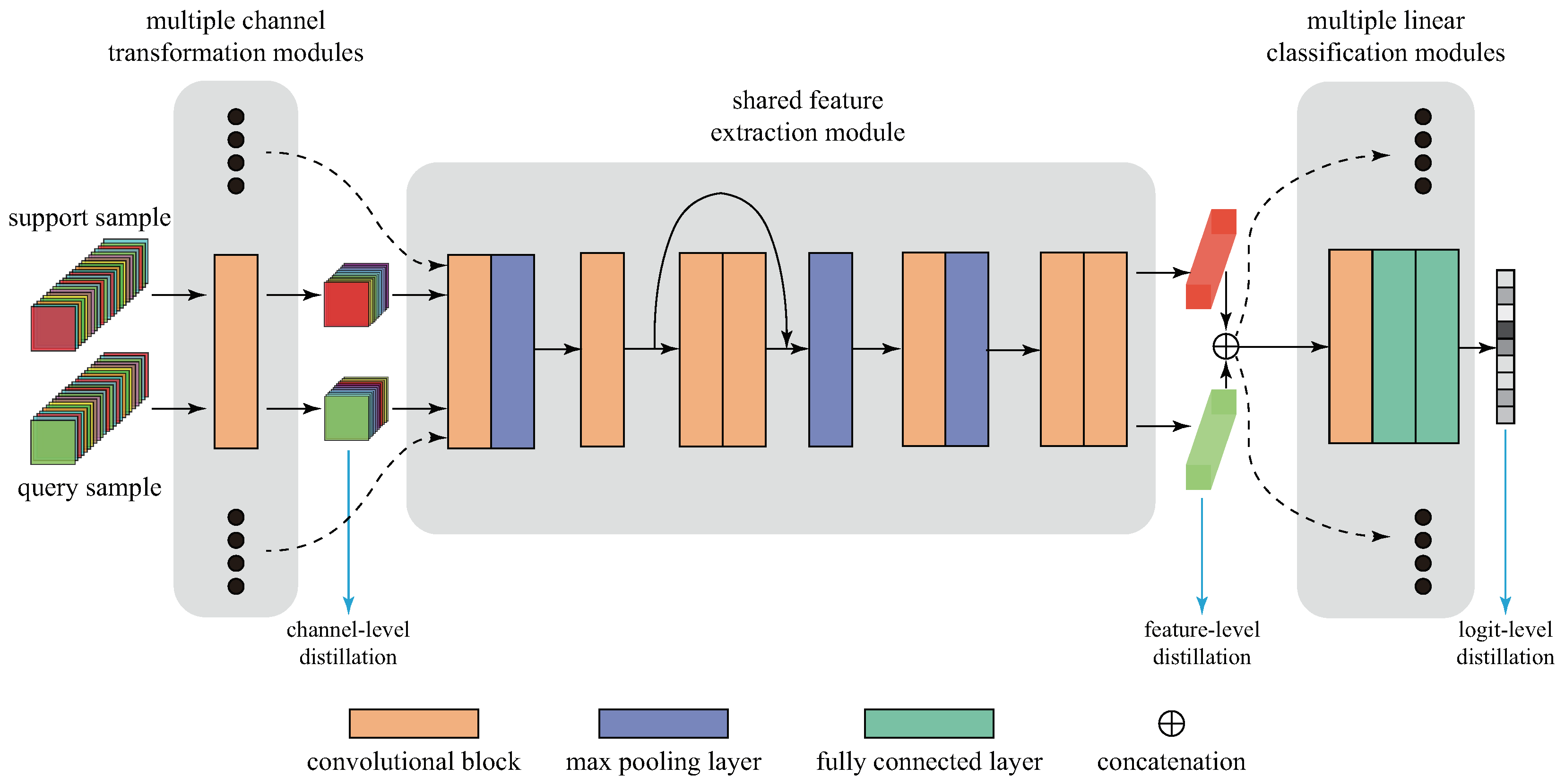
- Learning general-purpose representations (illustrated in Figure 2): All the parameters of the multiple single-task models well-trained on source HSIs are frozen, and the randomly initialized multi-task model is fully trained with the three-level distillation strategy and episode-based learning strategy to learn general-purpose representations from multiple different hyperspectral domains. In the designed multi-task model, the single feature extraction module is shared across different HSIs, while multiple channel transformation modules and linear classification modules are domain-specific (illustrated in the bottom half of Figure 2).
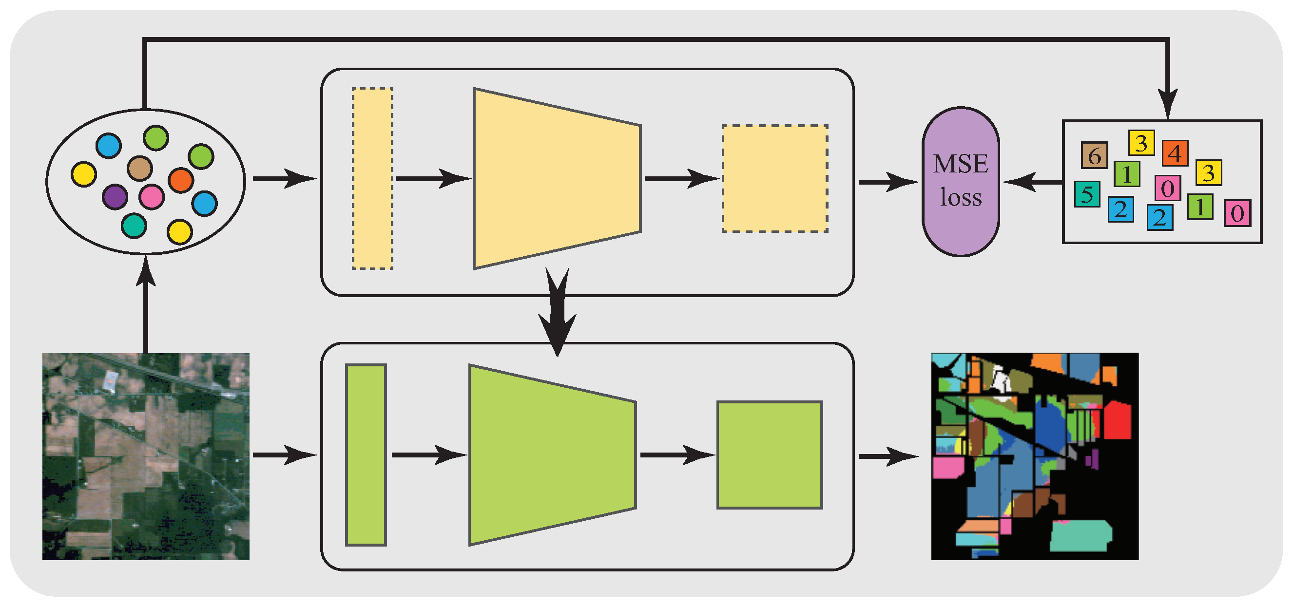
- (3)
- Fast adaption to target HSIs (illustrated in Figure 3): For each target HSI, only the feature extraction module well-trained in the previous step is inherited, while the channel transform module and the linear classification module are randomly initialized. Then, the whole model is fine-tuned using a few labeled samples to quickly adapt to the new hyperspectral domain.


3.2. Three-Level Knowledge Distillation
- (1)
- Domain-specific adaptors: The large difference between source HSIs means that the outputs of multiple single-task models can vary significantly, and the outputs of the multi-task model cannot match all of them simultaneously, whether at the channel level or feature level. Therefore, domain-specific adaptors are inserted (Figure 2) to map the outputs of the multi-task model into domain-specific vectors, which can be expressed as , where C, H and W are the number of channels, height and width, and and denote the inputs and outputs, respectively. In practice, the adaptor is instantiated with a 1×1 convolution layer with C kernels, and the difference between adaptors at the channel level and feature- evel is the value of C.
- (2)
- The CKA similarity index: Aligning features learned from substantially diverse domains requires a better and more complex distance function to model non-linear correlations between them. The calculation of CKA similarity can be divided into two steps. For the features and generated by the adopters of multi-task and single-task models, respectively, the radial basis function matrices and are first computed. Then, the similarity between them is measured as:where denotes the trace of a matrix, and denotes a centering matrix. In the training process, the alignment between high-dimensional features is achieved by minimizing .
3.3. Loss Function
3.4. Extensible Multi-Task Model
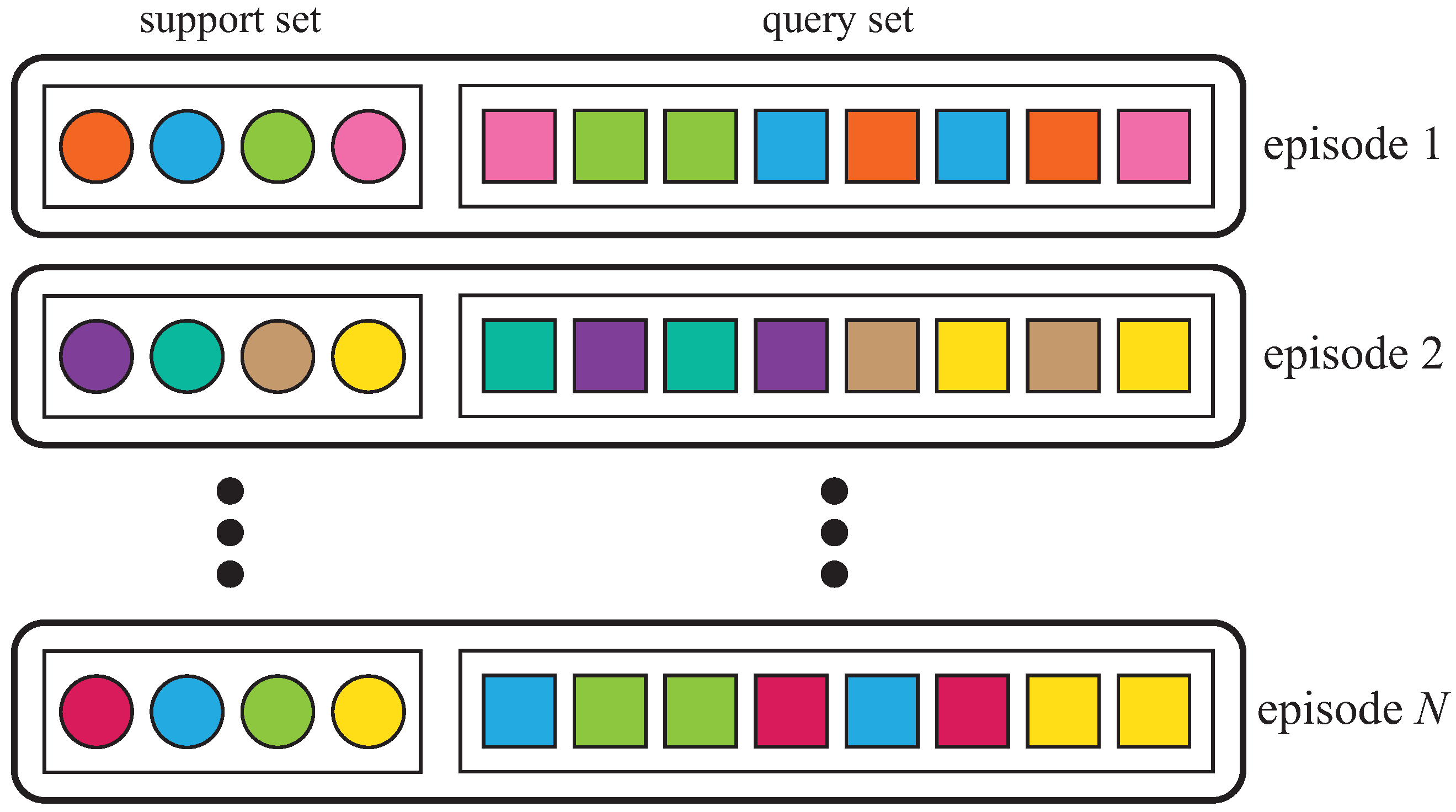
3.5. Episode-Based Learning Strategy
4. Experimental Results and Analysis
4.1. Data Sets
4.1.1. Source HSIs
4.1.2. Target HSIs
4.2. Environment and Settings
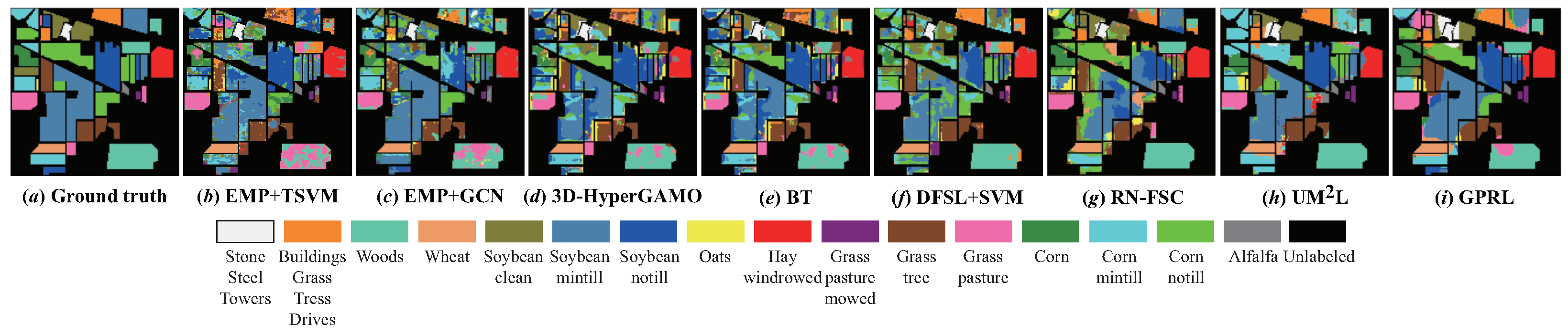
4.3. Classification Results and Analysis
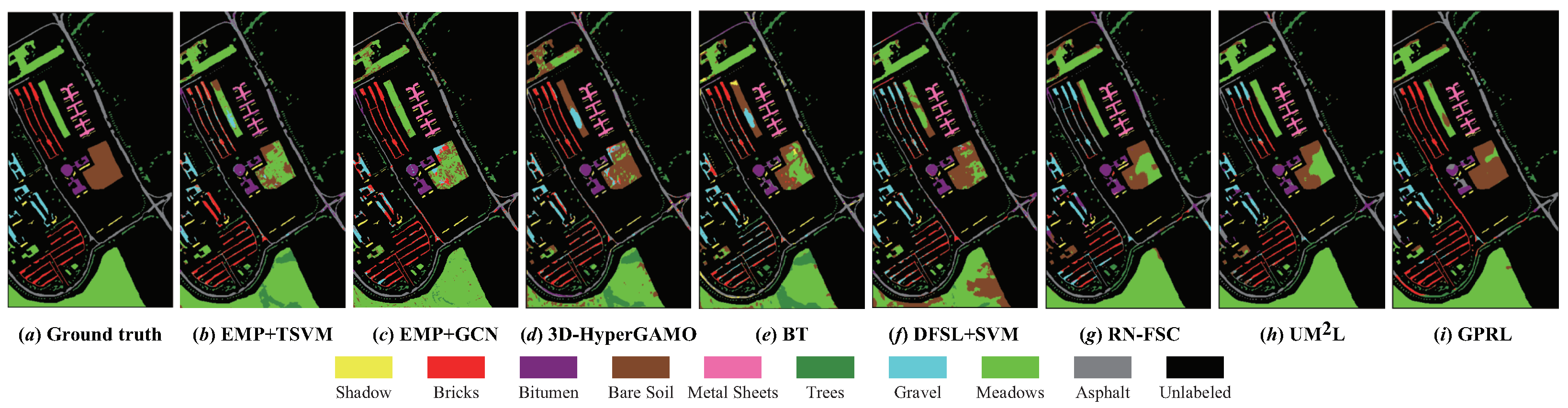
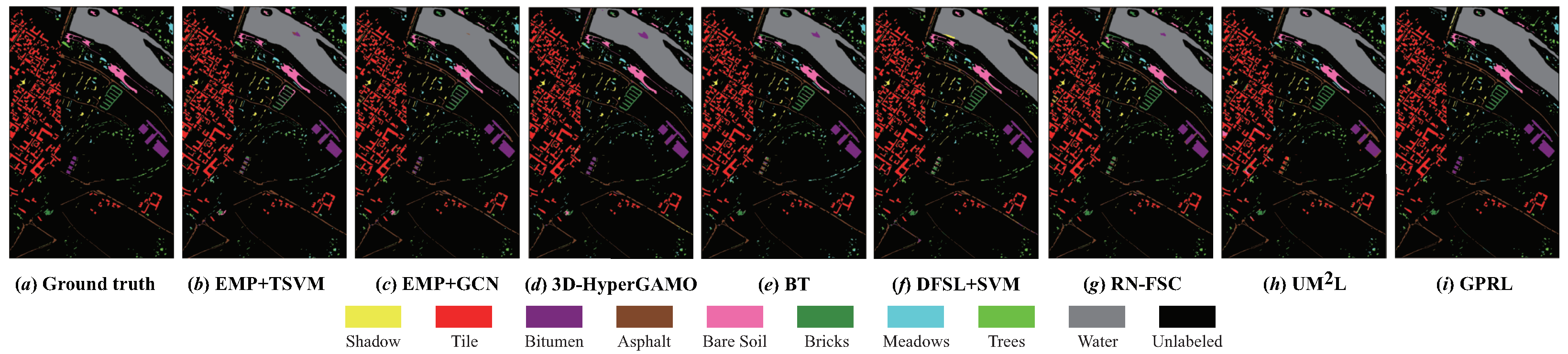
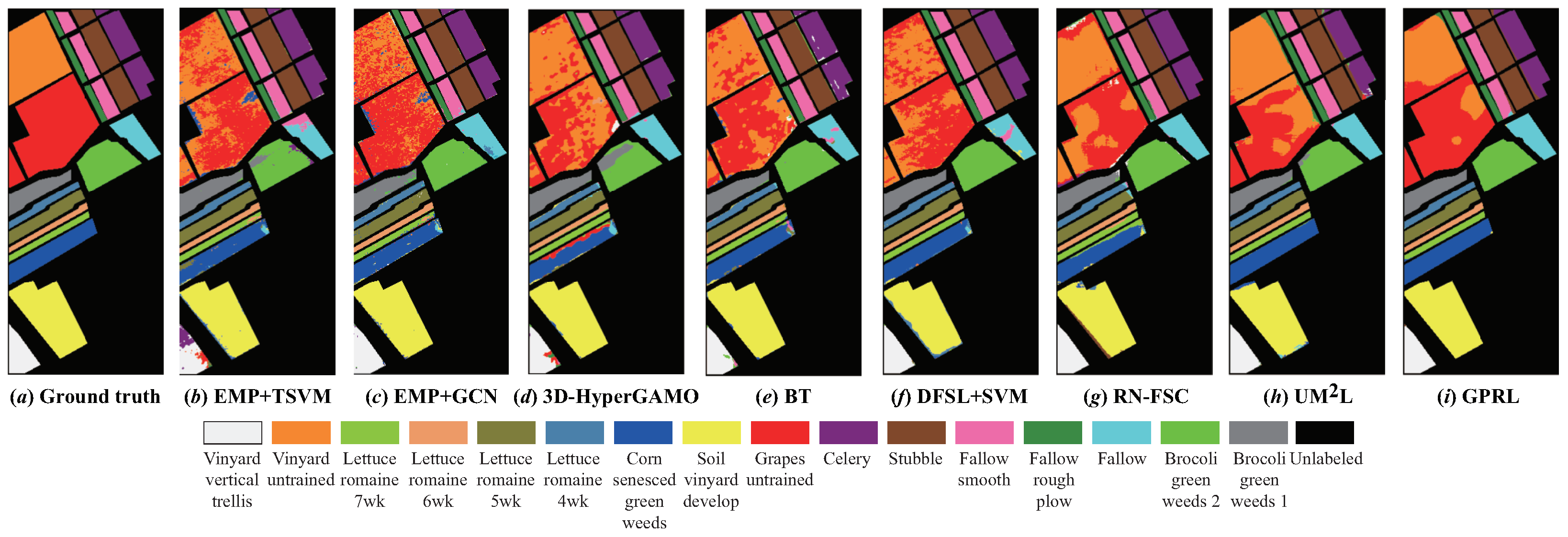
- (1)
- The traditional method (EMP+SVM) performs semi-supervised classification based on the extracted shallow EMP features and cannot make full use of the deep abstract features in HSIs, so its classification performance is significantly worse than that of other deep models.
- (2)
- The accuracy and robustness of the classification results of EMP+GCN, 3D-HyperGAMO and BT are obviously better than that of EMP+SVM. According to the OA, EMP+GCN has better performance on the UP and SA data sets, while 3D-HyperGAMO and BT can achieve better classification results on the PC and IP data sets, respectively. EMP+GCN and 3D-HyperGAMO can utilize unlabeled samples and synthetic samples, respectively, to assist model training on the target domain, and BT can utilize the more discriminative features in target HSIs, thus effectively improving the classification results.
- (3)
- The three cross-domain methods, DFSL+SVM, RN-FSC and UML, can further improve the performance of cross-domain HSI classification with samples. By using a large number of samples in the source HSIs to pre-train the deep models, the models can obtain a better initialization state compared with training from scratch so as to obtain higher classification accuracy in the target domains with small samples.
- (4)
- Obviously, the proposed method achieves the best classification results. For the four target HSIs, the OA of the proposed method is 3.52%, 0.56%, 2.47% and 0.62% higher than that of the second place, respectively, and the kappa coefficient of the proposed method is 4.78%, 0.80%, 2.73% and 0.66% higher than that of the second place, respectively. Compared with the other three cross-domain methods, on the one hand, the proposed method can learn more general-purpose representations from multiple-source domains with the three-level distillation strategy, and on the other hand, the proposed method trains the deep model based on the multi-task learning paradigm, which can better adapt to the characteristics of different target HSIs and make full use of the spatial–spectral information when only a few labeled samples are available.
4.4. General-Purpose Representations
4.4.1. From the Perspective of Classification Accuracy
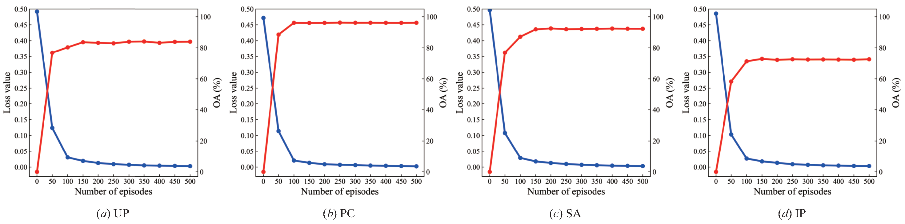
4.4.2. From the Perspective of Required Iterations
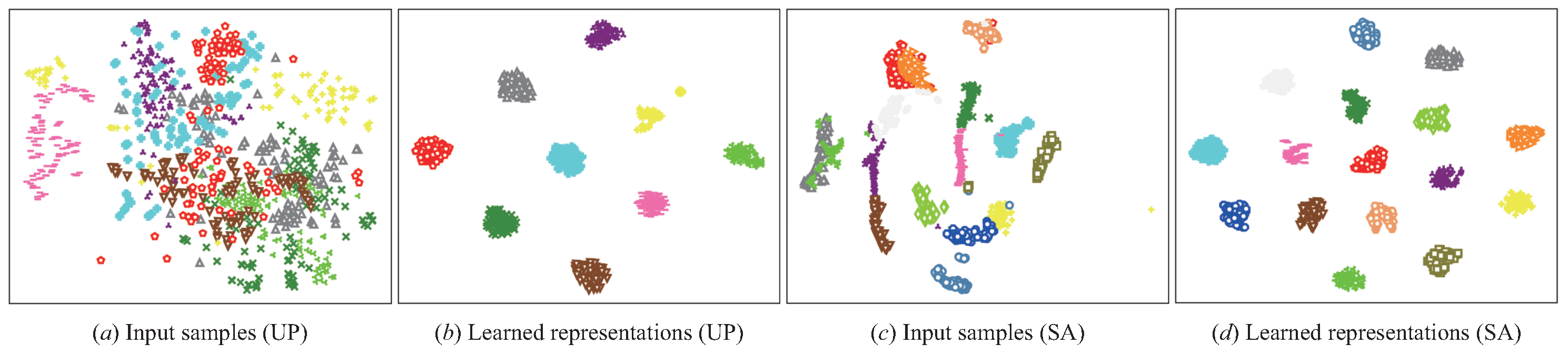
4.4.3. From the Perspective of Feature Separability
4.5. Hyperparameters Analysis
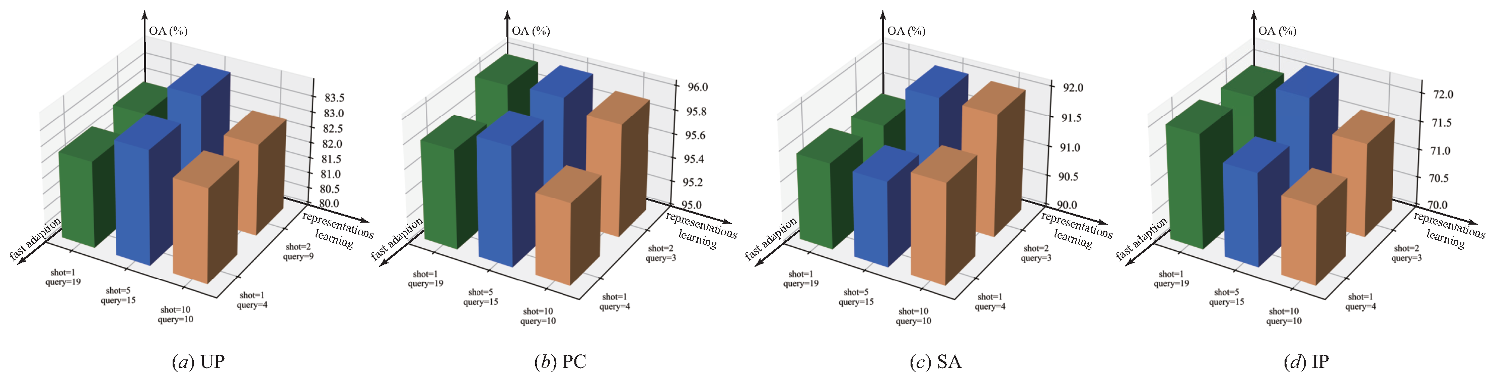
4.5.1. Episode Settings
4.5.2. The Level of Knowledge Distillation
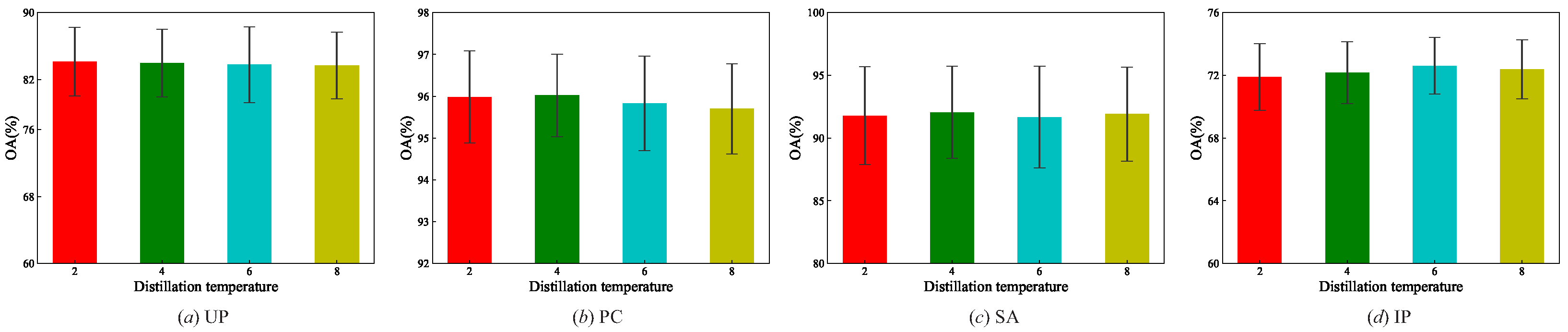
4.5.3. Distillation Temperature
4.5.4. Weight of Distillation Losses
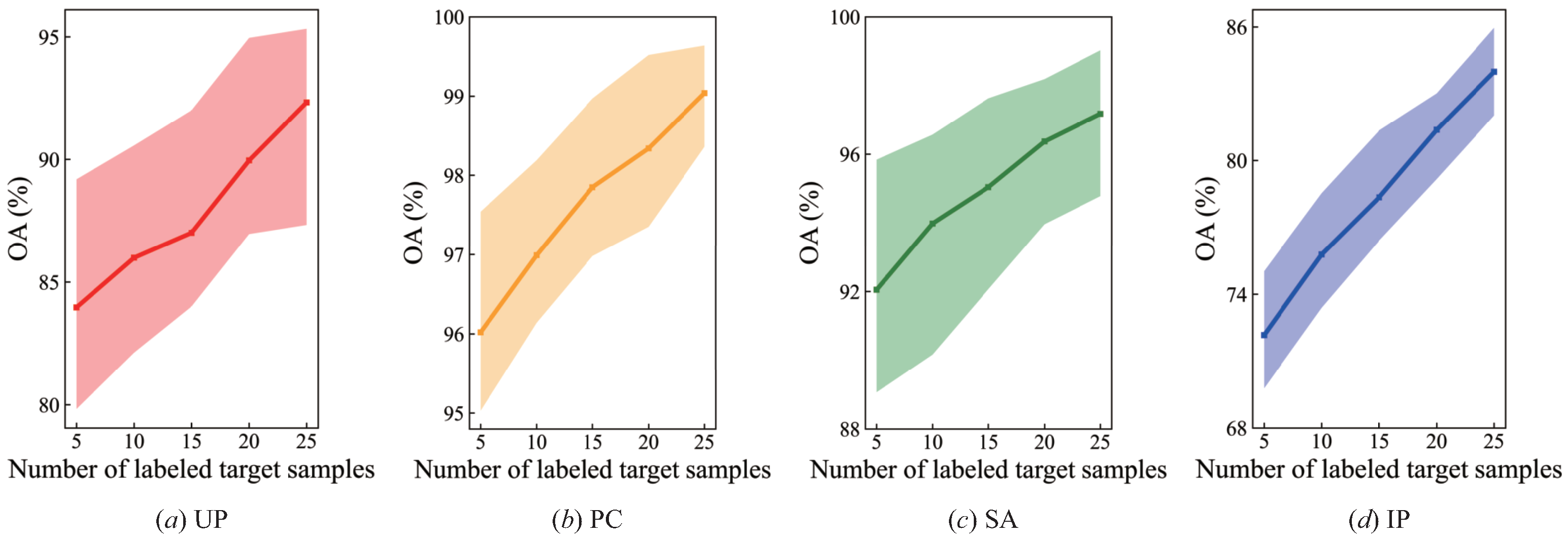
4.6. Influence of Labeled Target Samples
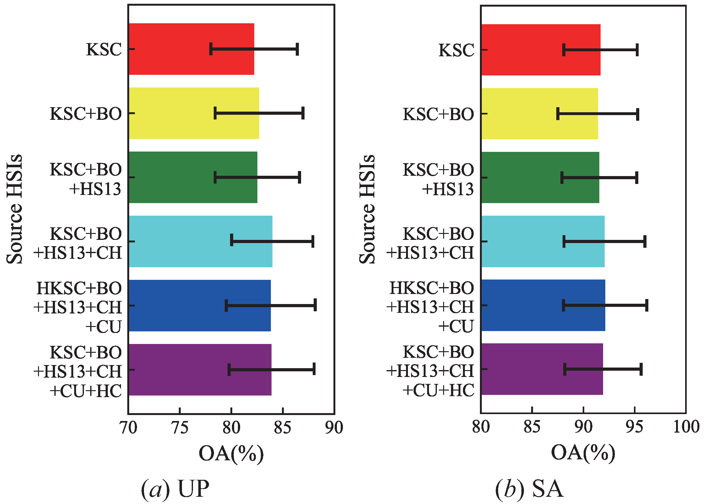
4.7. Influence of Different Source HSIs
4.8. Efficiency Analysis
5. Discussion and Future Work
Author Contributions
Funding
Institutional Review Board Statement
Informed Consent Statement
Data Availability Statement
Acknowledgments
Conflicts of Interest
References
- Xiao, J.; Li, J.; Yuan, Q.; Zhang, L. A Dual-UNet With Multistage Details Injection for Hyperspectral Image Fusion. IEEE Trans. Geosci. Remote Sens. 2022, 60, 5515313. [Google Scholar] [CrossRef]
- Booysen, R.; Lorenz, S.; Thiele, S.T.; Fuchsloch, W.C.; Marais, T.; Nex, P.A.; Gloaguen, R. Accurate hyperspectral imaging of mineralised outcrops: An example from lithium-bearing pegmatites at Uis, Namibia. Remote Sens. Environ. 2022, 269, 112790. [Google Scholar] [CrossRef]
- Liu, Z.; Zhong, Y.; Wang, X.; Shu, M.; Zhang, L. Unsupervised Deep Hyperspectral Video Target Tracking and High Spectral-Spatial-Temporal Resolution Benchmark Dataset. IEEE Trans. Geosci. Remote Sens. 2022, 60, 5513814. [Google Scholar] [CrossRef]
- Cui, Q.; Yang, B.; Liu, B.; Li, Y.; Ning, J. Tea Category Identification Using Wavelet Signal Reconstruction of Hyperspectral Imagery and Machine Learning. Agriculture 2022, 12, 1085. [Google Scholar] [CrossRef]
- Ghamisi, P.; Yokoya, N.; Li, J.; Liao, W.; Liu, S.; Plaza, J.; Rasti, B.; Plaza, A. Advances in Hyperspectral Image and Signal Processing: A Comprehensive Overview of the State of the Art. IEEE Geosci. Remote Sens. Mag. 2017, 5, 37–78. [Google Scholar] [CrossRef] [Green Version]
- Li, S.; Song, W.; Fang, L.; Chen, Y.; Ghamisi, P.; Benediktsson, J.A. Deep Learning for Hyperspectral Image Classification: An Overview. IEEE Trans. Geosci. Remote Sens. 2019, 57, 6690–6709. [Google Scholar] [CrossRef] [Green Version]
- Zhu, X.X.; Tuia, D.; Mou, L.; Xia, G.S.; Zhang, L.; Xu, F.; Fraundorfer, F. Deep Learning in Remote Sensing: A Comprehensive Review and List of Resources. IEEE Geosci. Remote Sens. Mag. 2017, 5, 8–36. [Google Scholar] [CrossRef] [Green Version]
- Paoletti, M.E.; Moreno-Álvarez, S.; Haut, J.M. Multiple Attention-Guided Capsule Networks for Hyperspectral Image Classification. IEEE Trans. Geosci. Remote Sens. 2022, 60, 5520420. [Google Scholar] [CrossRef]
- Mou, L.; Ghamisi, P.; Zhu, X.X. Deep Recurrent Neural Networks for Hyperspectral Image Classification. IEEE Trans. Geosci. Remote Sens. 2017, 55, 3639–3655. [Google Scholar] [CrossRef] [Green Version]
- Zhao, C.; Li, C.; Feng, S.; Li, W. Spectral–Spatial Anomaly Detection via Collaborative Representation Constraint Stacked Autoencoders for Hyperspectral Images. IEEE Geosci. Remote Sens. Lett. 2022, 19, 5503105. [Google Scholar] [CrossRef]
- Zhang, L.; Zhang, L. Artificial Intelligence for Remote Sensing Data Analysis: A review of challenges and opportunities. IEEE Geosci. Remote Sens. Mag. 2022, 10, 270–294. [Google Scholar] [CrossRef]
- Cheng, G.; Xie, X.; Han, J.; Guo, L.; Xia, G.S. Remote Sensing Image Scene Classification Meets Deep Learning: Challenges, Methods, Benchmarks, and Opportunities. IEEE J. Sel. Top. Appl. Earth Obs. Remote Sens. 2020, 13, 3735–3756. [Google Scholar] [CrossRef]
- Rasti, B.; Hong, D.; Hang, R.; Ghamisi, P.; Kang, X.; Chanussot, J.; Benediktsson, J.A. Feature Extraction for Hyperspectral Imagery: The Evolution From Shallow to Deep: Overview and Toolbox. IEEE Geosci. Remote Sens. Mag. 2020, 8, 60–88. [Google Scholar] [CrossRef]
- Liu, B.; Yu, X.; Yu, A.; Zhang, P.; Wan, G.; Wang, R. Deep Few-Shot Learning for Hyperspectral Image Classification. IEEE Trans. Geosci. Remote Sens. 2019, 57, 2290–2304. [Google Scholar] [CrossRef]
- Gao, K.; Liu, B.; Yu, X.; Qin, J.; Zhang, P.; Tan, X. Deep Relation Network for Hyperspectral Image Few-Shot Classification. Remote Sens. 2020, 12, 923. [Google Scholar] [CrossRef] [Green Version]
- Lee, H.; Eum, S.; Kwon, H. Exploring Cross-Domain Pretrained Model for Hyperspectral Image Classification. IEEE Trans. Geosci. Remote Sens. 2022, 60, 5526812. [Google Scholar] [CrossRef]
- Ma, X.; Mou, X.; Wang, J.; Liu, X.; Wang, H.; Yin, B. Cross-Data Set Hyperspectral Image Classification Based on Deep Domain Adaptation. IEEE Trans. Geosci. Remote Sens. 2019, 57, 10164–10174. [Google Scholar] [CrossRef]
- Ma, X.; Mou, X.; Wang, J.; Liu, X.; Geng, J.; Wang, H. Cross-Dataset Hyperspectral Image Classification Based on Adversarial Domain Adaptation. IEEE Trans. Geosci. Remote Sens. 2021, 59, 4179–4190. [Google Scholar] [CrossRef]
- Qin, Y.; Bruzzone, L.; Li, B.; Ye, Y. Cross-Domain Collaborative Learning via Cluster Canonical Correlation Analysis and Random Walker for Hyperspectral Image Classification. IEEE Trans. Geosci. Remote Sens. 2019, 57, 3952–3966. [Google Scholar] [CrossRef] [Green Version]
- Zhang, C.; Ye, M.; Lei, L.; Qian, Y. Feature Selection for Cross-Scene Hyperspectral Image Classification Using Cross-Domain I-ReliefF. IEEE J. Sel. Top. Appl. Earth Obs. Remote Sens. 2021, 14, 5932–5949. [Google Scholar] [CrossRef]
- Shen, J.; Cao, X.; Li, Y.; Xu, D. Feature Adaptation and Augmentation for Cross-Scene Hyperspectral Image Classification. IEEE Geosci. Remote Sens. Lett. 2018, 15, 622–626. [Google Scholar] [CrossRef]
- Miao, J.; Zhang, B.; Wang, B. Coarse-to-Fine Joint Distribution Alignment for Cross-Domain Hyperspectral Image Classification. IEEE J. Sel. Top. Appl. Earth Obs. Remote Sens. 2021, 14, 12415–12428. [Google Scholar] [CrossRef]
- Chen, Y.; Jiang, H.; Li, C.; Jia, X.; Ghamisi, P. Deep Feature Extraction and Classification of Hyperspectral Images Based on Convolutional Neural Networks. IEEE Trans. Geosci. Remote Sens. 2016, 54, 6232–6251. [Google Scholar] [CrossRef] [Green Version]
- Zhong, Y.; Hu, X.; Luo, C.; Wang, X.; Zhao, J.; Zhang, L. WHU-Hi: UAV-borne hyperspectral with high spatial resolution (H2) benchmark datasets and classifier for precise crop identification based on deep convolutional neural network with CRF. Remote Sens. Environ. 2020, 250, 112012. [Google Scholar] [CrossRef]
- Gao, K.; Liu, B.; Yu, X.; Yu, A. Unsupervised Meta Learning With Multiview Constraints for Hyperspectral Image Small Sample set Classification. IEEE Trans. Image Process. 2022, 31, 3449–3462. [Google Scholar] [CrossRef]
- Paoletti, M.E.; Haut, J.M.; Tao, X.; Plaza, J.; Plaza, A. FLOP-Reduction Through Memory Allocations Within CNN for Hyperspectral Image Classification. IEEE Trans. Geosci. Remote Sens. 2021, 59, 5938–5952. [Google Scholar] [CrossRef]
- Liu, B.; Yu, X.; Zhang, P.; Yu, A.; Fu, Q.; Wei, X. Supervised Deep Feature Extraction for Hyperspectral Image Classification. IEEE Trans. Geosci. Remote Sens. 2018, 56, 1909–1921. [Google Scholar] [CrossRef]
- Gao, K.; Guo, W.; Yu, X.; Liu, B.; Yu, A.; Wei, X. Deep Induction Network for Small Samples Classification of Hyperspectral Images. IEEE J. Sel. Top. Appl. Earth Obs. Remote Sens. 2020, 13, 3462–3477. [Google Scholar] [CrossRef]
- Xue, Z.; Yu, X.; Tan, X.; Liu, B.; Yu, A.; Wei, X. Multiscale Deep Learning Network With Self-Calibrated Convolution for Hyperspectral and LiDAR Data Collaborative Classification. IEEE Trans. Geosci. Remote Sens. 2022, 60, 5514116. [Google Scholar] [CrossRef]
- Tan, X.; Gao, K.; Liu, B.; Fu, Y.; Kang, L. Deep global-local transformer network combined with extended morphological profiles for hyperspectral image classification. J. Appl. Remote Sens. 2021, 15, 038509. [Google Scholar] [CrossRef]
- Xu, Q.; Wang, D.; Luo, B. Faster Multiscale Capsule Network With Octave Convolution for Hyperspectral Image Classification. IEEE Geosci. Remote Sens. Lett. 2021, 18, 361–365. [Google Scholar] [CrossRef]
- Liu, B.; Gao, K.; Yu, A.; Guo, W.; Wang, R.; Zuo, X. Semisupervised graph convolutional network for hyperspectral image classification. J. Appl. Remote Sens. 2020, 14, 026516. [Google Scholar] [CrossRef]
- Wan, S.; Pan, S.; Zhong, P.; Chang, X.; Yang, J.; Gong, C. Dual Interactive Graph Convolutional Networks for Hyperspectral Image Classification. IEEE Trans. Geosci. Remote Sens. 2022, 60, 5510214. [Google Scholar] [CrossRef]
- He, X.; Chen, Y. Transferring CNN Ensemble for Hyperspectral Image Classification. IEEE Geosci. Remote Sens. Lett. 2021, 18, 876–880. [Google Scholar] [CrossRef]
- He, X.; Chen, Y.; Ghamisi, P. Heterogeneous Transfer Learning for Hyperspectral Image Classification Based on Convolutional Neural Network. IEEE Trans. Geosci. Remote Sens. 2020, 58, 3246–3263. [Google Scholar] [CrossRef]
- Liu, B.; Yu, A.; Yu, X.; Wang, R.; Gao, K.; Guo, W. Deep Multiview Learning for Hyperspectral Image Classification. IEEE Trans. Geosci. Remote Sens. 2021, 59, 7758–7772. [Google Scholar] [CrossRef]
- Hou, S.; Shi, H.; Cao, X.; Zhang, X.; Jiao, L. Hyperspectral Imagery Classification Based on Contrastive Learning. IEEE Trans. Geosci. Remote Sens. 2022, 60, 5521213. [Google Scholar] [CrossRef]
- Gou, J.; Yu, B.; Maybank, S.J.; Tao, D. Knowledge Distillation: A Survey. Int. J. Comput. Vis. 2021, 129, 1789–1819. [Google Scholar] [CrossRef]
- Li, W.; Liu, X.; Bilen, H. Universal Representations: A Unified Look at Multiple Task and Domain Learning. arXiv 2022. [Google Scholar] [CrossRef]
- Hinton, G.E.; Vinyals, O.; Dean, J. Distilling the Knowledge in a Neural Network. arXiv 2015, arXiv:1503.02531. [Google Scholar]
- Romero, A.; Ballas, N.; Kahou, S.E.; Chassang, A.; Gatta, C.; Bengio, Y. FitNets: Hints for Thin Deep Nets. arXiv 2014, arXiv:1412.6550. [Google Scholar]
- Zagoruyko, S.; Komodakis, N. Paying More Attention to Attention: Improving the Performance of Convolutional Neural Networks via Attention Transfer. arXiv 2016, arXiv:1612.03928. [Google Scholar]
- Yim, J.; Joo, D.; Bae, J.; Kim, J. A Gift from Knowledge Distillation: Fast Optimization, Network Minimization and Transfer Learning. In Proceedings of the 2017 IEEE Conference on Computer Vision and Pattern Recognition (CVPR), Honolulu, HI, USA, 21–26 July 2017; pp. 7130–7138. [Google Scholar] [CrossRef]
- Li, W.H.; Bilen, H. Knowledge Distillation for Multi-task Learning. In Proceedings of the Computer Vision—ECCV 2020 Workshops; Bartoli, A., Fusiello, A., Eds.; Springer International Publishing: Cham, Switzerland, 2020; pp. 163–176. [Google Scholar]
- Shi, C.; Fang, L.; Lv, Z.; Zhao, M. Explainable scale distillation for hyperspectral image classification. Pattern Recognit. 2022, 122, 108316. [Google Scholar] [CrossRef]
- Yue, J.; Fang, L.; Rahmani, H.; Ghamisi, P. Self-Supervised Learning With Adaptive Distillation for Hyperspectral Image Classification. IEEE Trans. Geosci. Remote Sensing 2022, 60, 5501813. [Google Scholar] [CrossRef]
- Finn, C.; Abbeel, P.; Levine, S. Model-Agnostic Meta-Learning for Fast Adaptation of Deep Networks. arXiv 2017, arXiv:1703.03400. [Google Scholar]
- Snell, J.; Swersky, K.; Zemel, R. Prototypical Networks for Few-shot Learning. arXiv 2017, arXiv:1703.05175. [Google Scholar]
- Sung, F.; Yang, Y.; Zhang, L.; Xiang, T.; Torr, P.; Hospedales, T. Learning to Compare: Relation Network for Few-Shot Learning. In Proceedings of the 2018 IEEE/CVF Conference on Computer Vision and Pattern Recognition, Salt Lake City, UT, USA, 18–23 June 2018; pp. 1199–1208. [Google Scholar] [CrossRef] [Green Version]
- Geng, R.; Li, B.; Li, Y.; Zhu, X.; Jian, P.; Sun, J. Induction Networks for Few-Shot Text Classification. In Proceedings of the 2019 Conference on Empirical Methods in Natural Language Processing and the 9th International Joint Conference on Natural Language Processing (EMNLP-IJCNLP); Association for Computational Linguistics: Hong Kong, China, 2019. [Google Scholar] [CrossRef] [Green Version]
- Gao, K.; Liu, B.; Yu, X.; Zhang, P.; Tan, X.; Sun, Y. Small sample classification of hyperspectral image using model-agnostic meta-learning algorithm and convolutional neural network. Int. J. Remote Sens. 2021, 42, 3090–3122. [Google Scholar] [CrossRef]
- Ma, X.; Ji, S.; Wang, J.; Geng, J.; Wang, H. Hyperspectral Image Classification Based on Two-Phase Relation Learning Network. IEEE Trans. Geosci. Remote Sens. 2019, 57, 10398–10409. [Google Scholar] [CrossRef]
- Motiian, S.; Jones, Q.; Iranmanesh, S.M.; Doretto, G. Few-Shot Adversarial Domain Adaptation. In Proceedings of the Advances in Neural Information Processing Systems 30: Annual Conference on Neural Information Processing Systems 2017, Long Beach, CA, USA, 4–9 December 2017; Guyon, I., von Luxburg, U., Bengio, S., Wallach, H.M., Fergus, R., Vishwanathan, S.V.N., Garnett, R., Eds.; pp. 6670–6680. [Google Scholar]
- Bi, H.; Liu, Z.; Deng, J.; Ji, Z.; Zhang, J. Contrastive Domain Adaptation-Based Sparse SAR Target Classification under Few-Shot Cases. Remote Sens. 2023, 15, 469. [Google Scholar] [CrossRef]
- Rostami, M.; Kolouri, S.; Eaton, E.; Kim, K. Deep Transfer Learning for Few-Shot SAR Image Classification. Remote Sens. 2019, 11, 1374. [Google Scholar] [CrossRef] [Green Version]
- Lasloum, T.; Alhichri, H.; Bazi, Y.; Alajlan, N. SSDAN: Multi-Source Semi-Supervised Domain Adaptation Network for Remote Sensing Scene Classification. Remote Sens. 2021, 13, 3861. [Google Scholar] [CrossRef]
- Shi, Y.; Li, J.; Li, Y.; Du, Q. Sensor-Independent Hyperspectral Target Detection With Semisupervised Domain Adaptive Few-Shot Learning. IEEE Trans. Geosci. Remote Sens. 2021, 59, 6894–6906. [Google Scholar] [CrossRef]
- Wang, L.; Hao, S.; Wang, Q.; Wang, Y. Semi-supervised classification for hyperspectral imagery based on spatial-spectral Label Propagation. ISPRS J. Photogramm. Remote Sens. 2014, 97, 123–137. [Google Scholar] [CrossRef]
- Roy, S.K.; Haut, J.M.; Paoletti, M.E.; Dubey, S.R.; Plaza, A. Generative Adversarial Minority Oversampling for Spectral–Spatial Hyperspectral Image Classification. IEEE Trans. Geosci. Remote Sens. 2022, 60, 5500615. [Google Scholar] [CrossRef]
- Zbontar, J.; Jing, L.; Misra, I.; LeCun, Y.; Deny, S. Barlow Twins: Self-Supervised Learning via Redundancy Reduction. In Proceedings of the 38th International Conference on Machine Learning, ICML 2021, Virtual Event, 18–24 July 2021; Meila, M., Zhang, T., Eds.; Volume 139, pp. 12310–12320. [Google Scholar]
- van der Maaten, L.; Hinton, G. Viualizing data using t-SNE. J. Mach. Learn. Res. 2008, 9, 2579–2605. [Google Scholar]


| Source HSIs | Target HSIs | |||||||||
|---|---|---|---|---|---|---|---|---|---|---|
| HC | CU | HS13 | BO | KSC | CH | UP | PC | SA | IP | |
| Spatial size | 1217 × 303 | 614 × 512 | 349 × 1905 | 1476 × 256 | 512 × 614 | 2517 × 2335 | 610 × 340 | 1096 × 715 | 512 × 217 | 145 × 145 |
| Spectral range | 400–1000 | 370–2480 | 380–1050 | 400–2500 | 400–2500 | 363–1018 | 430–860 | 430–860 | 400–2500 | 400–2500 |
| No. of bands | 274 | 190 | 144 | 145 | 176 | 128 | 103 | 102 | 204 | 200 |
| GSD | 0.109 | 20 | 2.5 | 30 | 18 | 2.5 | 1.3 | 1.3 | 3.7 | 20 |
| Sensor type | Headwall Nano- Hyperspec | AVIRIS | ITRES- CASI 1500 | EO-1 | AVIRIS | Hyperspec -VNIR-C | ROSIS | ROSIS | AVIRIS | AVIRIS |
| Areas | HanChuan | Cuprite | Houston | Botswana | Florida | Chikusei | Pavia | Pavia | California | Indiana |
| No. of classes | 16 | 8 | 15 | 14 | 13 | 19 | 9 | 9 | 16 | 16 |
| Total labeled samples | 257,530 | 3837 | 15,029 | 3248 | 5211 | 77,592 | 42,776 | 148,152 | 54,129 | 10,249 |
| Labeled samples for training | 200 per class | 5 per class | ||||||||
| HSI | Criteria | EMP+TSVM | EMP+GCN | 3D-HyperGAMO | BT | DFSL+SVM | RN-FSC | UML | GPRL |
|---|---|---|---|---|---|---|---|---|---|
| Mean ± SD | Mean ± SD | Mean ± SD | Mean ± SD | Mean ± SD | Mean ± SD | Mean ± SD | Mean ± SD | ||
| UP | OA | 69.58 ± 7.55 | 75.23 ± 3.96 | 70.42 ± 4.91 | 70.03 ± 3.09 | 71.64 ± 6.07 | 77.16 ± 5.82 | 80.49 ± 3.64 | 84.01 ± 4.31 |
| AA | 72.65 ± 3.70 | 75.12 ± 3.27 | 69.97 ± 3.60 | 69.63 ± 2.84 | 74.12 ± 4.65 | 72.60 ± 4.38 | 77.79 ± 3.05 | 82.32 ± 2.99 | |
| kappa | 61.83 ± 7.67 | 68.02 ± 4.19 | 62.59 ± 5.45 | 62.40 ± 3.51 | 64.41 ± 6.53 | 70.86 ± 6.66 | 74.70 ± 4.05 | 79.48 ± 5.14 | |
| PC | OA | 92.83 ± 1.90 | 95.01 ± 0.83 | 95.27 ± 2.23 | 95.19 ± 2.37 | 95.54 ± 1.52 | 95.61 ± 1.08 | 94.43 ± 1.12 | 96.17 ± 0.74 |
| AA | 83.01 ± 2.77 | 85.43 ± 1.68 | 86.61 ± 4.62 | 86.53 ± 4.85 | 87.27 ± 2.59 | 88.14 ± 1.82 | 84.89 ± 2.61 | 89.00 ± 2.30 | |
| kappa | 89.96 ± 2.57 | 92.98 ± 1.16 | 93.35 ± 3.08 | 93.20 ± 3.22 | 93.75 ± 2.04 | 93.79 ± 1.52 | 92.17 ± 1.56 | 94.59 ± 1.04 | |
| SA | OA | 83.58 ± 1.65 | 85.93 ± 0.99 | 83.70 ± 4.40 | 83.70 ± 4.17 | 84.52 ± 3.32 | 86.37 ± 3.32 | 89.82 ± 4.18 | 92.29 ± 3.55 |
| AA | 87.54 ± 0.79 | 89.87 ± 0.98 | 88.76 ± 2.59 | 86.62 ± 2.49 | 91.67 ± 0.84 | 89.75 ± 1.61 | 92.99 ± 2.23 | 95.15 ± 1.76 | |
| kappa | 81.78 ± 1.81 | 84.33 ± 1.10 | 81.97 ± 4.84 | 81.98 ± 4.59 | 82.90 ± 3.60 | 84.91 ± 3.65 | 88.72 ± 4.61 | 91.45 ± 3.92 | |
| IP | OA | 55.09 ± 3.51 | 55.98 ± 2.93 | 57.02 ± 3.00 | 58.36 ± 2.39 | 60.18 ± 3.53 | 60.84 ± 3.15 | 71.65 ± 2.17 | 72.27 ± 2.61 |
| AA | 55.19 ± 1.96 | 54.77 ± 1.89 | 55.48 ± 2.47 | 52.86 ± 1.96 | 59.41 ± 1.73 | 56.66 ± 4.65 | 64.60 ± 2.74 | 65.26 ± 2.56 | |
| kappa | 49.62 ± 3.80 | 50.65 ± 3.00 | 52.17 ± 3.30 | 54.37 ± 2.50 | 55.66 ± 3.72 | 56.52 ± 3.41 | 68.29 ± 2.35 | 68.95 ± 2.88 |
| HSI | Criteria | Baseline | Baseline + Meta-Training | Baseline + Meta-Training + Knowledge Distillation |
|---|---|---|---|---|
| Mean ± SD | Mean ± SD | Mean ± SD | ||
| UP | OA | 78.73 ± 3.00 | 80.84 ± 3.88 | 84.01 ± 4.31 |
| AA | 77.85 ± 2.86 | 78.48 ± 2.39 | 82.32 ± 2.99 | |
| kappa | 72.86 ± 3.36 | 75.56 ± 4.57 | 79.48 ± 5.14 | |
| PC | OA | 94.54 ± 1.01 | 95.19 ± 0.77 | 96.17 ± 0.74 |
| AA | 86.07 ± 2.35 | 86.37 ± 2.09 | 89.00 ± 2.30 | |
| kappa | 92.33 ± 1.39 | 93.21 ± 1.08 | 94.59 ± 1.04 | |
| SA | OA | 89.45 ± 3.78 | 90.97 ± 4.07 | 92.29 ± 3.55 |
| AA | 93.90 ± 1.73 | 94.18 ± 1.90 | 95.15 ± 1.76 | |
| kappa | 88.32 ± 4.16 | 90.00 ± 4.48 | 91.45 ± 3.92 | |
| IP | OA | 67.29 ± 1.53 | 69.27 ± 4.85 | 72.27 ± 2.61 |
| AA | 66.00 ± 3.99 | 62.42 ± 3.90 | 65.26 ± 2.56 | |
| kappa | 63.42 ± 1.65 | 65.82 ± 5.11 | 68.95 ± 2.88 |
| HSI | Criteria | F | F + C | F + L | F + C + L |
|---|---|---|---|---|---|
| Mean ± SD | Mean ± SD | Mean ± SD | Mean ± SD | ||
| UP | OA | 82.94 ± 4.17 | 83.20 ± 3.43 | 83.70 ± 4.19 | 84.01 ± 4.31 |
| AA | 81.31 ± 2.16 | 80.50 ± 2.58 | 81.43 ± 2.75 | 82.32 ± 2.99 | |
| kappa | 78.16 ± 4.80 | 78.40 ± 4.07 | 79.06 ± 4.98 | 79.48 ± 5.14 | |
| PC | OA | 95.23 ± 0.96 | 95.55 ± 1.01 | 95.75 ± 0.89 | 96.17 ± 0.74 |
| AA | 86.93 ± 2.39 | 87.86 ± 1.74 | 88.27 ± 1.73 | 89.00 ± 2.30 | |
| kappa | 93.28 ± 1.34 | 93.71 ± 1.43 | 93.98 ± 1.26 | 94.59 ± 1.04 | |
| SA | OA | 91.20 ± 3.94 | 91.15 ± 3.77 | 91.67 ± 4.03 | 92.29 ± 3.55 |
| AA | 94.12 ± 1.91 | 93.96 ± 1.91 | 94.86 ± 1.92 | 95.15 ± 1.76 | |
| kappa | 90.25 ± 4.34 | 90.19 ± 4.16 | 90.77 ± 4.44 | 91.45 ± 3.92 | |
| IP | OA | 71.31 ± 1.94 | 71.79 ± 2.96 | 72.07 ± 2.47 | 72.27 ± 2.61 |
| AA | 65.21 ± 3.67 | 66.22 ± 2.80 | 65.63 ± 4.32 | 65.26 ± 2.56 | |
| kappa | 67.94 ± 2.17 | 68.48 ± 3.09 | 68.77 ± 2.63 | 68.95 ± 2.88 |
| HSI | Criteria | = 0.4 | = 0.6 | = 0.8 | = 1.0 |
|---|---|---|---|---|---|
| Mean ± SD | Mean ± SD | Mean ± SD | Mean ± SD | ||
| UP | OA | 81.87 ± 4.03 | 83.03 ± 3.63 | 84.01 ± 4.31 | 83.97 ± 4.10 |
| AA | 79.34 ± 2.52 | 80.30 ± 2.97 | 82.32 ± 2.99 | 82.47 ± 1.33 | |
| kappa | 76.79 ± 4.96 | 78.16 ± 4.25 | 79.48 ± 5.14 | 79.46 ± 4.83 | |
| PC | OA | 95.30 ± 0.97 | 95.75 ± 0.99 | 96.17 ± 0.74 | 96.02 ± 0.99 |
| AA | 86.97 ± 2.41 | 88.03 ± 1.66 | 89.00 ± 2.30 | 88.42 ± 2.16 | |
| kappa | 93.36 ± 1.39 | 93.79 ± 1.50 | 94.59 ± 1.04 | 94.37 ± 1.40 | |
| SA | OA | 91.00 ± 3.98 | 91.63 ± 3.83 | 92.29 ± 3.55 | 92.05 ± 3.66 |
| AA | 94.01 ± 1.93 | 94.42 ± 1.97 | 95.15 ± 1.76 | 94.58 ± 1.91 | |
| kappa | 90.07 ± 4.41 | 90.65 ± 4.26 | 91.45 ± 3.92 | 91.19 ± 4.04 | |
| IP | OA | 70.18 ± 1.96 | 71.53 ± 2.77 | 72.27 ± 2.61 | 72.17 ± 1.80 |
| AA | 64.19 ± 3.52 | 66.04 ± 2.53 | 65.26 ± 2.56 | 66.04 ± 3.57 | |
| kappa | 66.96 ± 2.30 | 68.29 ± 2.99 | 68.95 ± 2.88 | 68.79 ± 2.09 |
| Phases | DFSL + SVM | RN-FSC | UML | GPRL |
|---|---|---|---|---|
| Pre-training | 118.23 min | 319.84 min | 316.87 min | 15.01 min |
| Knowledge distillation | / | / | / | 37.64 min |
| Fine-tuning | 9.15 s | 80.47 s | 363.32 s | 32.93 s |
| Classification | 1.88 s | 19.12 s | 141.83 s | 13.37 s |
Disclaimer/Publisher’s Note: The statements, opinions and data contained in all publications are solely those of the individual author(s) and contributor(s) and not of MDPI and/or the editor(s). MDPI and/or the editor(s) disclaim responsibility for any injury to people or property resulting from any ideas, methods, instructions or products referred to in the content. |
© 2023 by the authors. Licensee MDPI, Basel, Switzerland. This article is an open access article distributed under the terms and conditions of the Creative Commons Attribution (CC BY) license (https://creativecommons.org/licenses/by/4.0/).
Share and Cite
Gao, K.; Yu, A.; You, X.; Qiu, C.; Liu, B.; Guo, W. Learning General-Purpose Representations for Cross-Domain Hyperspectral Images Classification with Small Samples. Remote Sens. 2023, 15, 1080. https://doi.org/10.3390/rs15041080
Gao K, Yu A, You X, Qiu C, Liu B, Guo W. Learning General-Purpose Representations for Cross-Domain Hyperspectral Images Classification with Small Samples. Remote Sensing. 2023; 15(4):1080. https://doi.org/10.3390/rs15041080
Chicago/Turabian StyleGao, Kuiliang, Anzhu Yu, Xiong You, Chunping Qiu, Bing Liu, and Wenyue Guo. 2023. "Learning General-Purpose Representations for Cross-Domain Hyperspectral Images Classification with Small Samples" Remote Sensing 15, no. 4: 1080. https://doi.org/10.3390/rs15041080