Article

Improved Initial Orbit Determination Based on the Gooding Method of Low Earth Orbit Space Debris Using Space-Based Observations

1
Changchun Observatory of National Astronomical Observatory, Chinese Academy of Sciences, Changchun 130117, China
2
School of Astronomy and Space, University of Chinese Academy of Sciences, Beijing 100049, China
3
Key Laboratory of Space Object & Debris Observation, PMO, Chinese Academy of Sciences, Nanjing 210008, China
*
Author to whom correspondence should be addressed.
Remote Sens. 2023, 15(21), 5217; https://doi.org/10.3390/rs15215217
Submission received: 29 September 2023 / Revised: 27 October 2023 / Accepted: 31 October 2023 / Published: 2 November 2023

Abstract

:
Initial orbit determination (IOD), as a basis for initial orbit association and accurate orbit determination (OD), has a crucial role in the process of obtaining space debris orbit information. Among the traditional methods, the Gooding method has better convergence and stability. In this study, the Gooding method is enhanced to solve the issues discovered. A novel initial orbit determination (IOD) method is developed using the proposed improvement measures of the single-parameter initial value determination (SIVD) method, the fitted-curve noise suppression method, the restricted corrective value solution method, the removal of trivial solutions, etc. The experimental results verify the effectiveness of the improved method. The success rate of the initial orbit determination reached 99%, and the accuracy of the solved orbit parameters was significantly improved, especially the semi-major axis (SMA) error of less than 50 km, accounting for 88% of the total. It can be seen that the method meets the demand of space-based space debris cataloging for initial orbit association and can serve in the field of space situational awareness, which has important practical significance and application potential.

1. Introduction

As human space exploration accelerates, the threat posed by space debris to space activities is increasing. Strengthening the ability to monitor and remediate the space environment is, therefore, becoming more important for human space activities. It is incredibly challenging to acquire accurate orbit data on space debris due to their sheer quantity, size, material, and non-cooperative nature. Benefiting from the improvement of technology, various monitoring platforms have emerged. Currently, space-based electro-optical systems have the following advantages over ground-based electro-optical systems, ground-based radar surveillance systems, and space-based radar surveillance systems: (1) Due to operating in orbit, they are not limited by geography, climatic conditions, and atmosphere, with more observation time; (2) They have a large field of view and can effectively search and detect space objects, especially GEO targets; (3) Since space debris can be observed in close range, more detailed information on space targets can be obtained [1,2,3]. After obtaining the observations, to obtain an object’s orbit information, it is urgent to find an initial orbit determination method suitable for space-based platforms with better stability and smaller errors [4].
The evaluation of the initial orbit determination method focuses on success rate, computational efficiency, error magnitude, etc. In practice, the results of the initial orbit determination are often used for initial orbit association, so the accuracy requirements are different from other applications. The initial orbit association study presented by Zhao et al. shows that the association of two arc segments can still be accomplished when the semi-major axis error is less than one hundred kilometers [5]. Secondly, a higher success rate is extremely important due to the increasingly changing space environment. For some application cases, such as space-based laser cleanup, it is very important to complete the IOD in less time than the observation arc length [3].
Due to the limitations of the optical observation theory compared with radar observation equipment, the observations obtained by optical sensors only have angular information, a lack of distance information, and low accuracy. Angle-only IOD has long been a hot topic of research due to the data acquisition characteristics of optical observing systems. There are two major types of traditional methods, Laplace and Gauss, which were initially used to compute non-artificial celestial objects [6,7]. In order to observe more space debris, the arc lengths acquired by space-based observation tend to be shorter, which leads to more non-convergence as well as poorer accuracy in traditional methods [8,9]. Many studies and improvements to the Laplace and Gauss methods have been developed to better apply these methods to the IOD of space debris. Firstly, in terms of introducing least squares into the Laplace method, for example, Jia et al. analyzed and avoided its pathologies to improve stability [10], and Wang et al. transformed the least squares method into least absolute deviation to make the breakdown point of the method higher and the computational process more stable [11]. Secondly, for the Laplace method, Lu et al. proposed a unit–vector method applicable to combinations of different observations with a single revolution from a single station [12]. Liu et al. solved the problem of trivial solutions arising from this method by projecting the system of observational equations to the observational coordinate system they established [13]. For the problem of the trivial solution in the Laplace method, Gan et al. avoided it by removing the trivial solution factor from the solution equation [14]. Since the solution equations of Gauss and Laplace are polynomial equations of order 8, the problem of multiple solutions inevitably arises. Der et al. analyzed this and proposed their method to solve the problem [15].
Unlike traditional methods, Milani et al. introduced the concept of the admissible region into IOD, and many subsequent studies have improved and extended based on this idea [16]. However, the accuracy of the results obtained by this type of method depends on the orbit propagation accuracy, the density of the triangular grid, and the accuracy of the observations, which makes this type of method less applicable in the case of very short observations [17]. DeMars et al. used the Gaussian mixture model to fit the probability density function on the admissible region and then utilized a traceless Kalman filter for dynamic estimation to obtain their final results [18]. The method has high accuracy for the case of multiple arc segments from the same object, but its accuracy is not satisfactory for the case of a single very short arc segment.
In recent years, methods based on Lambert’s equation have emerged. Huang et al. proposed a semi-major axis search method that combines a single-parameter orbit solution to Lambert’s equation, but it is not suitable for spatial objects in LEO as it depends on small eccentricities [19]. Sang et al. proposed a distance search method based on Lambert’s equation, but this method is not competent for the application scenario of fast IOD due to its poor computational efficiency [20]. The Gooding method is based on the improved Lambert equation proposed by Lancaster [21,22,23]. Due to its elimination of the multi-solution problem for the semi-major axis, it has better convergence and computational efficiency, but it still has issues, such as large influence by initial value, poor stability, etc. Ansalone et al. applied genetic algorithms to the problem of very-short-arc orbit determination, which converts the orbit determination problem into an optimization problem [24]. The use of genetic algorithms avoids the classical optimization algorithms that require more accurate initial values and tend to converge to local solutions. Li et al. also introduced particle swarm optimization into the initial orbit determination based on the idea of optimization algorithms [25].
Through the above introduction, it can be seen that the existing algorithms for dealing with IOD using space-based observations still have the problems of low solution accuracy, slow convergence speed, poor convergence, etc. Therefore, to better monitor the impact of space debris on space, the search for an IOD algorithm suitable for space-based platforms with good convergence, higher accuracy, and computational efficiency is still challenging. The Gooding method has become a widely used IOD method due to its wide range of adaptability, high success rate, and computational efficiency, which is used in the IOD toolkit for AGI [26]. To preserve its excellent features and, at the same time, make it perform better in space-based observation environments to fulfill more application scenarios, the Gooding method is improved in this paper.

2. IOD Method

2.1. Lambert’s Equation

The core process in the Gooding method is Lambert’s problem. Lambert’s problem was formulated by Lambert in 1761 and named after him. The problem is to determine the semi-major axis a of a space object when the two position vectors r 1 and r 2 and the time interval Δ t are known. Lambert showed a relation between Δ t , a , r 1 + r 2 , and the length of the chord c between the two points, known as Lambert’s equation, based on geometrical and diatomic equations. Also, the solution for the principle of minimum energy is given. Lancaster built on this by giving a unified form of Lambert’s equation that allows it to be applied to elliptic, hyperbolic, and parabolic orbital objects [21]. It is the Lambert equation that is used in the Gooding method.
Assume that r 1 + r 2 , c , and Δ t are known. Firstly, the equations are constructed according to the Geometry Theorem and Kepler’s Theorem. This includes the relationship between c , a , the eccentricity e , and the eccentric anomalies φ 1 and φ 2 at both times, as in Equation (1); the relationship between φ 1 , φ 2 , and r 1 + r 2 , as in Equation (2); the relationship between φ 1 , φ 2 , and Δ t , as in Equation (3). Figure 1 illustrates the geometric relationships of the variables.
c 2 = 4 a 2 [ 1 e 2 cos 2 1 2 φ 1 + φ 2 ] sin 2 1 2 φ 1 φ 2
r 1 + r 2 = 2 a 1 e cos 1 2 φ 1 + φ 2 cos 1 2 φ 2 φ 1
n Δ t = φ 2 φ 1 2 e cos 1 2 φ 1 + φ 2 sin 1 2 φ 2 φ 1 .
The three equations above can be solved to obtain the three unknowns a , φ 2 φ 1 , and e cos 1 2 φ 1 + φ 2 . Let
cos 1 2 ( a + β ) = e cos 1 2 φ 1 + φ 2 , 0 a + β < 2 π
α β = φ 2 φ 1 2 m π , 0 α β < 2 π .
For elliptical orbits, the following equations are obtained using Equations (1)–(5):
T sin 3 ( α / 2 ) = 2 π m + α β sin α + sin β
sin ( β / 2 ) = q sin ( a / 2 )
q = ± k = r 1 r 2 1 / 2 / s cos ( θ / 2 )
T = ( 8 μ / s ) 1 / 2 t 2 t 1 / s
where q is determined by the geometric configuration of the two observation positions to the focus, T is the dimensionless variable of the time interval, θ is the angle between r 1 and r 2 , and s is half of the perimeter of the triangle formed by the two vectors and the length of the chord. Up to this point, the knowns r 1 + r 2 , c , and Δ t can be converted to α and β using Equations (6) and (7), and a can be solved by Equations (1)–(5).
However, there is an independent variable E = sin 2 α / 2 , 0 α 2 π in the process [21]. From the definition of this variable, it can be seen that there is a multiple solution problem for α relative to E . Therefore, an improvement is needed to address this problem by replacing the independent variable E by the following:
x = cos ( α / 2 ) 1 x 1 .
The resulting other variables need to be transformed accordingly, and for elliptical orbits they are as follows:
y = sin ( α / 2 )
z = sin ( β / 2 )
f = sin 1 2 α β
g = cos 1 2 α β
h = 1 2 sin α sin β
λ = arctan f / g .
Accordingly, Equation (6) becomes as follows:
T = 2 λ h / y 3 .
Through the above processes, it is possible to obtain a functional relationship between Δ t and a , with r 1 + r 2 and c determined. Meanwhile, if T , q , and x are expressed as variables, the functional relationship between T and x can be obtained, with q determined.

2.2. Gooding Method

The above subsection provides an introduction to the improved Lambert equation. It can be found that the constructed Lambert equation solves the problem of the semi-major axis solution, but the required known quantities include r 1 + r 2 and c . This means that it is necessary to first solve the values of the range between the sensor and objects ρ 1 and ρ 2 corresponding to the two times and use the geometrical relationship between the object, the center of the earth, and the sensor to obtain r 1 + r 2 and c , which are as follows:
ρ j λ j = r j R j
where λ j is the direction vector of the objects to the sensor and R j is the position vector of the sensor relative to the center of the earth. This shows that there are more unknowns than equations when applying Lambert’s equation to the IOD. So, Gooding uses an iterative approach to the solution. The most critical of these is the construction of the objective function and the choice of the iteration method. A brief description is provided below.

2.2.1. Construction of the Objective Function

T and q can be solved by assuming the initial values ρ 1 and ρ 2 and then using Lambert’s equation for solving x . Gooding used the Halley process for the iterative solution. For very short arcs, x should be greater than 0 [27]. Since the problem studied in this paper is for elliptical orbits with short arcs, there is no need to discuss the case of multiple revolutions. In order to find the initial value of an iterative process, it is necessary to make a fit to a function T = T q , x of x > 0 . Gooding chose to approximate with the hyperbolic function y = a + b x / c + d x . The specific form of this function should satisfy the following three points: (1) T tends to 0 as x tends to infinity; (2) T = T 0 = T q , x = 0 when x = 0 ; and (3) T = 4 when x = 0 . From the above conditions, the function is as follows:
T = T 0 2 / T 0 + 4 x .
The initial value of x can be solved by substituting T 0 = T q , x = 0 and the value of T derived from Equation (9) as follows:
x 0 = T 0 T 0 T / 4 T .
Finally, x can be solved using the Halley process, and the corresponding orbital parameters can also be solved. This result is solved based on assumed values. Its deviation from the true result also needs to be judged using the objective equation. For it, Gooding gives the radial and tangential velocities at the first and last times of the solution as follows:
V 1 r 1 = γ ( ( q z x ) ρ ( q z + x ) ) / r 1 V 2 r 1 = γ ( ( q z x ) + ρ ( q z + x ) ) / r 2
where γ = μ s / 2 , ρ = r 1 r 2 / c , and the tangential velocity can be expressed as follows:
V 1 t 1 = γ σ ( z + q x ) / r 1 V 2 t 1 = γ σ ( z + q x ) / r 2
where σ = 2 r 1 r 2 c 2 sin ( θ 2 ) . On this basis, the state vectors r 3 and v 3 at time t 3 can then be derived using orbit prediction. Substituting into Equation (12), the position vector λ c of the space debris to the sensor at t 3 can be solved. If ρ 1 and ρ 2 are true and the observations are error-free, the angle between this solution and the observation λ 3 should be zero. Based on this theory, the objective functions can be constructed. The functions chosen by Gooding are the moduli of the two vectors f and g constructed from the geometric relationship between λ c and λ 3 , as shown in Figure 2.

2.2.2. Iterative Solution

Since the Halley process was found to be more suitable for solving the Kepler equations, applying it to the solutions of ρ 1 and ρ 2 will have a better performance [27]. The Halley process is essentially the Newton–Raphson method extended to give third-order convergence. Since the construction of the objective function is complex, it is more likely to use the finite difference method to solve the approximation of the partial derivatives. The following section describes the Halley process for solving corrective values.
For ease of writing, let x, y. Solving for the first-order corrective value δ x N R and δ y N R of the Newton–Raphson iterative method is the first step as follows:
δ x N R δ y N R = f x f y g x g y 1 f g .
Next, determine the solution for the corrective value of the conserved second-order partial derivative.
f = ( f x f y ) δ x δ y + 1 / 2 ( δ x δ y ) f x x f x y f x y f y y δ x δ y g = ( g x g y ) δ x δ y + 1 / 2 ( δ x δ y ) g x x g x y g x y g y y δ x δ y .
From Equation (18), it can be found that this is a quadratic equation for δ x and δ y . In order to conveniently solve it using linear equations, Equation (18) needs to be reduced of order. Therefore, δ x N R and δ y N R can be substituted as a known value to obtain the following:
δ x δ y = f x + 1 2 f x x δ x N R + f x y δ y N R f y + 1 2 f x y δ x N R + f y y δ y N R g x + 1 2 g x x δ x N R + g x y δ y N R g ν + 1 2 g x y δ x N R + g ν y δ y N R 1 f g .
The values of ρ 1 and ρ 2 can be corrected by δ x and δ y of the above equation. Finally, ρ 1 and ρ 2 can be solved by setting the convergence condition for the end of the iteration. The introduction of the Gooding method in the above section provides some insight into its principles. The method utilizes the improved Lambert’s equation to construct the objective functions for ρ 1 and ρ 2 and solves them using Halley’s process. This leads to better performance in terms of solution speed and error reduction. However, some shortcomings of the Gooding method of IOD for very-short-arc space debris have been identified through simulation experiments in a space-based observation environment: (I) The solution results depend heavily on the initial value; (II) There exists an erroneous solution that converges to the sensor; (III) The success rate of IOD is low (requirements needed for other applications, such as initial orbit association); (IV) Measurement errors in the data seriously affected the calculation of the results. Therefore, in order to meet the needs of IOD missions using space-based space debris, there is an urgent necessity to carry out the improvement work based on the Gooding method.

3. Improvement of the Gooding Method

3.1. SIVD Method

To address Problem (I), this paper proposes a method applicable to the initial value selection of the Gooding method, the single-parameter initial value determination (SIVD) method. A brief introduction is given below.
From Equations (1), (2), (4) and (5), it follows that
cos α = 1 s / a .
Substituting Equation (10) into Equation (20), we obtain the following:
x 2 = 1 s 2 a .
The relationship between x and a can be seen from Equation (21). Since s is always greater than 0, a < 0 can be derived when x > 1 . This is not consistent with the elliptical orbit parameter case. Therefore, the initial value should be chosen to avoid the case that makes x > 1 .
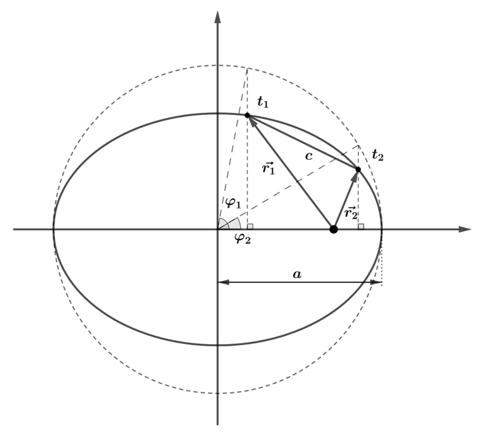
We first assume that the orbit of the object is a circular orbit, and an objective function can be constructed using the angular data obtained from observations [28]. Obviously, in theory Δ n ( a ) = 0 .
Δ n ( a ) = n 1 ( a ) n 2 ( a )
where
n 1 ( a ) = μ a 3 , n 2 ( a ) = arccos r 1 r 2 a 2 1 Δ t 1 + 3 J 2 4 a 2 6 8 sin 2 i .
The i is the inclination of orbit. According to Kepler’s third law, n 1 in Equation (23) can be calculated directly from the assumed a 
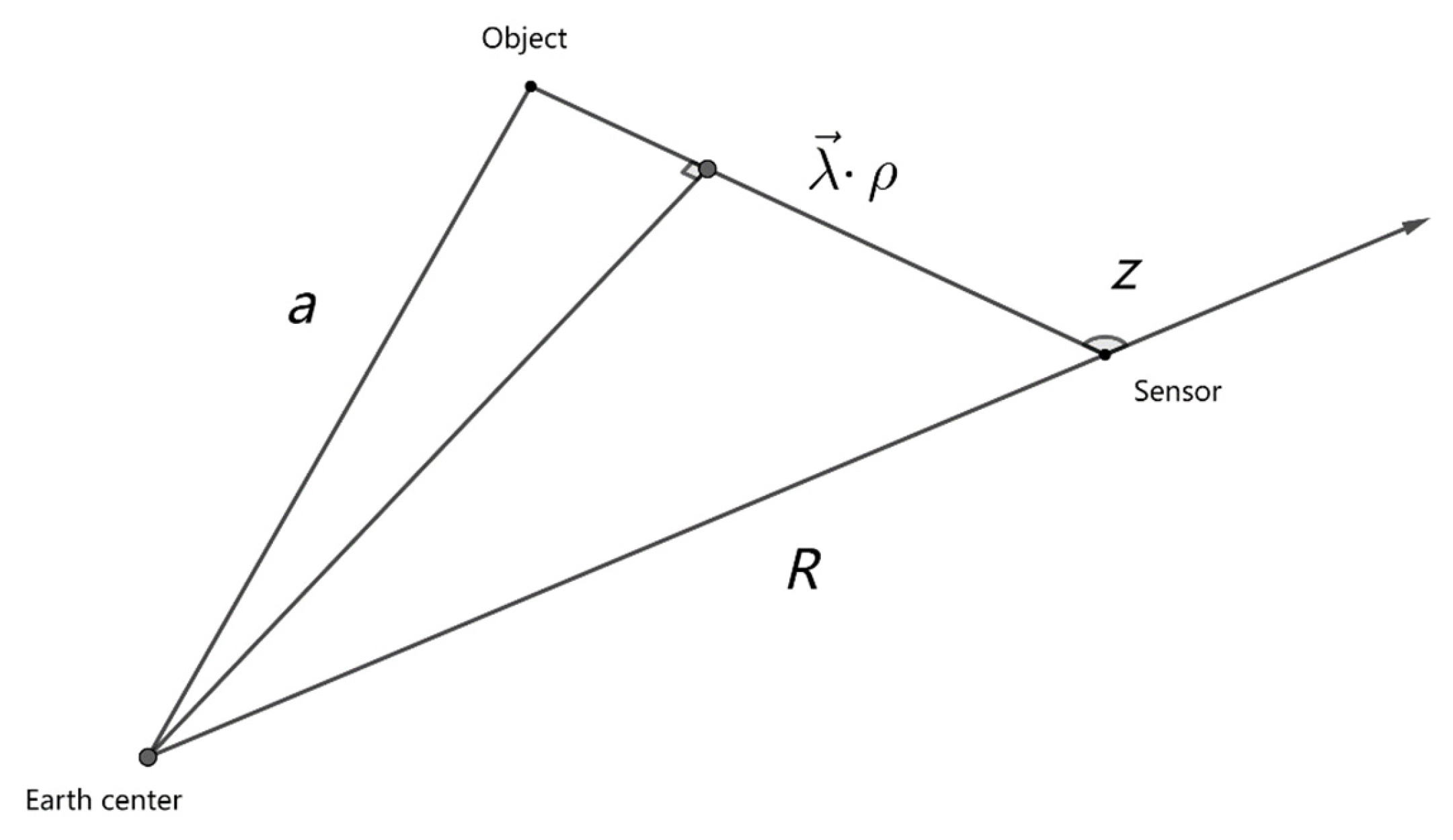
. The computation of n 2 obviously needs the geocentric vectors r 1 and r 2 of the target, which are computed as follows:
r i = ρ i λ i + R i
ρ i = a 2 R i 2 sin 2 z i R i cos z i
R i cos z i = λ i R i
R i 2 sin 2 z i = R i 2 R i cos z i 2
where z i is the zenith angle. The geometric relationships are shown in Figure 3.
Finally, fast convergence can be achieved by using Newton’s iterative method (the initial value can be chosen as a = 10 , 000 km ). Thus, the required initial value is obtained ( ρ 1 and ρ 2 ).
Since the above process is performed under the assumption that the orbit is circular, further processing is required to minimize the effect of eccentricity. From Equations (6)–(9), it can be seen that when the angle between the geocentric vectors of the two calendar elements is fixed, the larger the modulus of the two vectors, the larger x is. From Equation (23), it can be seen that the solution of Δ n 2 involves only the angle of the vectors. So, when x is too large, it is usually caused by r 1 or r 2 being too large. The problem can be solved by reducing ρ 1 and ρ 2 . Since the eccentricity of the LEO target is generally less than 0.25 [29], the corrections ( Δ ρ 1 and Δ ρ 2 ) can be set to 10% of the values of ρ 1 and ρ 2 , and several iterations will converge.

3.2. Improvement of the Objective Function

In Section 2.2, Question (II) is posed. From Equation (12), it can be seen that there is no essential difference in the geometrical relationship between the ground-based optical surveillance and the space-based optical surveillance. Lambert’s equation is built on the basis that the object follows Kepler’s motion as follows:
r ¨ = μ r 3 r .
Clearly, the motion of ground-based sensors does not follow this equation, whereas space-based sensors do. Thus, the object position vector r j = R j when ρ i = 0 in Equation (12). For space-based platforms, this still satisfies the solution of Lambert’s equation. By substituting this result into the objective equation, it can be found that there is still a solution.
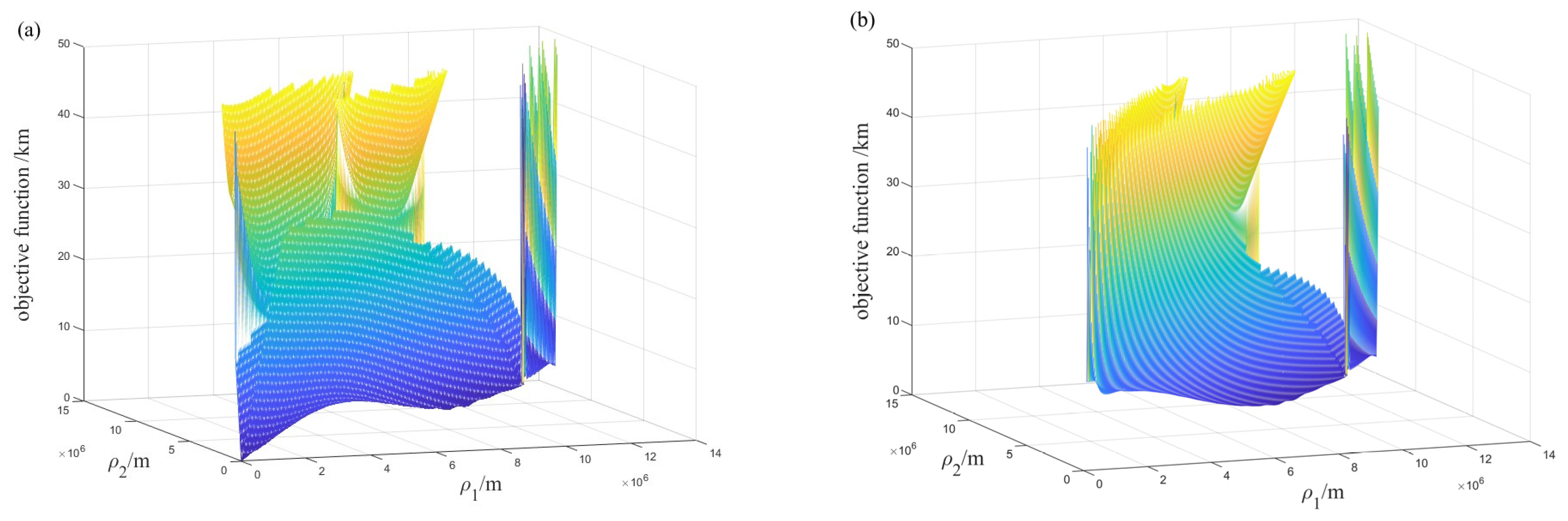
To remove this trivial solution, the objective Function (29) needs to be downgraded.
f = | ρ c | sin λ 3 , λ c .
The objective function after being downgraded is f | ρ c | = sin λ 3 , λ c = 0 . It can be noticed that the objective function becomes dimensionless. Since the magnitude of the independent variable is in units of length, if this value is used for iteration, the deviation from its required corrective value is too large. Therefore, the objective function can be set to f | ρ c | r c . Since the minimum value of r c is min { R 3 sin z 3 , R 3 } when ρ c > 0 , the objective equation constructed by this function will no longer have a trivial solution. Figure 4 illustrates two objective function figures. It can be seen that (a) is a figure of the original objective function with two equation solutions, one of which is the trivial solution, while (b) is the figure of the improved objective function; there is only one solution to the equation, and it still has the original convergence.

3.3. Restricted Corrective Value Solution Method

Gooding’s method has a high success rate but still fails to converge on about 10% of the data. This is mainly caused by the large deviation from the corrective value. When the independent variable is in the region where the slope tends to zero and the function value is again large, according to Equation (19), the corrected value becomes extremely large at this point. In the case of reasonable initial values, this is mainly due to the large corrective value, which leads to an error in the x > 1 or ρ i < 0 obtained from the independent variable. Therefore, the problem that the independent variables will iterate to unreasonable values needs to be removed. In this paper, we propose an approach to corrective value-solving using constraints.
When the independent variable appears to be less than 0 (i.e., ρ 1 + D 1 < 0 or ρ 2 + D 2 < 0 ), let D 1 n e w = D 2 n e w = 1 , 000 , 000 m i (where i is the number of times the independent variable appears to be less than 0). Similarly, for the independent variable corresponding to the desired x > 1 , let D 1 n e w = f s i g n ( D 1 ) D 1 , D 2 n e w = f s i g n ( D 2 ) D 2 , where f s i g n is a signum function, −1 when the parameter value is greater than 0, and 1 otherwise.

3.4. Fitted-Curve Noise Suppression Method

In a certain observation condition for many repeated measurements or in a time series of measurements, there is always a value and sign are not fixed, without any law of change, but the overall compliance with certain statistical characteristics (mean, variance and distribution) of the error is called random noise. Problem (IV), obtained from the analysis, shows that this error has a non-negligible effect on the Gooding method.
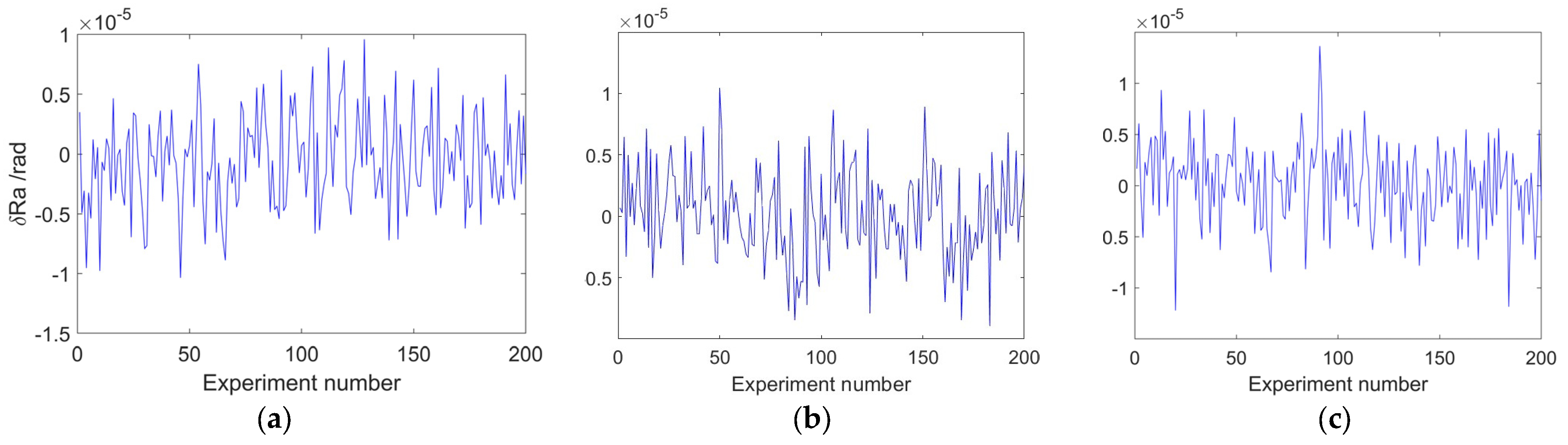
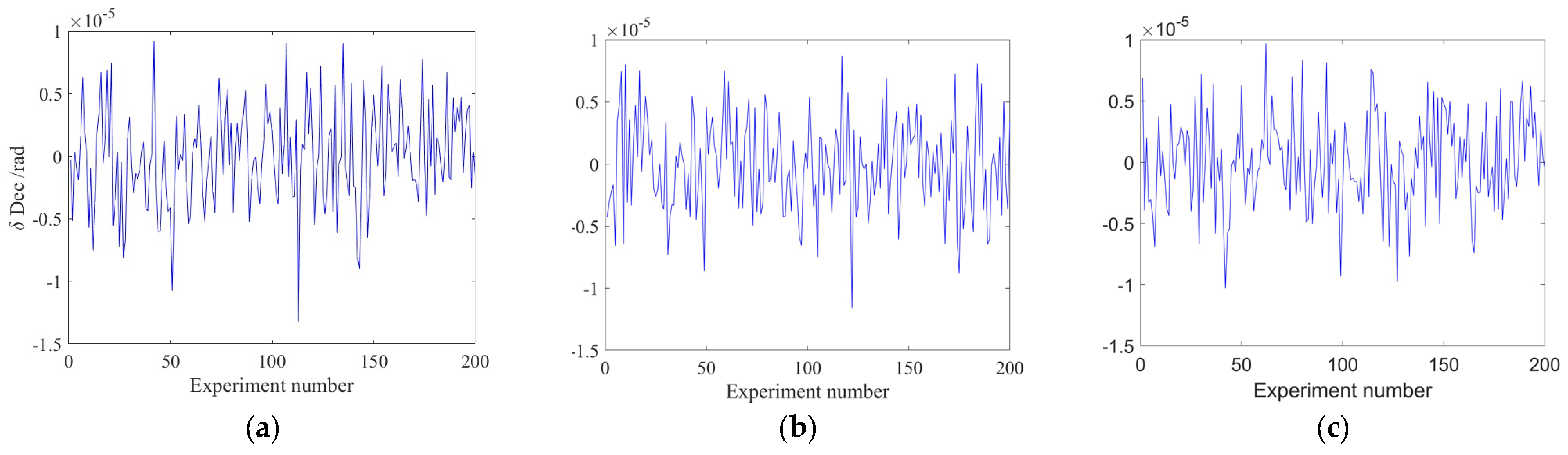
Polynomial fitting is simple, fast, and practical, which is more suitable for quickly solving the initial orbit. Two important parameters that affect the effectiveness of polynomial fitting are the number of fitted points and the polynomial order. Since the observational arc segment is very short, the variations in both right ascension and declination are extremely small, and the change process is smooth. Therefore, the improvement needs can be achieved by using a third–order polynomial and fitting using all observations. For validation, the existing observations are added to 4″ Gaussian noise and then processed and compared with higher–order polynomial fitted-curve noise suppression, respectively, and the results are shown in Figure 5 and Figure 6.
The three respective plots in Figure 5 and Figure 6 show, from left to right, the error compared to the original observation after noise suppression of the data points using third–, fifth–, and seventh–order polynomials. It can be seen that the processed error is on the order of 10−6, with an RMS value of about 3.8 × 10⁻⁶. This shows that the method is effective in minimizing the original noise. Also, from the comparison, it can be seen that higher-order polynomials do not provide better noise suppression.
Aiming at the specific characteristics of space-based space debris observation and combining with the improvement method proposed above, this paper proposes a very-short–arc IOD method for LEO objects applicable to space–based sensors, the main flow of which is shown in Figure 7.

4. Results

4.1. Simulated Data

To validate the applicability of the proposed space-based IOD method, simulated data are designed in this paper. The SWARM B satellite is selected as a space-based sensor. The first set of data is obtained by predicting the global laser satellite observation data from the ILRS (International Laser Ranging Service, LRS, Greenbelt, MD, USA) official website (http://ilrs.gsfc.nasa.gov (accessed on 12 August 2023)) after precise orbit determination. Another set of data comes from observations from the electrical-optical telescope array (EA) at the Changchun Observatory. Observations after precise orbit determination are predicted and then converted to the space-based sensor to obtain space-based space debris observations.
NP (normal point data) is a data product provided free of charge by ILRS (International Laser Ranging Service, LRS) to researchers around the world, aiming to provide key technical support and assurance for research in the fields of geodynamics, geodesy, geophysics, and astronomy [30]. The electrical-optical telescope array (EA) at the Changchun Observatory consists of eight transmission optical telescopes, imaging detectors, telescope bases, master computers, GPS clocks, and observational positioning software systems. Each telescope has an aperture of 150 mm, a focal length of 150 mm, a field of view of 198.81 square degrees, and an overall surveillance sky coverage of up to 1590 square degrees. The main observation object size can reach a 0.5~1 m space object; the time interval of the angular data of the same object is about 1.7 s; and the error is about 8 arcseconds. In addition, each telescope has a CCD camera with a resolution of 3056 pixel × 3056 pixel and a dedicated computer for image processing [31,32,33]. Figure 8 shows a physical view of the device.
Figure 9, Figure 10 and Figure 11 show the target orbital characteristics of the two data sources, with a total of 59 NP objects and 1330 objects observed by EA.

4.2. IOD Results

Firstly, the noise suppression effect is verified. A 4″ Gaussian noise error is added to the original NP data to generate control data. The same initial values (error less than 100 km) are used, and both utilize the Gooding method for IOD, and the results are shown in Table 1. Since the position of the orbit is mainly related to SMA, inclination, and the right ascension of the ascending node, the results of the comparison of the three errors are shown in the table.
Secondly, the SIVD is tested using the same data with a 4″ Gaussian noise error. The initial orbit determination is performed by Gooding. The SIVD was used for one set of tests, and the usual initial value of 1.1 times the Earth’s radius was chosen for the other; the results are shown in Table 2. Thirdly, Table 3 demonstrates the validation of the improved objective equation using the same data. The initial value is 1.1 times the Earth’s radius. Then, the restricted corrective value solution method is also validated using the control variables method, and the result is shown in Table 4.
Finally, the validation of the improved method is carried out using larger quantities of simulated data obtained from EA and real-world ground-based observations from EA. The initial orbit is determined using the Gooding method and the proposed method for the above-simulated data. The data arc length is 30 s to 40 s. In this paper, the success of IOD is defined as the size of its SMA, ranging from 6400 km to 20,000 km in the case that the iterative solution can converge. Since the table shows that 97% of the SMA errors of the proposed method are less than 200 km, this definition does not make the results favorable to one side of the proposed method. For simulated data obtained from EA, Table 5 shows the statistical results of the SMA errors computed by the two methods, as well as the success rates. Table 6 demonstrates the error statistics for the inclination and the right ascension of the ascending node.
For real-world ground-based observations from EA, Table 7 shows the results of processing using the Gooding method, the improved Gooding (I-Gooding) [26], the RS method (range-search-based IOD method, RS method) [20], and the proposed method. The I-Gooding method is to change the matrix of iteration coefficients (calculated from the observed data with errors) by using the matrix of iterative coefficients obtained from multiple observations to improve the iterative process. The error O C of the result can be found by obtaining all the orbital parameters obtained from Two Line Elements (TLEs) of the public NORAD (North American Aerospace Defense Command, NORAD, Colorado Springs, CO, USA) catalog. Due to the cyclic variation of the right ascension of the ascending node, the statistics of its error extend to 3°. Also, the average computation time for each algorithm was counted. The above experiments are implemented on the MATLAB R2022a platform based on the MATLAB language. The processor of the computer used for the experiment is an AMD Ryzen 5 5600U with Radeon Graphics 2.30 GHz.

5. Discussion

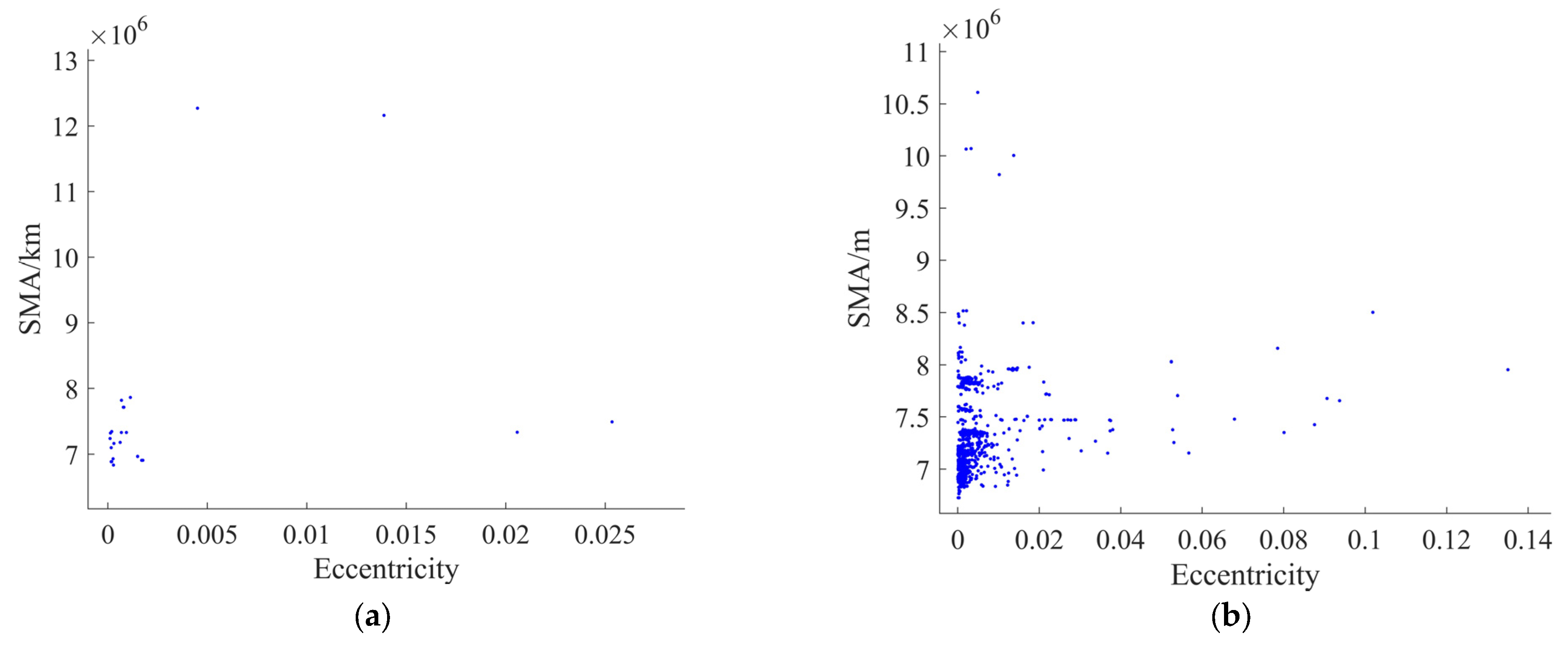
The simulated data are reasonable. From Figure 9, we can see that the objects’ SMA (semi-major axis) ranges from 6500 km to 13,000 km, and the eccentricity ranges from 0 to 0.14. In addition, the eccentricity of less than 0.05 and the SMA of less than 8500 km are both 99% of the quantity. From 
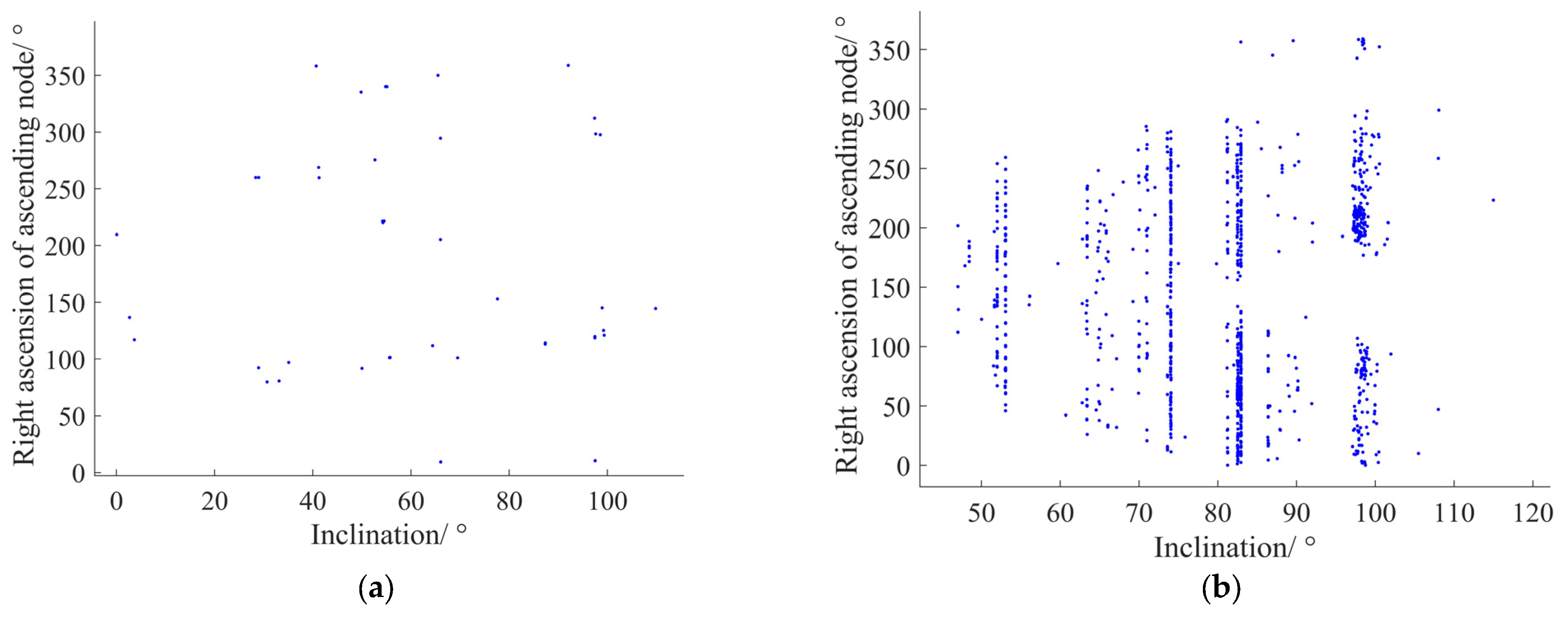
Figure 10, it can be seen that the objects’ inclination ranges from 0 to 360°, and the right ascension of the ascending node ranges from 0 to 120° (this has a strong relationship with the sensor’s location at high latitudes and its observation methodology). However, Figure 10b shows that some objects have the same inclination. Many of these co-planar satellites are star-link satellites. 
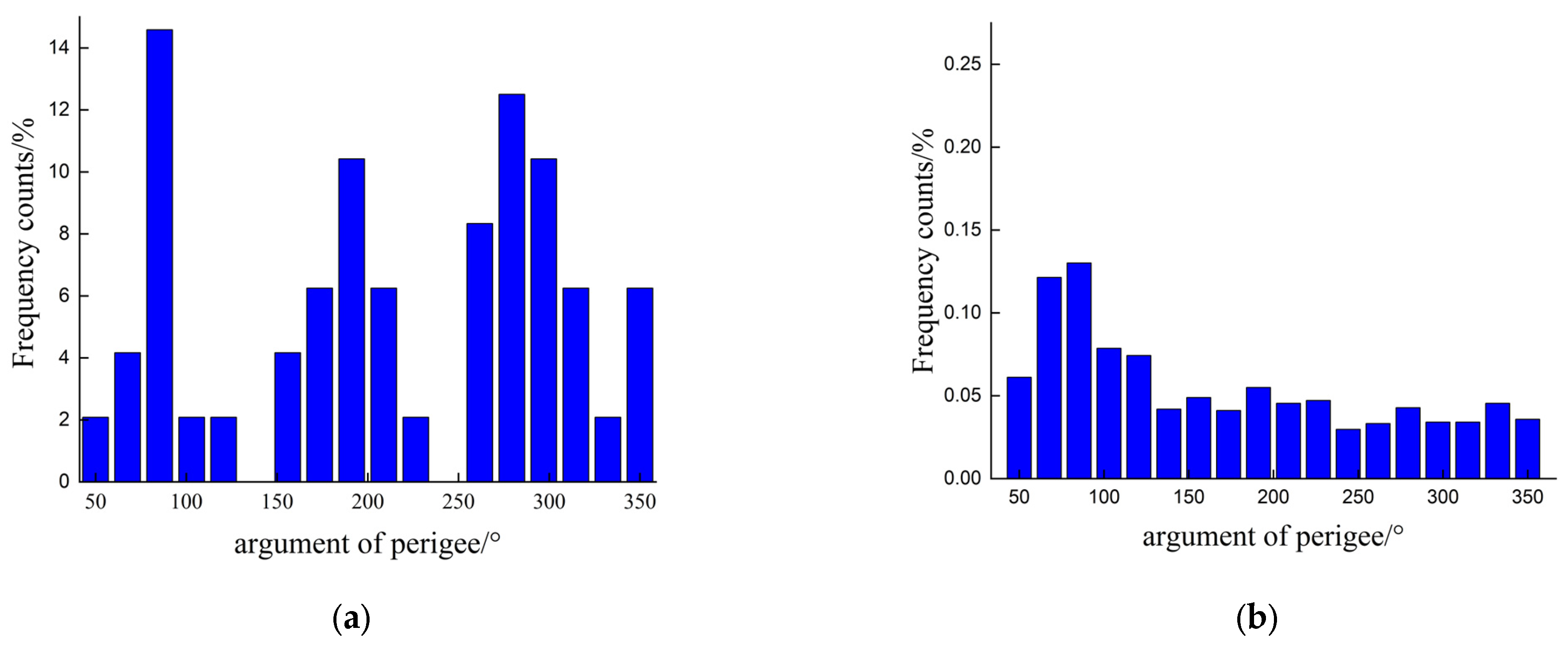
Figure 11 shows that the argument of perigee ranges from 0 to 360°. As can be seen, these data distributions above are comprehensive and homogeneous and contain the orbital characteristics expected of LEO targets.
From Table 1, it can be seen that after processing with the proposed noise suppression method, the accuracy of each track is significantly improved. The improvement in the SMA, the inclination, and the ascending node declination is relatively greater, reaching 32%, 40%, and 47.5%, respectively. At the same time, this shows that the 4″ level of noise error in the observations does have a significant influence on the IOD calculation using the Gooding method. However, in conjunction with Figure 5 and Figure 6, it can be seen that the processed observations still have Gaussian noise errors of about 1″ and still affect the IOD results. Therefore, the proposed method may not give better results when the accuracy of the observation equipment used is high.
The SIVD method and the improvement of the objective function have significantly improved the accuracy of the Gooding method for processing space-based observations. From Table 2, it can be seen that the Gooding method with SIVD has better performance for solving each parameter. The improvement reaches 40~65%. This is mainly due to the fact that the SIVD can provide an initial value with a small error, which makes the convergence result converge to the true solution instead of incorrect solutions (e.g., trivial solutions, negative values, etc.) and also reduces the number of iterations. The result shown in Table 3 indicates that the improved objective function allows the Gooding method to be applied to space-based observations. In the example of the SMA, the percentage of errors less than 200 km reaches 83%, which is a 33% improvement compared to the Gooding method. The improved objective equation removes the trivial solution, which makes it possible for even large errors in the initial value not to cause the result to converge to the trivial solution, so the overall accuracy is improved. From Table 4, we can see that the restricted corrective value solution method offers relatively little improvement to the Gooding method, mainly due to the fact that the corrective value does not have a significant effect on the solution and convergence trend.
The improved method in this paper has better performance in processing larger quantities of simulated space-based data. As can be seen from Table 5, the method proposed in this article has better performance in terms of success rate, reaching 99%. Secondly, for each interval of the semi-major axis error, the proposed method is consistently better than the Gooding method. Especially in the smaller error interval of ≤20 km, the proposed method accounts for 71%, equivalent to 2.4 times that of the Gooding method. In Table 6, it can be seen that the proposed method still performs better. Within the error range of ≤1°, the proportions of the proposed method’s output results are 2 to 3 times higher compared to the Gooding method and are all above 90%. Then, the proposed method still performs better in intervals where the error is much smaller. Taking the error of the right ascension of the ascending node as an example, within the error range of ≤1°, the proportion of the proposed method’s output results is 3.1 times higher compared to Gooding’s method, reaching 49%. Next, the comparison reveals that the algorithms in this paper have the same and uniform degree of accuracy enhancement for the inclination and the right ascension of the ascending node.
The improved method has the best performance in processing larger quantities of real-world data (results in Table 7). Firstly, in terms of success rate, the proposed method still achieves a success rate of 99%, which shows that it has excellent stability in handling different types of data. Secondly, the proposed method inherits the computational efficiency of the Gooding method, and due to the characteristics of the geometric model used in the method, the computational speed of the method does not decrease due to the increase in the number of data points in the arc length. The computing time of the average improvement method is about 0.07 s, which is much less than the period (1~2 s) for the sensor to collect data. The I-Gooding method has a 61% success rate. This is mainly due to the fact that the method requires an initial value with high precision (error less than 5 km), and the experience threshold also affects the result [26]. The average computation times of the RS method and the I-Gooding method are 0.82 s and 0.38 s, respectively. This is because both of them need to compute all the observations of a segment (the computation time increases as the arc length increases), and the RS method needs to perform the orbital prediction, so its computation time is longer.
In terms of accuracy, the proposed method performs best on all three orbit parameters of the solutions. Three methods have the same performance in terms of inclination errors. The Gooding method has a significant gap in solving SMA relative to the other two methods. Errors of less than 3° in the right ascension of the ascending node reached only 89% of the solutions calculated by the RS method. This may be related to its general performance in describing track-plane pointing [26].
Through the above experimental results, it can be seen that the proposed method is better than the Gooding method in terms of overall results. First, the proposed methods all achieved a success rate of about 99%. Secondly, in terms of error, there is an improvement in all orbital parameters. For example, in terms of the SMA of the orbit, the proportion of results with an error of less than 100 km is around 94%. Compared to the Gooding method, this result has improved by nearly double. The proposed method also performs well in terms of computational efficiency. The average computation time is about 0.065 s, which is much smaller than the arc length of the observed data as well as the sampling period.

6. Conclusions

In this paper, the Gooding method is analyzed for application to IOD in space-based observation environments, and a new method for IOD is proposed based on it. We evaluate the proposed method in comparison to the Gooding method, and the simulation results not only validate our theoretical derivation but also show that the overall results of the proposed method are better than those of the Gooding method. Among them, the proposed method can reach 99% in terms of success rate. The proportion of computed results with an SMA error of less than 100 km, an inclination error of less than 1°, and a right ascension of the ascending node of less than 1° all exceed 90%. Since IOD is the key to cataloging space debris, the proposed method would significantly contribute to cataloging space debris in the future. For example, the higher the initial orbit accuracy, the faster the convergence speed of accurate orbit determination. In addition, with higher accuracy of the initial orbit parameters, the arc segments can be briefly categorized, which is very helpful for the efficiency of the initial orbit association. Secondly, the improvement of its success rate is also based on this. In the future, we plan to conduct a study of the initial orbit association based on the proposed method, followed by applying the method to the IOD of GEO objects and analyzing its performance. Meanwhile, we will further study the noise processing of the observations in the hope of finding a more effective noise-suppression method.

Author Contributions

Writing, Y.Y. and Z.L.; resources, Y.Y.; data curation, Y.Y., Z.L., C.L. and J.S.; funding acquisition, Z.L. and Z.K.; writing—review and editing, L.C. All authors have read and agreed to the published version of the manuscript.

Funding

This research is funded by the National Natural Science Foundation of China (NSFC) (grant number 12273080) and the Joint Research Fund in Astronomy (U2031129) under cooperative agreement between the National Natural Science Foundation of China (NSFC) and Chinese Academy of Sciences (CAS).

Data Availability Statement

Not applicable.

Acknowledgments

The authors would like to gratefully acknowledge the financial support kindly provided by the National Natural Science Foundation of China (NSFC) (grant number 12273080) and the Joint Research Fund in Astronomy (U2031129) under cooperative agreement between the National Natural Science Foundation of China (NSFC) and Chinese Academy of Sciences (CAS).

Conflicts of Interest

The authors declare no conflict of interest.

References

  1. Qiao, K.; Wang, Z.; Cong, M. Analysis on space based and ground based surveillance system to space target. Opt. Tech. 2006, 32, 744–749. [Google Scholar]
  2. Yu, J.; Su, Z.; Tan, Q. Analysis on the space-based optic observation mode for space object. Chin. J. Quantum Electron. 2006, 23, 772–776. [Google Scholar] [CrossRef]
  3. Li, B.; Sang, J.; Chen, J. Achievable orbit determination and prediction accuracy using short-arc space-based observations of space debris. Adv. Space Res. 2018, 62, 3065–3077. [Google Scholar] [CrossRef]
  4. Kennewell, J.A.; Vo, B.N. An overview of space situational awareness. In Proceedings of the 16th International Conference on Information Fusion, Istanbul, Turkey, 9–12 July 2013; pp. 1029–1036. [Google Scholar]
  5. Zhao, G.; Liu, L.; Li, B.; Li, Z.; Sang, J. An orbit determination approach to associating optical tracklets of space objects. Acta Astronaut. 2022, 200, 506–523. [Google Scholar] [CrossRef]
  6. Vallado, D.A. Fundamentals of Astrodynamics and Applications, 4th ed.; Microcosm Press: Hawthrone, CA, USA, 2013; pp. 433–443. [Google Scholar]
  7. Schaeperkoetter, A. A Comprehensive Comparison between Angles-Only Initial Orbit Determination Techniques. Master’s Thesis, Texas A & M University, College Station, TX, USA, December 2011. Available online: https://hdl.handle.net/1969.1/ETD-TAMU-2011-12-10242 (accessed on 14 August 2023).
  8. Chen, L.; Liu, C.; Li, Z.; Sun, J.; Kang, Z.; Deng, S. Non-Cooperative Common-View Observation of LEO Space Objects and Initial Orbit Determination. Acta Opt. Sin. 2021, 41, 6. [Google Scholar] [CrossRef]
  9. Lei, X.; Li, Z.; Du, J.; Chen, J.; Sang, J.; Liu, C. Identification of uncatalogued LEO space objects by a ground-based EO array. Adv. Space Res. 2021, 67, 350–359. [Google Scholar] [CrossRef]
  10. Jia, P.; Wu, L.A. Robust algorithm of the initial orbit determination. Acta Astron. Sin. 2000, 41, 123–128. [Google Scholar] [CrossRef]
  11. Wang, X. A Robust Method of Preliminary Orbit Determination. Acta Astron. Sin. 2013, 37, 274–281. [Google Scholar] [CrossRef]
  12. Lu, B.K.; Rong, P.Z.; Wu, J.M. The unit vector method for initial orbit determination of artificial satellite. J. Astronaut. 1997, 18, 7–14. [Google Scholar]
  13. Liu, L.; Xi, X.; Chen, H. An Initial Orbit Determination Method Using Space-based Angle Data. J. Natl. Univ. Def. Technol. 2009, 49, 11–15. [Google Scholar] [CrossRef]
  14. Gan, Q.; Ma, J.; Lu, B. An Initial Orbit Determination Method Using Inter Satellite Angle Measurement. J. Astronaut. 2007, 28, 619–622. [Google Scholar]
  15. Der, G.J. New angles-only algorithms for initial orbit determination. In Proceedings of the Advanced Maui Optical and Space Surveillance Technologies Conference, Maui, HI, USA, 11–14 September 2012. [Google Scholar]
  16. Milani, A.; Gronchi, G.F.; Knežević, Z.; Sansaturio, M.E.; Arratia, O. Orbit determination with very short arcs: II. Identifications. Icarus 2005, 179, 350–374. [Google Scholar] [CrossRef]
  17. Zhao, G. Orbit Determination by Fitting Probability Distribution on Space Object Admissible Region Using Gaussian Mixed Model. Ph.D. Thesis, School of Geodesy and Geomatics, Wuhan University, Wuhan, China, May 2020. [Google Scholar]
  18. DeMars, K.J.; Jah, M.K. Probabilistic initial orbit determination using gaussian mixture models. J. Guid. Control Dyn. 2013, 36, 1324–1335. [Google Scholar] [CrossRef]
  19. Huang, J.; Lei, X.; Zhao, G.; Liu, L.; Li, Z.; Luo, H.; Sang, J. Short-Arc Association and Orbit Determination for New GEO Objects with Space-Based Optical Surveillance. Aerospace 2021, 8, 298. [Google Scholar] [CrossRef]
  20. Sang, J.; Lei, X.; Zhang, P.; Pan, T.; Li, H. Orbital solutions to LEO-to-LEO angles-only very short-arc tracks. In Proceedings of the 7th European Conference on Space Debris, Darmstadt, Germany, 18–21 April 2017. [Google Scholar]
  21. Blanchard, R.C.; Lancaster, E.R. A Unified Form of Lambert’s Theorem; National Aeronautics and Space Administration Publishing: Greenbelt, MD, USA, 1969; pp. 1–13. [Google Scholar]
  22. Gooding, R.H. A New Procedure for Orbit Determination Based on Three Lines of Sight (Angles Only); Farnborough Publishing: Hampshire, UK, 1993. [Google Scholar]
  23. Gooding, R.H. A procedure for the solution of Lambert’s orbital boundary-value problem. Celest. Mech. Dyn. Astron. 1990, 48, 145–165. [Google Scholar] [CrossRef]
  24. Ansalone, L.; Curti, F. A genetic algorithm for initial orbit determination from a too short arc optical observation. Adv. Space Res. 2013, 52, 477–489. [Google Scholar] [CrossRef]
  25. Li, X.; Wang, X. Particle Swarm Optimization for Initial Orbit Determination with Too-Short-Arc. J. Spacecr. TTC Technol. 2015, 34, 545–551. [Google Scholar]
  26. Zhang, Z. Improving Gooding Initial Orbit Determination Method. Master’s Thesis, School of Geodesy and Geomatics, Wuhan University, Wuhan, China, April 2021. [Google Scholar]
  27. Gooding, R.H. On the Solution of Lambert’s Orbital Boundary-Value Problem; Royal Aerospace Establishment Publishing: Farnborough Hants, UK, 1988; pp. 1–49. [Google Scholar]
  28. Wu, L.; Xiong, J.; Niu, Z.; Xiao, W. Space-Based Detection of Space Target; China Science Publishing: Beijing, China, 2017. (In Chinese) [Google Scholar]
  29. Bulk Download Alternative. Available online: https://www.space-track.org/#recent (accessed on 14 August 2023).
  30. An, N.; Guan, B.; Zhang, Y.; Gao, J.; Wen, G.; Dong, X.; Ma, L.; Fan, C. Development review of satellite laser ranging data processing technology. Infrared Laser Eng. 2021, 50, 206–214. [Google Scholar] [CrossRef]
  31. Ding, Y. Observation Data Analysis of Space Objects with Space Debris Photo-Electric Telescope Array. Master’s Thesis, University of Chinese Academy of Sciences, Changchun, China, June 2019. [Google Scholar]
  32. Li, Z. Research in Optoelectronic Observation Technologies for Space Objects. Ph.D. Thesis, University of Chinese Academy of Sciences, Changchun, China, May 2014. [Google Scholar]
  33. Changchun Observatory of National Astronomical Observatory, Chinese Academy of Sciences. Array Structured Space Debris Photoelectric Observation System: CNl04570319[A].2015-4-29; Changchun Observatory of National Astronomical Observatory, Chinese Academy of Sciences: Changchun, China, 2015. [Google Scholar]
Figure 1. Figure of Lambert’s equation construction.
Remotesensing 15 05217 g001
Figure 2. Schematic figure of objective function construction.
Remotesensing 15 05217 g002
Figure 3. Geometry to compute geocentric vectors.
Remotesensing 15 05217 g003
Figure 4. Objective function. (a) Figure of the original objective function; (b) Figure of improved objective function. (The above figures are obtained by thresholding the function values, which are retained when the function value is less than 50,000 m and set to null when it is greater than that.).
Remotesensing 15 05217 g004
Figure 5. Right ascension error after the fitted-curve noise suppression method with different polynomial orders. (a) third–order polynomial; (b) fifth–order polynomial; (c) seventh–order polynomial.
Remotesensing 15 05217 g005
Figure 6. Declination error after the fitted–curve noise suppression method with different polynomial orders. (a) third–order polynomial; (b) fifth–order polynomial; (c) seventh–order polynomial.
Remotesensing 15 05217 g006
Figure 7. Flowchart of the improved Gooding method.
Remotesensing 15 05217 g007
Figure 8. The electrical-optical telescope array (EA) at the Changchun Observatory.
Remotesensing 15 05217 g008
Figure 9. Distribution of SMA and the eccentricity for simulated data. (a) NP; (b) observations by EA.
Remotesensing 15 05217 g009
Figure 10. Distribution of the inclination and the right ascension of the ascending node for simulated data. (a) NP; (b) observations by EA.
Remotesensing 15 05217 g010
Figure 11. Distribution of the argument of perigee for simulated data. (a) NP; (b) observations by EA.
Remotesensing 15 05217 g011
Table 1. Orbital parameter errors with and without noise suppression.
Noise SuppressionSMA ErrorsIncl ErrorsOmega Errors
<200 km<1°<1°
N50%60%40%
Y66%84%59%
Table 2. Orbital parameter errors with and without SIVD.
SIVDSMA ErrorsIncl ErrorsOmega Errors
<200 km<1°<1°
N50%43%19%
Y80%65%44%
Table 3. Orbital parameter errors with and without improved objective function.
Improved EquationSMA ErrorsIncl ErrorsOmega Errors
<200 km<1°<1°
N50%43%19%
Y83%83%57%
Table 4. Orbital parameter errors with and without the restricted corrective value solution method.
Improved EquationSMA ErrorsIncl ErrorsOmega Errors
<200 km<1°<1°
N50%43%19%
Y60%58%23%
Table 5. Performance of success rate and SMA errors of processing simulated data from EA with two IOD methods.
MethodSMA ErrorsSuccess Rate
≤20 km≤50 km≤100 km≤200 km
Gooding29%43%48%57%90%
Proposed method71%88%94%97%99%
Table 6. Performance of inclination errors and right ascension of ascending nod errors of processing simulated data from EA with two IOD methods.
MethodIncl ErrorsOmega Errors
≤0.1°≤1°≤0.3°≤1°
Gooding29%49%15%33%
Proposed method59%98%49%94%
Table 7. Performance of processing real-world ground-based observations from EA with some IOD methods.
Success RateComputing Time/sSMA Errors ≤100 kmOmega Errors ≤3°Incl Errors
≤1°
Gooding90%0.0428%98%98%
I-Gooding61%0.3834%30%35%
RS method85%0.8292%89%99%
Proposed method99%0.0793%99%99%
Disclaimer/Publisher’s Note: The statements, opinions and data contained in all publications are solely those of the individual author(s) and contributor(s) and not of MDPI and/or the editor(s). MDPI and/or the editor(s) disclaim responsibility for any injury to people or property resulting from any ideas, methods, instructions or products referred to in the content.

