An Efficient Pose Estimation Algorithm for Non-Cooperative Space Objects Based on Dual-Channel Transformer

Abstract

Non-cooperative space object pose estimation is a key technique for spatial on-orbit servicing, where pose estimation algorithms based on low-quality, low-power monocular sensors provide a practical solution for spaceborne applications. The current pose estimation methods for non-cooperative space objects using monocular vision generally consist of three stages: object detection, landmark regression, and perspective-n-point (PnP) solver. However, there are drawbacks, such as low detection efficiency and the need for prior knowledge. To solve the above problems, an end-to-end non-cooperative space object pose estimation learning algorithm based on dual-channel transformer is proposed, a feature extraction backbone network based on EfficientNet is established, and two pose estimation subnetworks based on transformer are also established. A quaternion SoftMax-like activation function is designed to improve the precision of orientation error estimating. The method only uses RGB images, eliminating the need for a CAD model of the satellite, and simplifying the detection process by using an end-to-end network to directly detect satellite pose information. Experiments are carried out on the SPEED dataset provided by the European Space Agency (ESA). The results show that the proposed algorithm can successfully predict the satellite pose information and effectively decouple the spatial translation information and orientation information, which significantly improves the recognition efficiency compared with other methods.

1. Introduction

Non-cooperative space object pose estimation is an urgent problem to be solved in the space field; it has very important application value in relative navigation, rendezvous and docking, active debris removal (ADR) on-orbit servicing (OOS), etc. [1,2,3,4,5,6]. For the special environment of on-orbit work, the pose estimation [7,8] algorithm based on a low-quality, low-power monocular sensor provides a feasible scheme for space application, and it has received extensive attention from scientific research institutions and researchers. 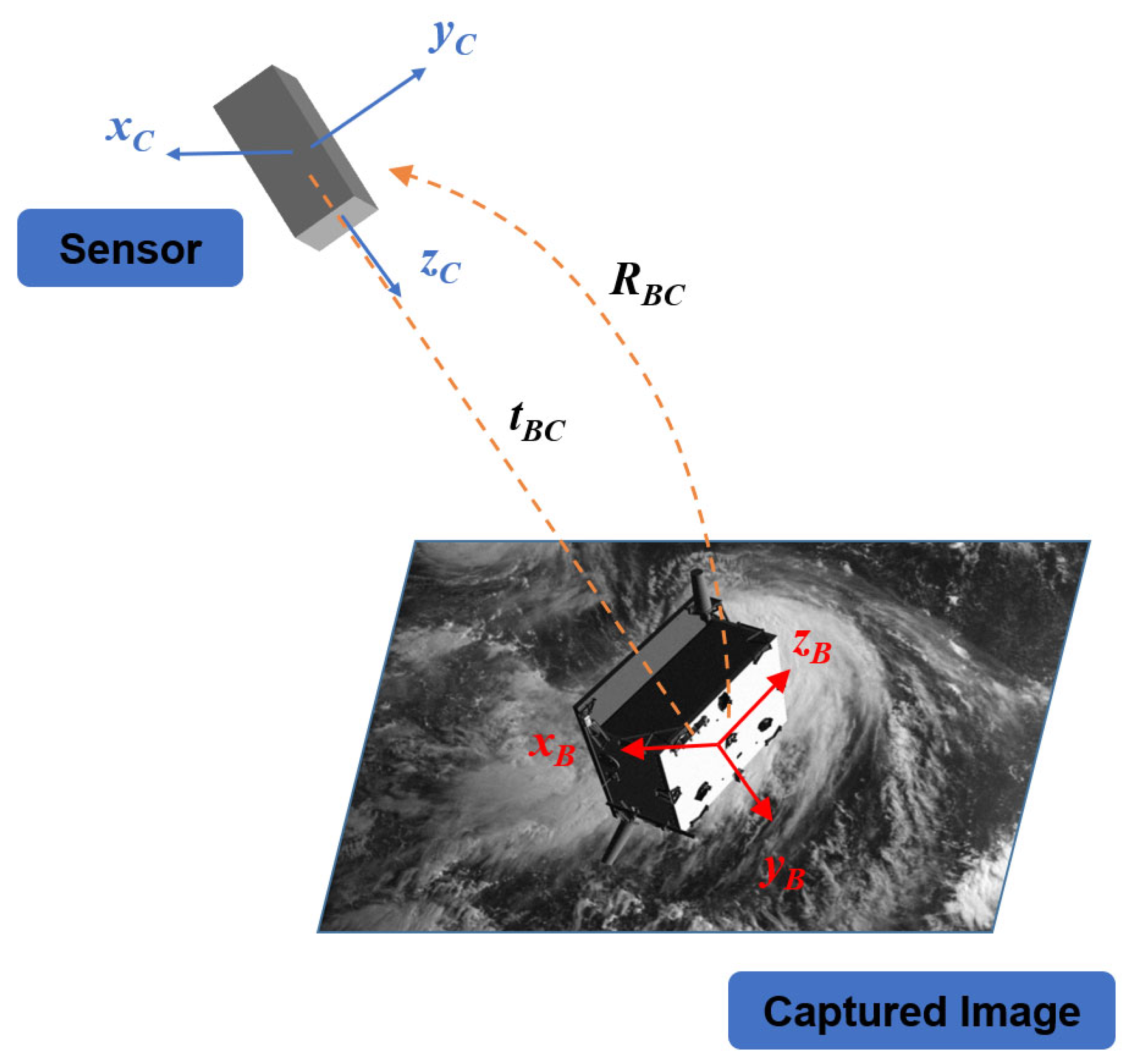Some institutions [9,10,11,12] have carried out relevant studies and semi-physical simulation experiments on the pose estimation of non-cooperative space objects by using monocular vision cameras. Compared with monocular sensors, light detection and ranging (LIDAR) and depth cameras have a smaller scope, larger size, and higher power consumption, and they are more constrained by complex space environments. Therefore, the data obtained using the monocular sensor are more consistent with the pose estimation of the non-cooperative space objects. ESA and Stanford University held the Satellite Pose Estimation Challenge competition in 2019 (SPEC2019), using a monocular sensor to photograph scale models like the Tango satellite to create the Spacecraft Pose Estimation Dataset (SPEED) [13], which was collected through semi-physical simulation experiments and the simulated space environment. The results indicate a new direction for non-cooperative space object pose estimation based on monocular vision. The positional relationship between the sensor and the satellite to be measured is shown in Figure 1.

Considering the specific mission scenario, the task of pose determination poses theoretical and technical challenges. It necessitates the discovery of optimal algorithmic solutions and sensor architectures. For non-cooperative space object pose estimation, common measurement methods include monocular sensors [14], binocular cameras [15], time-of-flight (TOF) cameras [16], LIDAR [17] sensors, laser range sensors [18], etc. Different sensors can be chosen based on the type of object, spatial environment, and satellite performance. Due to varying data output from different sensors, different processing methods can be employed. Considering factors such as on-board environment and cost, a low-power, lightweight, and cost-effective monocular sensor is more suitable. Similarly, monocular sensors are used in other pose estimation tasks, such as 2D hand pose estimation [19], camera pose estimation [20], head pose estimation [21], etc.

Over the past few decades, vision-based non-cooperative space object pose estimation has relied on manually designed features [2,22,23] that are described using feature descriptors and detected using feature detectors. These features are then detected in a 2D image, and their corresponding 3D counterparts are used to determine the relative attitude. These features include keypoints, corners, edges, etc. However, feature-based methods have defects in their generalization ability, robustness, and identification efficiency when ranging from the complex spatial environment to tens of thousands of non-cooperative space object species. With the rapid development of computing power and algorithms, the use of deep learning technology to extract features from tremendous data has been gradually applied to the field of non-cooperative space objects detection, and its powerful feature extraction as well as generalization ability can effectively solve the disadvantages of traditional methods.

Deep learning is widely used in satellite pose estimation [24,25], and it can be divided into a direct method and an indirect method. The direct method of estimating satellite pose information directly through the model has the advantages of simple process and fast estimating speed. The indirect method, however, is to deduce satellite pose information through multi-process and multi-task means. It is widely used to promote estimating precision and clarify processes. Its general processing flow [26] is as follows:

• Satellite localization network (SLN): Using object detection networks to train satellite object detectors in order to achieve precise satellite localization results.
• Landmark regression network (LRN): Input the object detected by SLN into the landmark regression network for training.
• Pose solver: The detected satellite landmarks are solved for satellite poses using PnP solver.

The UniAdelaide team [26] used the MMDetection network for object detection, then clipped out the object area and provided it to the HRNet [27] for landmark regression, and finally used PnP solver to calculate the pose information about satellite. Reference [28] used similar methods to detect satellite landmarks, whose processing was similar to the above methods, and different deep learning models were used in satellite localization network and landmark regression network. In reference [28], the transformer model was used, but it was only used in traditional landmark regression tasks. This method indicates that the model estimating process was divided into four steps, and the total processing stage took 212.1 ms. The pose estimation of non-cooperative space objects based on key point detection can detect their pose information with high accuracy, but there are problems such as being very time-consuming, having a complicated detection process [26,28,29], etc. It requires multiple steps and models to detect relevant information and requires obvious key points of non-cooperative space objects; otherwise, it is difficult to measure the CAD model and key points.

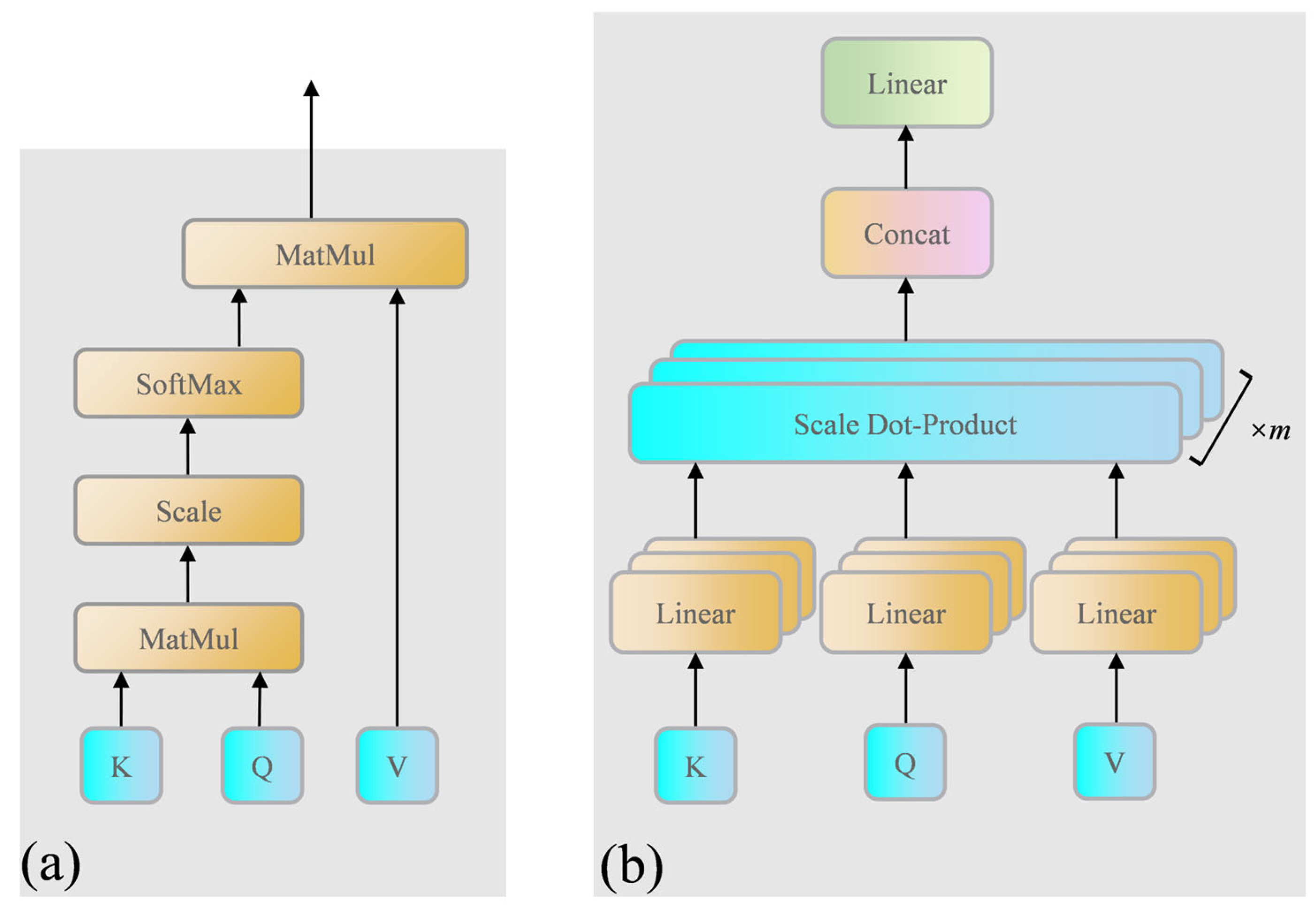
As end-to-end methods based on deep learning are widely used in industry, especially in pose estimation tasks of six degrees of freedom, deep learning models [30,31,32] based on convolutional neural networks are applied to pose estimation problems. However, convolutional neural networks have a strong feature extraction ability [33,34], but their remote modeling ability is poor, and only focusing on the feature pixels around the current pixel has limitations. Since the use of the transformer model in speech recognition in 2017, it has received extensive attention from industry and academia, and the model has achieved great success in timing information features such as natural language processing and speech recognition. Its core component, a self-attention mechanism, has powerful feature extraction and temporal correlation ability; that is, it highlights the advantages of convolutional neural network and recurrent neural network. Subsequently, transformer models led by vision transformer [35,36] and detection transformer (DETR) [37] have achieved excellent results in the field of computer vision, especially in image recognition and object detection. In reference [28], the transformer model is applied to satellite pose estimation, but this work only uses the transformer model for satellite landmark regression, whose function is consistent with the key point detection of the DETR model, and it fails to directly output the satellite pose information through an end-to-end learning structure. Combined with the advantages of the transformer model, this paper needs to explore an end-to-end pose estimation method based on the transformer model.

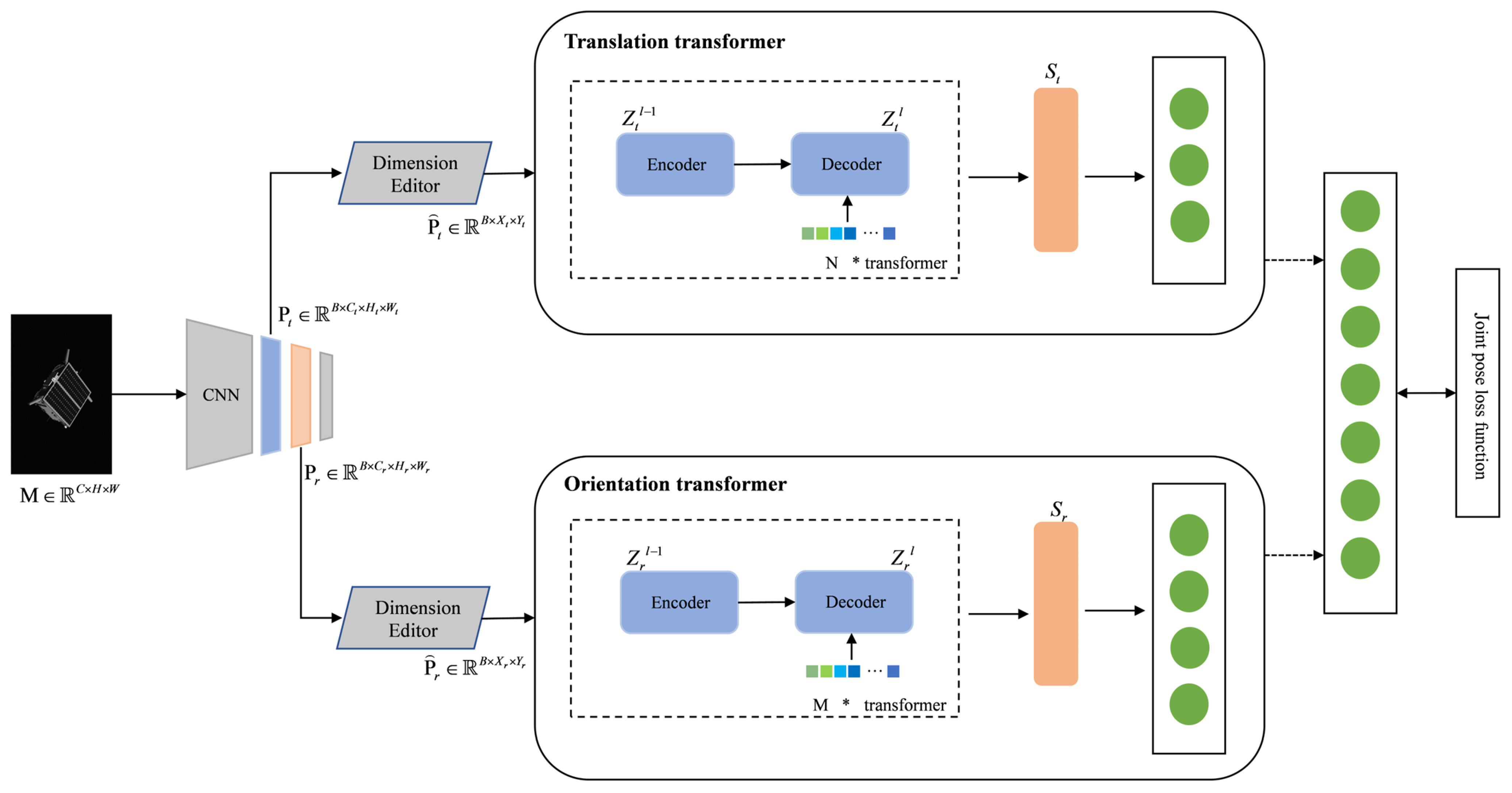
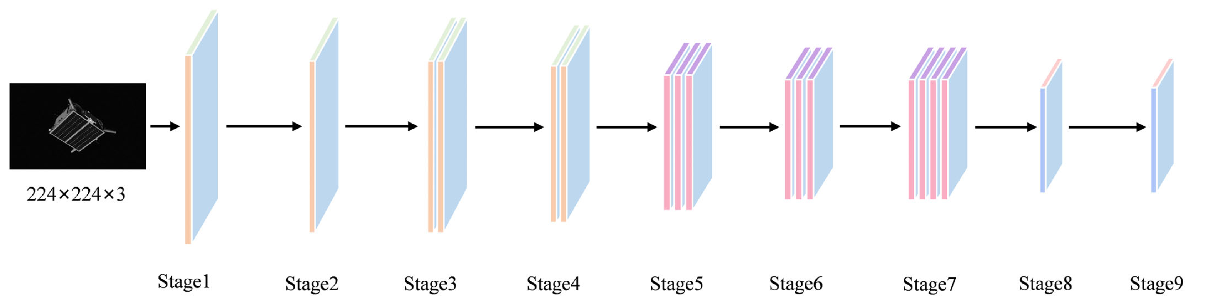
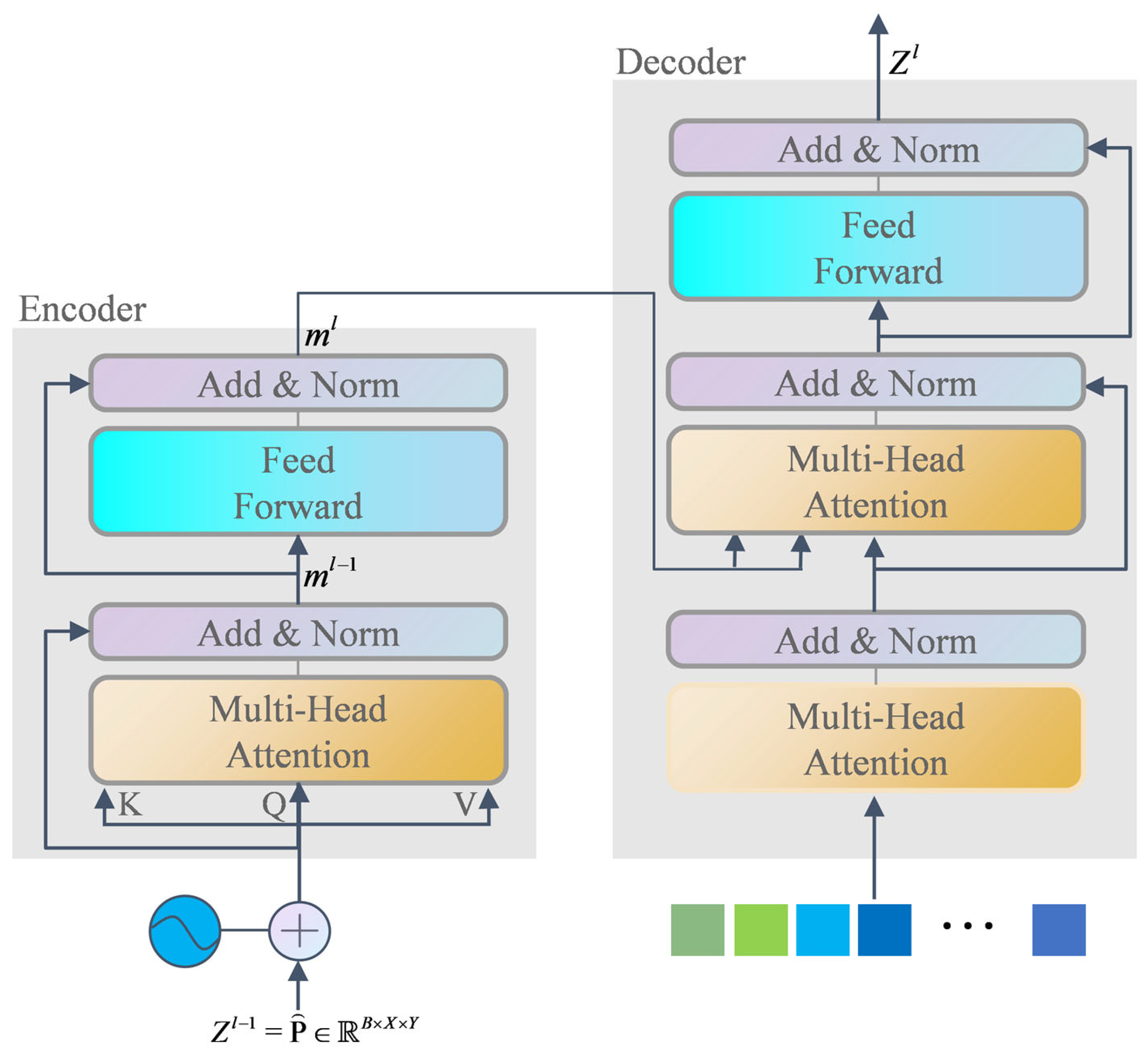
Aiming to solve the problems of the complex detection process, prior knowledge, and long detection time in existing non-cooperative space object pose estimation, this paper explores the application of the transformer model in the pose estimation of non-cooperative space objects and designs an efficient pose estimation algorithm of non-cooperative space objects based on dual-channel transformer. In this method, the pose information of non-cooperative space targets is directly output through end-to-end learning; that is, the image taken by the monocular sensor is input into the model, and the model can directly output the pose information of non-cooperative space targets without using the CAD model of the object. The algorithm uses EfficientNet as the backbone network for feature extraction and randomly selects two feature layers to input into the two pose estimation subnetworks of translation transformer and orientation transformer. The dual-channel network is used to learn translation information and orientation information, respectively, which effectively avoids the interaction between the two kinds of information. According to the characteristics of orientation information, a quaternion SoftMax-like activation function is designed to improve the accuracy of the satellite orientation information. Finally, experiments are performed on SPEED provided by ESA. The experimental results show that the proposed algorithm can successfully predict the satellite pose information, and the recognition efficiency is significantly improved compared with other methods. The main contributions of this paper are as follows:

• An end-to-end learning non-cooperative space object pose estimation network is proposed to input the images taken with a monocular sensor into the model. The model directly outputs the pose information of the non-cooperative space objects, which can simplify the estimating process of pose information.
• A dual-channel transformer non-cooperative space object pose estimation network is designed to innovatively apply transformer to the end-to-end learning satellite pose estimation task. The dual-channel network design successfully decouples the spatial translation information and orientation information of satellites.
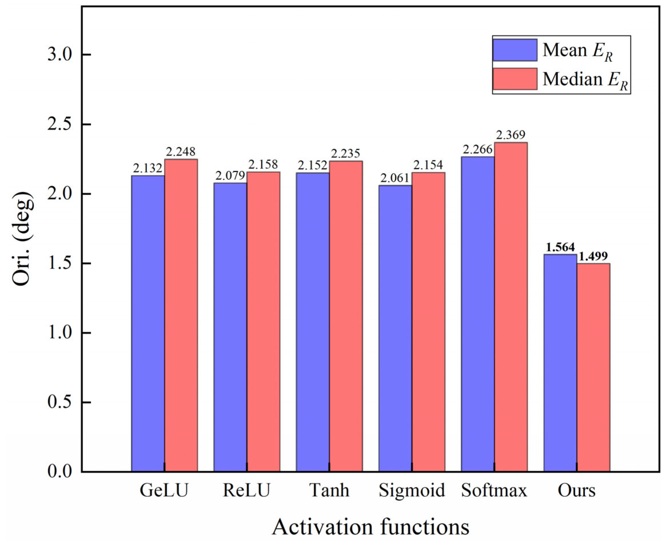
• A new quaternion SoftMax-like activation function is designed to make the model output according to the quaternion constraint so as to effectively improve the precision of orientation prediction.

The paper is structured as follows: Section 2 presents our proposed dual-channel transformer model with a quaternion activation function. We provide a detailed description of the model architecture, including the design of the dual-channel mechanism and the quaternion activation function. Section 3 focuses on the experimental setup and results analysis. First, we analyze the data used in our experiments, including their characteristics and sources. Then, we introduce the evaluation metrics employed to assess the performance of the dual-channel transformer model. Finally, we present the results of the multiple ablation experiments conducted. Furthermore, we compare the performance of our model with that of other existing models. Section 4 focuses on drawing conclusions while summarizing the innovations and beneficial effects of our work.

2. Dual-Channel Transformer Model

The dual-channel transformer model framework is shown in Figure 2. Given the satellite image $\mathrm{M}\in {\mathbb{R}}^{C\times H\times W}$, the batch size is entered as $B$. After the feature extraction network EfficientNet, two feature layers, $P_t$ and $P_r$, with different rate sizes are randomly selected and assigned to the two regression subnetworks.

In order to convert activation maps into transformer-compatible inputs, we need to convert $\mathrm{P}\in {\mathbb{R}}^{B\times C\times H\times W}$ to $\stackrel{⌢}{\mathrm{P}}\in {\mathbb{R}}^{B\times X\times Y}$. A dimension editor is designed to use 1×1 convolution to flatten the activation maps according to the processing rules, and $\mathrm{P}\in {\mathbb{R}}^{B\times C\times H\times W}$ is processed into $\stackrel{⌢}{\mathrm{P}}\in {\mathbb{R}}^{B\times X_t\times Y_t}$ and $\stackrel{⌢}{\mathrm{P}}\in {\mathbb{R}}^{B\times X_r\times Y_r}$, respectively. The transformer comprises an encoder and a decoder, and its processing flow is

$$Z^l=Decoder(Encoder(Z^{l-1})),$$

(1)

where $Z^l$ is obtained after multiple-transformer processing, and then $Z^l$ is processed as one-dimensional sequence feature $S$ through the flattening layer. We then input $S$ to the fully connected layer to output the pose information. In the orientation regression network, the quaternion SoftMax-like activation function is used.

2.1. EfficientNet Backbone Network

The relevant feature extraction backbone network is comprehensively compared, and finally the EfficientNet [38] is selected as the backbone network. The core structure is the mobile inverted bottleneck convolution (MBConv) module, which introduces the attention idea of squeeze-and-excitation network (SENet). MBConv first performs point-by-point convolution to change the dimension and then performs deep convolution, while the SE module performs point-by-point convolution to restore the original dimension after deep convolution. The model has random depth, which reduces the training time of the model. The EfficientNet structure is shown in Figure 3.

Firstly, with the feature map with the input size of 224 × 224 × 3, using 32 convolutional layers of 3 × 3 × 3 with a step size of 2 × 2, after normalization and Swish activation function processing, 112 × 112 × 32 is obtained. After preliminary processing, the features enter 16 different MBConv layers, and finally the size is 7 × 7 × 1280, and its specific network parameter is shown in

Table 1. Efficientnet-b0 network parameters.

Stage $\mathit{i}$	Operator	Resolution	Channels	Layers
1	Conv3 × 3, stride = 2	224 × 224	32	1
2	MBConv1, k3 × 3, stride = 1	112 × 112	16	1
3	MBConv6, k3 × 3, stride = 2	112 × 112	24	2
4	MBConv6, k5 × 5, stride = 2	56 × 56	40	2
5	MBConv6, k3 × 3, stride = 2	28 × 28	80	3
6	MBConv6, k5 × 5, stride = 1	14 × 14	112	3
7	MBConv6, k5 × 5, stride = 2	14 × 14	192	4
8	MBConv6, k3 × 3, stride = 1	7 × 7	320	1
9	Conv1 × 1 & Pooling & FC	7 × 7	1280	1

. In the dual-channel transformer architecture, two feature layers are randomly selected and input to the translation transformer and the orientation transformer two pose estimation subnetworks.

2.2. Transformer Model Architecture

As shown in Figure 4, the transformer consists of an encoder and decoder and consists of several network blocks. It includes positional encoding (PE), self-attention (SA), multi-head attention (MHA), feed-forward network (FFN), and residual connection and layer normalization (LN) blocks (Add & Norm), in which SA is the basic block of MHA. Transformer uses MHA to associate global features, FFN to improve model learning ability, and Add & Norm to enhance model fitting ability.

(1)

PE: The main function of the positional encoding is to retain the spatial position information between the input image blocks. The positional encoding of features is

$$\left\{\begin{array}{c}P{E}_{\left(pos,2i\right)}=\sin \left(pos/{10000}^{2i/d}\right)\\ P{E}_{\left(pos,2i+1\right)}=\cos \left(pos/{10000}^{2i/d}\right)\end{array}\right.,$$

(2)

where $PE$ is a two-dimensional matrix, the variable $\sin$ is placed in the even term of the two-dimensional matrix, and the variable $\cos$ is placed in the odd term of the two-dimensional matrix. The variable $\sin$ and the variable $\cos$ are used to form the two-dimensional matrix, and $Z^{l-1}$ is encoded in positional.

(2)

SA: Self-attention is a core component of transformer. It mimics the characteristics of biological observation targets and extracts features of some key areas by focusing attention through a mathematical mechanism. The advantages of the self-attention mechanism lie in distance learning, improved local attention, and parallel computing. As is shown in Figure 5a, the self-attention mechanism is mainly implemented using scaled dot-product attention,

$$Attention(Q,K,V)=soft\max (\frac{Q{K}^T}{\sqrt{d}})V,$$

(3)

where $Q$, $K$, and $V$ represent the query matrix, key matrix, and value matrix, respectively, which are obtained through the multiplication of feature matrix and three random weight matrices, and $d$ is the dimension of the input feature.

(3)

MHA: MHA is used to establish different projection information in multiple different projection spaces. As is shown in Figure 5b, the input matrix is projected in different ways, and the output matrix is spliced together. For each projection result, MHA executes SA in parallel;

$$hea{d}_i=Attention(Q{W}_i^Q,K{W}_i^K,V{W}_i^V),$$

(4)

where $W_i^Q,W_i^K\in {\mathbb{R}}^{d_{\mathrm{model}}\times d_k}$, $W_i^V\in {\mathbb{R}}^{d_{\mathrm{model}}\times d_v}$, and $d_{\mathrm{model}}$ represents the length of the input feature. $d_k$ = $d_v$ = $d_{\mathrm{model}}/h$, and $h$ indicates the number of heads. Concatenated the projection calculation results of multiple heads,

$$MHA(Q,K,V)=Concat(hea{d}_1,hea{d}_2,\cdots ,hea{d}_h)W^o,$$

(5)

where $W^O\in {\mathbb{R}}^{h{d}_v\times d_{\mathrm{model}}}$. Multi-head can extract the features of different heads on a more detailed level. When the total computation amount is the same as that of a single head, the feature extraction effect is better.

(4)

FFN: FFN maps features to the high-dimensional space and then to the low-dimensional space. The purpose of mapping features to the high-dimensional space is to combine the features of various types, improve the resolution ability of the model, and remove the features with low resolution through dimensionality reduction. The process is

$$FFN(x)=\max (0,W_{1}x+b_1)W_2+b_2,$$

(6)

where $W_1\in {\mathbb{R}}^{d_{\mathrm{model}}\times 4d_{\mathrm{model}}}$ and $W_2\in {\mathbb{R}}^{d_{\mathrm{model}}\times 4d_{\mathrm{model}}}$ are the learnable weights, and $b_1\in {\mathbb{R}}^{4d_{\mathrm{model}}}$ and $b_2\in {\mathbb{R}}^{4d_{\mathrm{model}}}$ are the learnable biases.

(5)

Add & Norm: Add & Norm contains residual connection and LN blocks. The residual connection can increase the processing capacity of the network depth and effectively prevent the gradient vanishing and gradient explosion. LN increases the stability of the data feature distribution and thus speeds up the convergence of the model. The formula for that is

$$F(x)=LN(m^l+m^{l-1}),$$

(7)

$$LN(x_i)=\alpha \times \frac{x_i-E(x)}{\sqrt{Var(x)+\epsilon }}+\beta ,$$

(8)

where $\alpha$ and $\beta$ are the learnable parameters and $\epsilon$ is to prevent calculation errors when the variance is 0.

2.3. Quaternion SoftMax-like Activation Function

In order to improve the expression ability of the model, activation functions are often added to the neurons, and the features are treated nonlinearly to improve the expression richness of the model. However, in the SPEED dataset, the orientation quantity of the satellite pose is represented by the quaternion, which makes the traditional activation function unable to meet the characteristics of the label information. In order to predict the model precision more effectively, a certain quaternion is no longer determined as the maximum value, but a probability value is assigned to the quaternion of each output classification, representing the possibility belonging to each category. In this way, the output quaternion is converted to its sum of squares being 1, and the probability distribution of the output value ranges from 0 to 1. Based on SoftMax activation function and batch normalization [39], we design a quaternion SoftMax-like activation function which is similar to the SoftMax function in form:

$$f(q_i)=\frac{exp(-\frac{1}{2}{q}_i)}{\sqrt{{\displaystyle \sum _{i=0}^{3}exp}(-q_i)}}(i=0,1,2,3)$$

(9)

where $q_i$ denotes the quaternion.

The advantage of this construction is that the output of the activation function lies within (0, 1), the output range is limited, the optimization is stable, and it can be used as the output layer. At the same time, the activation function is continuous, which makes it smooth and easy to differentiate. In addition, the constructed quaternion SoftMax activation function satisfies the following quaternion constraints:

$${\displaystyle \sum _{i=0}^3{f}^2(q_i)}=1$$

(10)

2.4. Joint Pose Loss Function

A joint pose loss function [40] is used, which is composed of translation loss function and orientation loss function, and then the learning parameter controls the balance of the two loss functions. The translation loss function is

$$L_t={‖t_{gt}-t_{est}‖}_2,$$

(11)

where $t_{est}$ and $t_{gt}$ are the estimated and true values of translation, respectively.

Orientation loss function:

$$L_q={‖q_{gt}-q_{est}‖}_2,$$

(12)

where $q_{est}$ and $q_{gt}$ are the quaternion representations of the estimated value of the orientation and the true value, respectively.

Joint pose loss function:

$$L_{loss}=L_t\exp (-s_t)+s_t+L_q\exp (-s_q)+s_q,$$

(13)

where $s_t$ and $s_q$ are learning parameters, which are used to adjust the specific weighting coefficient of translation loss function and orientation loss function.

3. Experimental Results and Analysis

This section first introduces and analyzes the structure and evaluation index of SPEED, and analyzes the characteristics of data label pose distribution. In terms of the experiment, the influence of different numbers of codecs on the experimental effect is compared, the optimal number of codecs is determined, and the details related to the inference speed of the model are analyzed. Finally, the model performance is measured using the pose estimation accuracy and inference speed.

3.1. SPEED Datasets Analysis

SPEED [13,41] has 12,000 synthetic images in its training dataset, 2998 synthetic images in the test dataset, and 5 labeled real images. The image size of this dataset is 1920 × 1200 pixels. In this dataset, a few real images were captured through the semi-physical simulation platform of the “Tango” satellite model, and the synthetic images were rendered using OpenGL. The post-processing technique eliminates the relevant background and randomly adds the Earth’s background to some of the images, which enriches the information of the dataset and provides the reliability and robustness of the dataset. Due to the large range of pose distribution, some satellites occupy fewer pixels in the imaging process, which brings great challenges to pose estimation. The camera parameters used to capture SPEED images are shown in

Table 2. Camera parameters.

Parameter	Description	Value
$f_x$	Horizontal focal length	17.6 mm
$f_y$	Vertical focal length	17.6 mm
$n_u$	Number of horizontal pixels	1920
$n_v$	Number of vertical pixels	1200
$d_u$	Horizontal pixel length	5.86 × 10−3 mm
$d_v$	Vertical pixel length	5.86 × 10−3 mm

. The camera parameters determine the internal matrix of the camera, and the camera distortion is ignored here.

3.2. Evaluation Metrics

In view of the satellite attitude estimation results, relevant evaluation indexes are provided by SPEC2019, in which the scoring standard of the orientation quantity is the angle between the orientation vectors:

$$E_{\mathbb{R}}=2\arccos (\left|〈q_{est},q_{gt}〉\right|),$$

(14)

where $q_{est}$ and $q_{gt}$ are the quaternion representations of the estimated value of orientation and the true value, respectively, and the scoring index of translation is the L₂ norm of the error between the estimated value and the true value.

$${\xi }_T={‖t_{gt}-t_{est}‖}_2,$$

(15)

where $t_{est}$ and $t_{gt}$ are estimated and true values of translation, respectively.

This is normalized to obtain $E_T$,

$$E_T=\frac{{\xi }_{{}_T}}{{‖t_{gt}‖}_2}$$

(16)

Finally, we denote the total score using $ES{A}_{score}$:

$$ES{A}_{sco\mathit{R}e}=\frac{1}{N}{\displaystyle \sum _{i=1}^N(E_{\mathbb{R}}+E_T)},$$

(17)

where $N$ denotes the number of images.

3.3. Experimental Analysis

The PyTorch deep learning framework and PyCharm (Python 3.8) within Anaconda 4.12.0 were used as the simulation platform. For hardware configuration, we utilized an i9-11900K CPU operating at a frequency of 3.50 GHz with 64 GB of memory, accompanied by an NVIDIA RTX3090 GPU with a memory capacity of 24 GB. We used the NVIDIA RTX3090 for inference evaluation.

In this section, relevant experiments are carried out to analyze the influence of the number of transformer components on the precision and speed of pose inference in the translation transformer and orientation transformer subnetworks. The influence of different activation functions as the output layer of orientation quantity on its precision is analyzed. Finally, the advantages and disadvantages of this method are compared with other methods through comparative experiments.

3.3.1. Impact of the Number of Transformer Components in the Model

In the dual-channel transformer non-cooperative space object pose estimation algorithm, the transformer component is the core of the model, and due to the complexity of the transformer model, it brings challenges to model training and inference efficiency. This section mainly analyzes the influence of the number of transformer components on the pose estimation accuracy and inference speed, and selects combination A to complete relevant experiments. For the dual-channel transformer model structure, the model can be built according to the different number of transformer components, and N and M are used to represent the number of transformer components in the translation transformer and orientation transformer.

A.

Relationship between the number of transformer components and model accuracy transformer

This section mainly analyzes the influence of the number of transformer components on the model accuracy. In order to analyze the coupling relationship between the model accuracy and the number of transformer components, different numbers of transformer components are selected in the translation transformer and orientation transformer channels, whose ranges are 3 ≤ N ≤ 9 and 3 ≤ M ≤9. The experimental results are shown in

Table 3. Pose estimation accuracy for the different numbers of transformer components.

		N = 3	N = 4	N = 5	N = 6	N = 7	N = 8	N = 9	Mean
M = 3	$E_T(m)$	0.04377	0.04294	0.04239	0.04223	0.04165	0.04159	0.04176	0.04233
	$E_{\mathit{R}}(\mathrm{deg})$	1.66940	1.64043	1.67587	1.65353	1.64385	1.64079	1.66543	1.6556
M = 4	$E_T(m)$	0.04288	0.04368	0.04249	0.04196	0.04140	0.04148	0.04150	0.04220
	$E_{\mathit{R}}(\mathrm{deg})$	1.61775	1.63859	1.59067	1.61680	1.60677	1.59865	1.58035	1.6071
M = 5	$E_T(m)$	0.04430	0.04366	0.04199	0.04133	0.04194	0.04130	0.04146	0.04228
	$E_{\mathit{R}}(\mathrm{deg})$	1.54057	1.54870	1.56177	1.52849	1.54673	1.53628	1.53448	1.5424
M = 6	$E_T(m)$	0.04419	0.04258	0.04241	0.04205	0.04133	0.04131	0.04141	0.04218
	$E_{\mathit{R}}(\mathrm{deg})$	1.53358	1.56409	1.53987	1.52393	1.50766	1.49927	1.54952	1.5311
M = 7	$E_T(m)$	0.04402	0.04311	0.04271	0.04137	0.04119	0.04079	0.04177	0.04214
	$E_{\mathit{R}}(\mathrm{deg})$	1.49103	1.52963	1.49738	1.50509	1.48586	1.47877	1.59088	1.5112
M = 8	$E_T(m)$	0.04435	0.04262	0.04225	0.04179	0.04169	0.04126	0.04145	0.04220
	$E_{\mathit{R}}(\mathrm{deg})$	1.47614	1.41732	1.48848	1.41565	1.48948	1.46815	1.45286	1.4583
M = 9	$E_T(m)$	0.04368	0.04252	0.04211	0.04156	0.04185	0.04131	0.04118	0.04203
	$E_{\mathit{R}}(\mathrm{deg})$	1.38198	1.47518	1.42426	1.38159	1.36928	1.41179	1.43471	1.4113
Mean	$E_T(m)$	0.04388	0.04302	0.04234	0.04176	0.04158	0.04129	0.04150
	$E_{\mathit{R}}(\mathrm{deg})$	1.5301	1.5448	1.5397	1.5178	1.5214	1.5191	1.5440

, reflecting the pose estimation accuracy $E_R$ and $E_T$ for different numbers of transformer components.

The results in Table 3 show that when N is constant, the mean values of $E_R$ are 1.5301, 1.5448, 1.5398, 1.5179, 1.5214, 1.5191, and 1.5440, respectively. When M is constant, the mean values of $E_T$ are 0.0423, 0.0422, 0.0423, 0.0422, 0.0422, 0.0421, 0.0422, and 0.0420, respectively. The accuracy range fluctuates, and the fluctuation range is very negligible, which verifies that the dual-channel network design successfully decouples the spatial translation information and orientation information of the satellite. There is very little interaction between the two channels. When N is constant, the mean values of $E_T$ are 0.0439, 0.0430, 0.0423, 0.0418, 0.0416, 0.0413, and 0.0415, respectively. When M is constant, the mean values of $E_R$ are 1.6556, 1.6071, 1.5424, 1.5311, 1.5112, 1.4583, and 1.4113, respectively, and the accuracy shows an upward trend.

B.

Relationship between number of transformer components and model inference speed/params

This section mainly analyzes the relationship between the number of transformer components, the model inference speed, and the size of the model parameters. To ensure that they are not affected by other factors, the features of the same feature extraction layer, EfficientNet, are introduced into the two pose estimation subnetworks. Different numbers of transformer components are used to complete the experiment. The inference speed and the number of model parameters are shown in

Table 4. Inference speed/params for the different number of transformer components.

		N = 3	N = 4	N = 5	N = 6	N = 7	N = 8	N = 9
M = 3	$T(ms)$	31.81	32.49	34.78	36.78	36.83	38.10	38.91
	$P(M)$	122	138	154	170	186	202	218
M = 4	$T(ms)$	31.69	35.21	36.30	36.70	39.71	41.20	43.00
	$P(M)$	138	154	170	186	202	218	234
M = 5	$T(ms)$	33.45	35.45	36.95	38.63	40.55	42.13	43.48
	$P(M)$	154	170	186	202	218	234	250
M = 6	$T(ms)$	34.84	36.41	39.27	39.90	41.00	44.91	44.85
	$P(M)$	170	186	202	218	234	250	266
M = 7	$T(ms)$	35.36	39.38	39.18	41.95	42.98	45.15	46.63
	$P(M)$	186	202	218	234	250	266	282
M = 8	$T(ms)$	37.99	40.22	41.24	43.21	43.26	46.21	47.68
	$P(M)$	202	218	234	250	266	282	298
M = 9	$T(ms)$	38.91	40.58	42.89	44.33	46.08	47.61	47.97
	$P(M)$	218	234	250	266	282	298	314

.

The results show that the inference speed slows down as the number of transformer components increases. When N = 4 and M = 6, the inference time increases significantly. To balance the inference speed and pose estimation accuracy, N = 4 and M = 6 can be used in subsequent experiments for related research. By analyzing the size of model params and the number of transformer components, it can be seen that the size of model params increases by 16 M for each additional transformer component. As shown in Figure 6, the model inference speed is positively correlated with the size of the model params.

3.3.2. Effect of Activation Function

Five common activation functions, GeLU, ReLU, Tanh, Sigmoid, and SoftMax, are selected, and the number of transformer components with N = 4 and M = 6 is used to complete the comparative experiment. The experimental results are shown in Figure 7. With the quaternion SoftMax-like activation function, the mean $E_R$ and median $E_R$, compared with the optimal Sigmoid, are reduced by 24.11% and 30.41%, respectively, and the pose estimation accuracy of orientation is far better than that of other activation functions.

3.3.3. Backbone Network

In order to select a suitable backbone network, we performed ablation experiments using Resnet50, EfficientNetB0, and EfficientNetB1. We set the number of translation transformers and orientation transformers to 6, respectively.

As shown in

Table 5. Pose estimation accuracy for the different backbone.

Backbone	Translation Error	Orientation Error
Resnet50	0.06325	2.53624
EfficientNetB0	0.04205	1.52393
EfficientNetB1	0.04853	1.50589

, the two EfficientNet variants achieve better performance than the ResNet50 backbone. Compared with EfficientNetB0 and EfficientNetB1, the results are roughly the same, and EfficientNetB0, with fewer parameters, is finally selected.

3.3.4. Effects of Decoupling Position and Orientation

To verify the effect of dual-channel decoupling, we performed ablation experiments. First, a single-channel transformer network was designed, using eight transformer components for combination, and the number of neurons in its output layer was seven. We named the network Single-T. Also, we used (N = 3 M = 5), (N = 5 M = 3), and (N = 4 M = 4) for comparison, naming them Dual-T1, Dual-T2, and Dual-T3, respectively. The results are shown in

Table 6. Comparison of single-channel and dual-channel results.

Model	${\mathit{E}}_{\mathit{T}}$ (m)	${\mathit{E}}_{\mathit{R}}$ (deg)
Dual-T1	0.04430	1.54057
Dual-T2	0.04239	1.67587
Dual-T3	0.04288	1.61775
Single-T	1.1948	2.1788

, which shows that the dual-channel network is much better than the single-channel network when the network complexity is the same.

3.3.5. Experimental Analysis and Comparison

SPEED provided by SPEC2019 does not provide the test dataset label, so relevant tests cannot be completed on the test dataset. In this section, the training dataset of SPEED is divided into six equal parts, among which five groups are used as training datasets and one group is used as the test dataset. Six groups of data, A–F, were cross-combined to complete relevant experiments and prove the robustness of the model. The default parameters of the experiment are as follows: the epoch size was 300, the batch size was 16, and the image input size was 224 × 224 × 3. Meanwhile, we chose other methods for comparison experiments, as shown in

Table 7. Flow of various satellite pose estimation methods.

Method	Estimating Process
TfNet [28]	SLN + LRN + PnP solver
SPN [42]	SLN + End-to-end learning
LSPnet [6]	End-to-end learning
Ours	End-to-end learning

. First, the six groups of experiments, A–F, were completed, as shown in

Table 8. Analysis and comparison of test results.

	A	B	C	D	E	F	Mean	LSPnet [6]	SPN [42]	TfNet [28]
Mean $E_R$ (deg)	1.564	1.597	1.586	1.596	1.542	1.550	1.573	15.70	8.425	0.969
Median $E_R$ (deg)	1.499	1.497	1.516	1.542	1.449	1.460	1.494	-	7.069	0.801
Mean $E_T$ (m)	0.042	0.044	0.043	0.045	0.044	0.043	0.044	-	-	0.006
Median $E_T$ (m)	0.036	0.035	0.037	0.037	0.037	0.037	0.037	-	-	0.005
Mean ${\xi }_T$ (m)	0.501	0.538	0.515	0.528	0.522	0.524	0.521	0.519	0.294	-
Median ${\xi }_T$ (m)	0.309	0.321	0.312	0.319	0.304	0.323	0.315	-	0.180	-
$T$ (ms)	36.82	37.46	36.64	36.89	37.25	37.98	37.17	-	-	212.1

, and the mean values of the six groups of experiments were calculated. According to the relative distance, the error distribution of the six groups of experiments A to F was drawn, as shown in Figure 8. The translation error fluctuated in a large range after 20 m, and the orientation error distribution was relatively uniform.

As shown in Table 7, LSPnet [6], SPN [42], and TfNet [28] were selected for comparison in this paper. LSPnet is composed of three interconnected convolutional neural networks named Position, Localization, and Orientation. It is an advanced end-to-end approach. SPN adopts perspective sampling discretization, describes the prediction of rotation as a classification problem and an offset regression problem, and combines 2D detection results to solve the translation amount. This article does not provide inference speed, but adds object detection in the pose estimation, which increases the reasoning complexity and time consumption. TfNet (named only in this article) involves multi-view triangulation, satellite localization network, landmark regression network, and pose solver, which are relatively complex.

It can be seen from Table 8 that six groups of experiments were completed, and the results fluctuate within a certain range, which proves the stability and generalization ability of the model. The orientation accuracy of the proposed method is much better than that of LSPnet, while the translation accuracy of the proposed method is almost the same as that of LSPnet, which proves the superiority of the proposed method under the same processing flow. The orientation accuracy of the proposed method is better than that of SPN, and the translation accuracy of the proposed method is worse than that of SPN. However, the proposed method is simpler than that of SPN in processing flow. Compared with TfNet, the method is poor in pose estimation accuracy and far superior to TfNet in inference speed, which satisfies the requirements of real-time detection.

3.3.6. State-of-the-Art Comparison

We compared our method with the top 10 teams in the SPEC2019 pose estimation challenge, the results of which are shown in

Table 9. Pose estimation accuracy comparison with the top 10 teams.

Team	Real Image Score	Best Score	PnP
UniAdelaide [26]	0.3634	0.0086	Yes
EPFL_cvlab	0.1040	0.0205	Yes
pedro_fairspace [10]	0.1476	0.0555	No
Ours	0.1650	0.0600	No
stanford_slab [43]	0.3221	0.0611	Yes
Team_Platypus	1.7118	0.0675	No
motokimura1	0.5714	0.0734	No
Magpies	1.2401	0.1429	No
GabrielA	2.3943	0.2367	No
stainsby	4.8056	0.3623	No
VSI_Feeney	1.5749	0.4629	No

. The competition is used $ES{A}_{score}$ as an evaluation metric, where PnP indicates whether the PnP algorithm is used or not, i.e., whether a CAD model of the target is required or not. It can be seen that our proposed method outperforms all non-PnP methods except the team of pedro_fairspace [10] in terms of accuracy. It also outperforms some methods that use PnP. Moreover, the model size of the method used by pedro_fairspace is 500 M, while our method is 186 M.

4. Conclusions

To solve the complex process and time-consuming problems of the pose estimation of non-cooperative space objects, an end-to-end learning method is proposed, in which images taken using a monocular sensor are input to the model, and the model directly outputs the pose information of the non-cooperative objects. The application of the transformer model in non-cooperative space object pose estimation is explored, and an innovative dual-channel transformer non-cooperative space object pose estimation algorithm is proposed. The translation and orientation of the satellite are individually learned by the dual-channel network, which effectively avoids the interaction between the two kinds of information. A quaternion SoftMax-like activation function is designed according to the characteristics of the inference information to improve the inference precision of the orientation quantity. Experiments were carried out on the SPEED dataset provided by ESA. The results show that the dual-channel design successfully avoids the mutual influence of translation information and orientation information, which can achieve the effect of real-time detection. Even compared with some complex processes, the inference accuracy of the proposed method also has certain advantages, indicating that the dual-channel transformer model has potential application value in monocular vision pose estimation tasks of non-cooperative space objects.

References

1. Peng, J.; Xu, W.; Liang, B.; Wu, A.G. Pose Measurement and Motion Estimation of Space Non-Cooperative Targets Based on Laser Radar and Stereo-Vision Fusion. IEEE Sens. J. 2019, 19, 3008–3019. [Google Scholar] [CrossRef]
2. Pasqualetto Cassinis, L.; Fonod, R.; Gill, E. Review of the robustness and applicability of monocular pose estimation systems for relative navigation with an uncooperative spacecraft. Prog. Aerosp. Sci. 2019, 110, 100548. [Google Scholar] [CrossRef]
3. Xu, W.; Yan, L.; Hu, Z.; Liang, B. Area-oriented coordinated trajectory planning of dual-arm space robot for capturing a tumbling target. Chin. J. Aeronaut. 2019, 32, 2151–2163. [Google Scholar] [CrossRef]
4. Fu, X.; Ai, H.; Chen, L. Repetitive Learning Sliding Mode Stabilization Control for a Flexible-Base, Flexible-Link and Flexible-Joint Space Robot Capturing a Satellite. Appl. Sci. 2021, 11, 8077. [Google Scholar] [CrossRef]
5. Regoli, L.; Ravandoor, K.; Schmidt, M.; Schilling, K. On-line robust pose estimation for Rendezvous and Docking in space using photonic mixer devices. Acta Astronaut. 2014, 96, 159–165. [Google Scholar] [CrossRef]
6. Garcia, A.; Musallam, M.A.; Gaudilliere, V.; Ghorbel, E.; Ismaeil, K.A.; Perez, M.; Aouada, D. LSPnet: A 2D Localization-oriented Spacecraft Pose Estimation Neural Network. In Proceedings of the 2021 IEEE/CVF Conference on Computer Vision and Pattern Recognition Workshops (CVPRW), Nashville, TN, USA, 19–25 June 2021; pp. 2048–2056. [Google Scholar]
7. Assadzadeh, A.; Arashpour, M.; Li, H.; Hosseini, R.; Elghaish, F.; Baduge, S. Excavator 3D pose estimation using deep learning and hybrid datasets. Adv. Eng. Inform. 2023, 55, 101875. [Google Scholar] [CrossRef]
8. Capuano, V.; Kim, K.; Harvard, A.; Chung, S.-J. Monocular-based pose determination of uncooperative space objects. Acta Astronaut. 2020, 166, 493–506. [Google Scholar] [CrossRef]
9. Park, T.H.; Märtens, M.; Lecuyer, G.; Izzo, D.; Amico, S.D. SPEED+: Next-Generation Dataset for Spacecraft Pose Estimation across Domain Gap. In Proceedings of the 2022 IEEE Aerospace Conference (AERO), Big Sky, MT, USA, 5–12 March 2022; pp. 1–15. [Google Scholar]
10. Proença, P.F.; Gao, Y. Deep Learning for Spacecraft Pose Estimation from Photorealistic Rendering. In Proceedings of the 2020 IEEE International Conference on Robotics and Automation (ICRA), Paris, France, 31 May–31 August 2020; pp. 6007–6013. [Google Scholar]
11. Bechini, M.; Lavagna, M.; Lunghi, P. Dataset generation and validation for spacecraft pose estimation via monocular images processing. Acta Astronaut. 2023, 204, 358–369. [Google Scholar] [CrossRef]
12. Dung, H.A.; Chen, B.; Chin, T.J. A Spacecraft Dataset for Detection, Segmentation and Parts Recognition. In Proceedings of the 2021 IEEE/CVF Conference on Computer Vision and Pattern Recognition Workshops (CVPRW), Nashville, TN, USA, 19–25 June 2021; pp. 2012–2019. [Google Scholar]
13. Kisantal, M.; Sharma, S.; Park, T.H.; Izzo, D.; Märtens, M.; D’Amico, S. Satellite Pose Estimation Challenge: Dataset, Competition Design, and Results. IEEE Trans. Aerosp. Electron. Syst. 2020, 56, 4083–4098. [Google Scholar] [CrossRef]
14. Liu, Y.; Namiki, A. Articulated Object Tracking by High-Speed Monocular RGB Camera. IEEE Sens. J. 2021, 21, 11899–11915. [Google Scholar] [CrossRef]
15. Zheng, T.; Yao, Y.; He, F.; Zhang, X. A cooperative detection method for tracking a non-cooperative space target. In Proceedings of the 2019 Chinese Control Conference (CCC), Guangzhou, China, 27–30 July 2019; pp. 4236–4241. [Google Scholar]
16. Gómez Martínez, H.; Giorgi, G.; Eissfeller, B. Pose estimation and tracking of non-cooperative rocket bodies using Time-of-Flight cameras. Acta Astronaut. 2017, 139, 165–175. [Google Scholar] [CrossRef]
17. Opromolla, R.; Fasano, G.; Rufino, G.; Grassi, M. Uncooperative pose estimation with a LIDAR-based system. Acta Astronaut. 2015, 110, 287–297. [Google Scholar] [CrossRef]
18. Aghili, F.; Kuryllo, M.; Okouneva, G.; English, C. Fault-Tolerant Position/Attitude Estimation of Free-Floating Space Objects Using a Laser Range Sensor. IEEE Sens. J. 2011, 11, 176–185. [Google Scholar] [CrossRef]
19. Santavas, N.; Kansizoglou, I.; Bampis, L.; Karakasis, E.; Gasteratos, A. Attention! A Lightweight 2D Hand Pose Estimation Approach. IEEE Sens. J. 2021, 21, 11488–11496. [Google Scholar] [CrossRef]
20. Zhuang, S.; Zhao, Z.; Cao, L.; Wang, D.; Fu, C.; Du, K. A Robust and Fast Method to the Perspective-n-Point Problem for Camera Pose Estimation. IEEE Sens. J. 2023, 23, 11892–11906. [Google Scholar] [CrossRef]
21. Rahmaniar, W.; Haq, Q.M.U.; Lin, T.L. Wide Range Head Pose Estimation Using a Single RGB Camera for Intelligent Surveillance. IEEE Sens. J. 2022, 22, 11112–11121. [Google Scholar] [CrossRef]
22. D’Amico, S.; Benn, M.; Jørgensen, J.L. Pose estimation of an uncooperative spacecraft from actual space imagery. Int. J. Space Sci. Eng. 2014, 2, 174. [Google Scholar]
23. Opromolla, R.; Fasano, G.; Rufino, G.; Grassi, M. A review of cooperative and uncooperative spacecraft pose determination techniques for close-proximity operations. Prog. Aerosp. Sci. 2017, 93, 53–72. [Google Scholar] [CrossRef]
24. Zhang, S.; Hu, W.; Guo, W. 6-DoF Pose Estimation of Uncooperative Space Object Using Deep Learning with Point Cloud. In Proceedings of the 2022 IEEE Aerospace Conference (AERO), Big Sky, MT, USA, 5–12 March 2022; pp. 1–7. [Google Scholar]
25. Zhang, H.; Jiang, Z. Multi-view space object recognition and pose estimation based on kernel regression. Chin. J. Aeronaut. 2014, 27, 1233–1241. [Google Scholar] [CrossRef]
26. Chen, B.; Cao, J.; Parra, A.; Chin, T.J. Satellite Pose Estimation with Deep Landmark Regression and Nonlinear Pose Refinement. In Proceedings of the 2019 IEEE/CVF International Conference on Computer Vision Workshop (ICCVW), Seoul, Republic of Korea, 27–28 October 2019; pp. 2816–2824. [Google Scholar]
27. Sun, K.; Xiao, B.; Liu, D.; Wang, J. Deep High-Resolution Representation Learning for Human Pose Estimation. In Proceedings of the 2019 IEEE/CVF Conference on Computer Vision and Pattern Recognition (CVPR), Long Beach, CA, USA, 15–20 June 2019; pp. 5686–5696. [Google Scholar]
28. Wang, Z.; Sun, X.L.; Li, Z.; Cheng, Z.L.; Yu, Q.F. Transformer based monocular satellite pose estimation. Acta Aeronaut. Astronaut. Sin. 2022, 43, 325298. [Google Scholar]
29. Piazza, M.; Maestrini, M.; Di Lizia, P. Monocular Relative Pose Estimation Pipeline for Uncooperative Resident Space Objects. J. Aerosp. Inf. Syst. 2022, 19, 613–632. [Google Scholar] [CrossRef]
30. Xiang, Y.; Schmidt, T.; Narayanan, V.; Fox, D. Pose CNN: A convolutional neural network for 6D object pose estimation in cluttered scenes. In Proceedings of the Robotics: Science and System XIV, Pittsburgh, PA, USA, 26–30 June 2018; p. 19. [Google Scholar]
31. Lin, H.Y.; Liang, S.C.; Chen, Y.K. Robotic Grasping With Multi-View Image Acquisition and Model-Based Pose Estimation. IEEE Sens. J. 2021, 21, 11870–11878. [Google Scholar] [CrossRef]
32. Wang, C.; Xu, D.; Zhu, Y.; Martín-Martín, R.; Lu, C.; Fei-Fei, L.; Savarese, S. Densefusion: 6d object pose estimation by iterative dense fusion. In Proceedings of the 2019 IEEE/CVF Conference on Computer Vision and Pattern Recognition (CVPR), Long Beach, CA, USA, 15–20 June 2019; pp. 3343–3352. [Google Scholar]
33. Meng, Z.; Cao, W.; Sun, D.; Li, Q.; Ma, W.; Fan, F. Research on fault diagnosis method of MS-CNN rolling bearing based on local central moment discrepancy. Adv. Eng. Inform. 2022, 54, 101797. [Google Scholar] [CrossRef]
34. Ruan, D.; Wang, J.; Yan, J.; Gühmann, C. CNN parameter design based on fault signal analysis and its application in bearing fault diagnosis. Adv. Eng. Inform. 2023, 55, 101877. [Google Scholar] [CrossRef]
35. Dosovitskiy, A.; Beyer, L.; Kolesnikov, A.; Weissenborn, D.; Zhai, X.; Unterthiner, T.; Dehghani, M.; Minderer, M.; Heigold, G.; Gelly, S.; et al. An Image is Worth 16x16 Words: Transformers for Image Recognition at Scale. arXiv 2020, arXiv:2010.11929. [Google Scholar] [CrossRef]
36. Liu, Z.; Lin, Y.; Cao, Y.; Hu, H.; Wei, Y.; Zhang, Z.; Lin, S.; Guo, B. Swin Transformer: Hierarchical Vision Transformer using Shifted Windows. In Proceedings of the IEEE/CVF International Conference on Computer Vision (ICCV), Montreal, BC, Canada, 11–17 October 2021; pp. 9992–10002. [Google Scholar]
37. Carion, N.; Massa, F.; Synnaeve, G.; Usunier, N.; Kirillov, A.; Zagoruyko, S. End-to-End Object Detection with Transformers. In Lecture Notes in Computer Science, Proceedings of the Computer Vision—ECCV 2020, Glasgow, UK, 23–28 August 2020; Springer: Cham, Switzerland, 2020; pp. 213–229. [Google Scholar]
38. Tan, M.; Le, Q.V. EfficientNet: Rethinking Model Scaling for Convolutional Neural Networks. arXiv 2019, arXiv:1905.11946. [Google Scholar] [CrossRef]
39. Ioffe, S.; Szegedy, C. Batch Normalization: Accelerating Deep Network Training by Reducing Internal Covariate Shift. In Proceedings of the 32nd International Conference on Machine Learning (ICML), Lille, France, 6–11 July 2015; Volume 37, pp. 448–456. [Google Scholar]
40. Kendall, A.; Cipolla, R. Geometric Loss Functions for Camera Pose Regression with Deep Learning. In Proceedings of the 2017 IEEE Conference on Computer Vision and Pattern Recognition (CVPR), Honolulu, HI, USA, 21–26 July 2017; pp. 6555–6564. [Google Scholar]
41. Kisantal, S.; Sharma, T.H.; Park, D.; Izzo, M.M.; D’Amico, S. Spacecraft Pose Estimation Dataset (SPEED). Available online: https://explore.openaire.eu/search/dataset?pid=10.5281%2Fzenodo.6327547 (accessed on 13 September 2023).
42. Sharma, S.; D’Amico, S. Neural Network-Based Pose Estimation for Noncooperative Spacecraft Rendezvous. IEEE Trans. Aerosp. Electron. Syst. 2020, 56, 4638–4658. [Google Scholar] [CrossRef]
43. Park, H.; Sharma, S.; D’Amico, S. Towards Robust Learning-Based Pose Estimation of Noncooperative Spacecraft. arXiv 2019, arXiv:1909.00392. [Google Scholar] [CrossRef]
Figure 1. Diagram of the relationship between the sensor and the satellite to be measured.
Remotesensing 15 05278 g001
Figure 2. Dual-channel transformer model.
Remotesensing 15 05278 g002
Figure 3. EfficientNet feature extraction backbone network.
Remotesensing 15 05278 g003
Figure 4. Schematic diagram of the transformer structure.
Remotesensing 15 05278 g004
Figure 5. Structure of SA module (a) and MHA module (b).
Remotesensing 15 05278 g005
Figure 6. Inference speed/params heat maps for the different numbers of transformer components.
Remotesensing 15 05278 g006
Figure 7. Orientation accuracy between different activation functions.
Remotesensing 15 05278 g007
Figure 8. Pose errors distributed by object distance.
Remotesensing 15 05278 g008