Article

An Accurate and Efficient BP Algorithm Based on Precise Slant Range Model and Rapid Range History Construction Method for GEO SAR

1
Aerospace Information Research Institute, Chinese Academy of Sciences, Beijing 100094, China
2
Key Laboratory of Technology in Geo-Spatial Information Processing and Application System, Chinese Academy of Sciences, Beijing 100190, China
3
School of Electronic, Electrical and Communication Engineering, University of Chinese Academy of Sciences, Beijing 101408, China
4
Key Laboratory of Network Information System Technology (NIST), Aerospace Information Research Institute, Chinese Academy of Sciences, Beijing 100190, China
*
Author to whom correspondence should be addressed.
Remote Sens. 2023, 15(21), 5191; https://doi.org/10.3390/rs15215191
Submission received: 1 September 2023 / Revised: 18 October 2023 / Accepted: 24 October 2023 / Published: 31 October 2023

Abstract

:
The Geosynchronous Satellite Synthetic Aperture Radar (GEO SAR) operates at a high orbital altitude, resulting in an extended imaging time and substantial variations in slant range. Additionally, the GEO SAR satellite orbit experiences a bending effect, and the target’s movement, caused by the Earth’s rotation, is influenced by the Earth’s curvature. The back-projection (BP) algorithm has been proven to be a highly effective technique for precise imaging with GEO SAR by processing these specific echo signals. However, this approach necessitates considerable computational resources. Existing BP algorithms, such as the fast BP algorithm, do not consider the “Stop-and-Go” error present in GEO SAR. Consequently, we developed a Precise Slant Range Model that considers the motion of both the satellite and targets. The model incorporates velocity and acceleration factors to accurately represent the signal transmission from transmission to reception. Additionally, we propose a Rapid Range History Construction Method to lessen the computational burden of generating the three-dimensional range history array. By utilizing the Precise Slant Range Model and the Rapid Range History Construction Method, and employing parallel processing through aperture segmentation, we propose an Accurate and Efficient BP imaging algorithm suitable for GEO SAR applications. To validate its effectiveness, simulations were conducted using the parameters of a GEO SAR system. The results indicated that the proposed algorithm enhances the imaging quality of GEO SAR, reduces the processing time, and achieves high-precision rapid imaging, thereby improving operational efficiency.

1. Introduction

The Geosynchronous Synthetic Aperture Radar (GEO SAR), mounted on a geosynchronous satellite platform at an altitude of approximately 35,800 km, has garnered significant attention in current research on next-generation spaceborne SAR [1]. The azimuth resolution of spaceborne SAR depends primarily on the synthetic aperture angle accumulation. GEO SAR requires a longer time to achieve the same synthetic aperture angle as low-Earth-orbit (LEO) SAR, resulting in a significantly longer synthetic aperture time for GEO SAR. The extended synthetic aperture time causes a pronounced orbit curvature for GEO SAR. Consequently, the motion of targets is affected by the planet’s curvature induced by the Earth’s rotation. This results in the errors of the “Stop-and-Go” assumption, where both the satellite’s and the target’s motion must be considered during transmission and reception in SAR [2]. The conventional equivalent slant range velocity model is inadequate for accurately characterizing the motion trajectory in GEO SAR scenarios. Therefore, the conventional SAR imaging processing algorithms that rely on a linear trajectory model or Fresnel approximation [3,4,5,6] are unsuitable for GEO SAR. Applying this method to GEO SAR would result in significant errors due to the lengthy synthetic aperture time [7].
Additionally, the satellite’s orbit at an extremely high altitude results in a beam coverage on the ground of approximately 400 km, despite the small radar beam width of about 1 degree. The significant spatial variation in the imaging focusing parameters within a large scene prevents the use of the focusing parameter at the scene’s center for the entire scene. The existing frequency-domain imaging algorithms for GEO SAR primarily aim for enhancement in terms of echo characteristics and range models. These algorithms include the Omega-k algorithm [7,8], chirp-scaling (CS) algorithm [9,10], and non-linear chirp-scaling (NLCS) algorithm [11,12,13]. However, applying the aforementioned frequency-domain algorithms in GEO SAR scenarios is highly challenging due to the strong spatial variation and non-uniqueness of the time–frequency relation in certain orbital arcs. The back-projection (BP) algorithm is a method applicable for imaging in complex observation geometries, as it is not limited by the linear trajectory model or Fresnel approximation [14]. The BP algorithm can effectively meet the unique requirements of echo signal imaging processing and achieve precise imaging in GEO SAR scenarios [15,16,17,18,19]. Nevertheless, the necessity to calculate all points in the projection region and the substantial computational demands of the BP algorithm hinder its broad usage as a general SAR imaging method. The unique geometric structure of the GEO system, combined with its significantly extended synthetic aperture time, presents challenges for processing the direct full-resolution BP algorithm in parallel. This limitation hampers the efficient utilization of computing resources and results in relatively low timeliness.
On the one hand, significant research findings exist regarding the GEO SAR “Stop-and-Go” error phenomenon. A linear approximation was employed to describe the slant range variation during pulse transmission and reception, leading to the establishment of an accurate signal model for reverse equatorial GEO SAR [2]. However, only theoretical models for signal characterization analysis have been provided, without any integration with imaging algorithms or corresponding practical improvements. Additionally, an accurate slant range model was devised for GEO SAR, taking into account the error of the “Stop-and-Go” assumption. To compensate for this error and the impact of the curved synthetic aperture trajectory, an enhanced imaging method was proposed [20]. However, the usage of SPECAN algorithms in this method still encounters the limitations of the previously mentioned frequency-domain algorithms in practical applications. To facilitate accurate imaging in the case of GEO-LEO bistatic SAR, improved propagation delay models and their corresponding range models have been established. The GEO-LEO bistatic SAR imaging problem was modeled as the recovery of low-rank matrices [21,22], which effectively reduced the number of necessary receiving channels. However, these methodologies are unsuitable for the BP algorithm. In summary, current research primarily concentrates on frequency-domain algorithms for the GEO SAR “Stop-and-Go” error, without any advancements made in the time-domain algorithm.
On the other hand, several accelerated BP imaging algorithms have been proposed to enhance the efficiency of airborne and spaceborne SAR imaging [23,24]. One classic approach is the utilization of subaperture imaging to decrease the computational load of the BP algorithm. Currently, the most widely used algorithm is the fast factor BP (FFBP) algorithm. Additionally, there are other accelerated BP algorithms based on Cartesian coordinates, such as the Cartesian factor BP (CFBP) algorithm and the ground Cartesian BP (GCBP) algorithm [24,25]. However, there is limited research on fast BP algorithms for GEO SAR. Recently, Chen et al. proposed a fast Cartesian back-projection algorithm for GEO SAR, which was based on ground subaperture imaging and multi-level fusion [26]. Nevertheless, in the context of GEO SAR imaging, the signal model of a target exhibits two-dimensional spatial variation, requiring the calculation of slant range history for each pixel in the scene. The expanded synthetic aperture duration and wider imaging width lead to a large three-dimensional array for the slant range history, resulting in substantial computational intensity. Specifically, the calculation of the range history consumes approximately 40% of the processing time during each back-projection operation. Consequently, there is still room for improvement in existing algorithms to further decrease the processing time for image formation.
To tackle the problem of inaccurate slant range calculation arising from the failure of the “Stop-and-Go” assumption in GEO SAR, we developed a Precise Slant Range Model (PSRM) that incorporates the velocity and acceleration of both the satellite and the target. This model accurately captures the radar’s curved motion along the satellite orbit and the target’s circular motion resulting from the Earth’s rotation. We integrated this model into the back-projection (BP) algorithm to facilitate the formation of GEO SAR images. To tackle the computational complexity arising from the generation of the three-dimensional range history array in GEO SAR, we propose a Rapid Range History Construction Method (RRHCM). This method reduces the computational burden associated with calculating the three-dimensional range array by utilizing mathematical techniques such as interpolation. It significantly enhances the efficiency of the imaging process. In conclusion, we developed an Accurate and Efficient Back-Projection (AEBP) imaging algorithm specifically designed for GEO SAR, building upon aperture segmentation as the foundation. This algorithm combines the Precise Slant Range Model and the Rapid Range History Construction Method. We conducted simulations using parameters from the GEO SAR system, and the results demonstrated that the proposed algorithm improves imaging quality while reducing processing time.

2. Precise Slant Range Model

Figure 1 shows a schematic of the relative motion between the satellite and the Earth during the transmission and reception times of the synthetic aperture radar (SAR) signal. For the n pulse signal, the radar position at the moment of signal transmission is denoted as R s , n t r , and the target position is denoted as R t , n t r . The time elapsed for the signal to travel from the radar to the target (i.e., the transmission delay) is denoted by τ t r , during which the target moves with the rotation of the Earth to position R t , n r e . The time for the backscattered signal from the target to reach the receiving antenna on the Earth’s surface (i.e., the reception delay) is denoted by τ r e , during which the radar moves along the satellite orbit to position R s , n r e .
During an orbit period, the satellite follows a circular or elliptical motion trajectory, while the target follows a circular trajectory. A uniform acceleration curve represents a parabolic trajectory, which can better describe the motion of the satellite and the target during the synthetic aperture time compared to linear motion with a constant velocity. Based on the uniform acceleration curve motion, the radar velocity at the time of signal transmission is denoted by V s , n , and the target velocity is denoted by V t , n . The velocities of the satellite and the target vary uniformly over time during the signal transmission and reception, while their accelerations remain constant and equal to the radar acceleration A s , n and the target acceleration A t , n at the moment of signal transmission.
Firstly, using the Lagrange interpolation method based on the measured sequence of the satellite’s position and velocity in the WGS84 coordinate system, the position and velocity of the radar at each pulse signal transmission time can be obtained, and the acceleration of the satellite is obtained by the difference in the satellite velocity. Using measurements of satellite position and velocity, satellite attitude, and antenna pointing, the target position can be calculated. Taking into account the Earth’s rotation, the target velocity and acceleration can be further calculated.
Based on the uniformly accelerated curvilinear motion of the satellite, it follows that
R s , n r e = R s , n t r + V s , n ( τ t r + τ r e ) + 1 2 A s , n ( τ t r + τ r e ) 2 .
Based on the uniformly accelerated curvilinear motion of the target, it follows that
R t , n r e = R t , n t r + V t , n τ t r + 1 2 A t , n τ t r 2 .
We establish the transmitting slant range equation as follows:
R s , n t r R t , n r e   =   ( R s , n t r R t , n t r ) V t , n τ t r 1 2 A t , n τ t r 2 = c τ t r .
A system of fourth-order equations is obtained by rearranging the equation
a 4 τ t r 4 + a 3 τ t r 3 + a 2 τ t r 2 + a 1 τ t r + a 0 = 0 ,
where the coefficients of the system of equations are:
a 4 = 1 4 A t , n 2 a 3 = V t , n , A t , n a 2 = V t , n 2 R s , n t r R t , n t r , A t , n c 2 a 1 = 2 R s , n t r R t , n t r , V t , n a 0 = R s , n t r R t , n t r 2 .
According to the formula for solving fourth-order equations, four roots for τ t r can be obtained. Out of these four solutions, two are negative, and two are positive. The smaller positive root is the valid solution for τ t r .
Next, we establish the equation for the receiving slant range:
R s , n r e R t , n r e   =   ( R s , n t r R t , n t r ) + ( V s , n V t , n ) τ t r + 1 2 ( A s , n A t , n ) τ t r 2 + ( V s , n + A s , n τ t r ) τ r e + 1 2 A s , n τ r e 2   =   c τ r e .
A system of fourth-order equations is obtained by rearranging the equation
b 4 τ r e 4 + b 3 τ r e 3 + b 2 τ r e 2 + b 1 τ r e + b 0 = 0 ,
where the coefficients of the system of equations are:
b 4 = 1 4 A s , n 2 b 3 = V s , n + A s , n τ t r , A s , n b 2 = V s , n + A s , n τ t r 2 ( R s , n t r R t , n t r ) + ( V s , n V t , n ) τ t r + 1 2 ( A s , n A t , n ) τ t r 2 , A s , n c 2 b 1 = 2 ( R s , n t r R t , n t r ) + ( V s , n V t , n ) τ t r + 1 2 ( A s , n A t , n ) τ t r 2 , V s , n + A s , n τ t r b 0 = ( R s , n t r R t , n t r ) + ( V s , n V t , n ) τ t r + 1 2 ( A s , n A t , n ) τ t r 2 2 .
According to the formula for solving fourth-order equations, four roots for τ r e can be obtained. Out of these four solutions, two are negative, and two are positive. The smaller positive root is the valid solution for τ r e .
The precise calculation formula for the separation of the transmitting and receiving slant range model for each pulse signal is
R ^ η = c ( τ t r + τ r e ) .
Utilizing Equation (10), the range history can be computed in order to rectify errors in the time domain caused by the “Stop-and-Go” assumption.
The wide imaging width of GEO SAR leads to spatial variation in the slant range within the scene. The accurate slant range for each pixel ( P ( i , j ) ) within the imaging scene needs to be computed sequentially. Therefore, a Precise Slant Range Model (PSRM) can be formulated for GEO SAR:
R ^ η ( i , j ) = c ( τ t r ( i , j ) + τ r e ( i , j ) ) .
For the BP imaging algorithm used in GEO SAR, each back-projection operation accurately calculates the slant range for the grid points within the imaging scene by Equation (10). By effectively mitigating imaging errors resulting from the separation between the GEO SAR transmission and reception, this approach enhances imaging accuracy.

3. Rapid Range History Construction Method

The signal model of the target in a GEO SAR imaging scene possesses two-dimensional spatial variation, and slant range histories need to be calculated for each pixel point within the scene. Due to the long synthetic aperture time and wide imaging swath, the calculations involved in producing a three-dimensional range array are substantial. In contrast, for low-orbit SAR, assuming azimuth invariance, only one range history needs to be calculated for each pixel within each range gate, thereby creating a two-dimensional range array. Therefore, GEO SAR could utilize mathematical methods such as interpolation fitting to reduce the computational cost of generating a three-dimensional slant range array.
As shown in Figure 2, the coordinates of satellite S η at azimuth time η are ( X η , Y η , Z η ) . Based on latitude and longitude, an N × M -sized imaging grid is established on the surface of the Earth, with intervals between grid points being Δ l a t and Δ l o n . Converting longitude and latitude to coordinates results in the coordinates of the grid points, denoted by ( X ( i , j ) , Y ( i , j ) , Z ( i , j ) ) . The origin of the coordinate system is located at the center of the Earth. The points within the grid can be represented as P i j = { ( i , j ) 1 i M , 1 j N } . In order to create a precise range history, it is essential to calculate the slant range for every grid point. In the case of LEO SAR, the slant range of grid points can be directly obtained using the following equation:
R η ( i , j ) =   | P i j S η |   =   X η X ( i , j ) 2 + Y η Y ( i , j ) 2 + Z η Z ( i , j ) 2 .
DSRC represents the direct calculation of the slant range using Equation (11). For GEO SAR, a more accurate slant range of grid points can be obtained through the Precise Slant Range Model, which is calculated by Equation (10). Although calculating the slant range for each grid point individually yields a highly accurate range history, it indeed involves a substantial amount of computation. This is especially prominent in GEO SAR, where solving two quartic equations is required for every grid point in each azimuth sample. The computational workload is significant, resulting in a considerable amount of time required to compute the precise range history.
The interpolation method is utilized as a rapid slant range construction method within the imaging grid. We will focus on three closely related interpolation methods. The Nearest Interpolation method is known for its speed but produces the poorest results. Bicubic Interpolation utilizes sixteen ( 4 × 4 ) points from the original image to calculate a new point in the resulting image. Despite yielding superior results, this interpolation method is accompanied by a higher computational cost. Bilinear Interpolation, which utilizes four ( 2 × 2 ) points from the original image to compute a new point in the new image, yields slightly inferior results compared to Bicubic Interpolation but offers faster performance. Consequently, the Bilinear Interpolation method is chosen to construct the slant ranges of grid points. A comparison among these three interpolation methods is presented in Section 6.
Four points in the grid are selected as control points, as shown in Figure 2. The positions of the control points in the grid are C = { ( i c , j c ) ( 1 , 1 ) , ( 1 , M ) , ( N , 1 ) , ( N , M ) } . The four control points are positioned at the four corners of the grid. The slant ranges of the four control points are precisely calculated using equations. Equation (11) is employed for LEO SAR, while Equation (10) is utilized for GEO SAR. The remaining grid points serve as interpolation points, obtained through interpolation techniques. Using the Bilinear Interpolation method, the corresponding slant range for other grid points within the range of W = { ( i , j ) | 1 i M , 1 j N } can be expressed as
R η ( i , j ) = 1 ( M 1 ) ( N 1 ) × i c , j c | N + 1 i c i | | M + 1 j c j | R c ( i c , j c ) ,
where R c ( i c , j c ) represents the precise slant range computed for the four control points using the PSRM in the GEO SAR scenario. As a result, the slant range of the points within the grid can be constructed rapidly. The slant range corresponding to each point within the grid at each azimuth time can be calculated using the following equation:
R η ( i , j ) = | N i | | M j | ( M 1 ) ( N 1 ) R ( 1 , 1 ) + | N i | | 1 j | ( M 1 ) ( N 1 ) R ( 1 , M ) + | 1 i | | M j | ( M 1 ) ( N 1 ) R ( N , 1 ) + | 1 i | | 1 j | ( M 1 ) ( N 1 ) R ( N , M ) .
Consequently, the entire process for constructing the Rapid Range History Construction Method (RRHCM) can be described. Initially, an imaging grid is established based on latitude and longitude coordinates. Subsequently, the grid points are converted to a Cartesian coordinate system. The control points of the grid are designated at its four corners. Then, the slant ranges corresponding to the control points are computed using the PSRM. Lastly, utilizing the Bilinear Interpolation method, the slant ranges of the remaining interpolated points are efficiently calculated based on Equation (13). Importantly, the slant range error increases as the interpolated points move further away from the control points. This variation demonstrates that the maximum slant range error is located at the center of the grid, while the minimum slant range error is observed at the edges. The Rapid Range History Construction Method reduces the curvature of the original curved surface grid, as illustrated in Figure 2 (right). A comprehensive analysis of the slant range error and its implications for imaging can be found in Section 5.

4. An Accurate and Efficient BP Algorithm Based on the Precise Slant Range Model and the Rapid Range History Construction Method

Utilizing the aforementioned Precise Slant Range Model and the Rapid Range History Construction Method, this study proposes an Accurate and Efficient Back-Projection (AEBP) imaging algorithm based on subaperture for GEO SAR. The phenomenon of range migration caused by the motion of the satellite and the target during the transmission and reception of the radar signal is considered by the PSRM. Therefore, the slant range is more accurate. Due to the high computational complexity and intensive computation required for the solution of the PSRM, which involves solving two fourth-order equations for each grid point at each azimuth time, the time and computational cost can be significantly high. Therefore, the RRHCM is adopted to improve the speed of slant range calculation without compromising the imaging accuracy and to enhance the timeliness of the imaging.
Consider separating the slant range calculation and azimuth pulse processing to reduce the computational load of calculating the three-dimensional array range history by first constructing a full-aperture slant range history and then accumulating the signal for each grid point at different azimuth moments. The algorithm flowchart is displayed in Figure 3, comprising three parts: preprocessing; imaging (i.e., back-projection); and postprocessing.

4.1. The Preprocessing Stage: Aperture Division, Azimuth Segmentation, and Subgrid Division

Due to the long GEO SAR synthetic aperture time and the large amount of azimuthal sampled data, the aperture division approach is still utilized by dividing the large beam into multiple small beams. Full-aperture L a is divided into γ subapertures. Each subaperture contains N a γ azimuth pulses. The relationship between the three can be expressed as
L a = γ N a γ .
Moreover, considering segmentation in the azimuth direction, it can be assumed that the slant range of grid points remains constant within a certain period or varies gradually during the azimuth segment. Each subaperture is divided into μ azimuth segments. Each azimuth segment contains N a μ azimuth pulses. The slant range at any time within an azimuth segment can be expressed as
R i j ( η μ ) R i j ( η 0 ) ,
where η μ is the azimuth time in an azimuth segment denoted as η μ = { η | η 0 + ( n μ 1 ) × N a μ η η 0 + n μ × N a μ } ; η 0 is the azimuth time of the first pulse in the subaperture; and n μ denotes the n μ azimuth segment within the subaperture. Therefore, it is only necessary to calculate the slant range of grid points at certain azimuth moments, and the slant range at other moments within the azimuth segment can be approximated by the azimuth slant range at the nearest azimuth moment. Alternatively, the slant ranges for all azimuth moments can be obtained by fitting along the azimuth direction. With the proper length of azimuth segments, the slant range error can be kept minimal and can be considered to have no impact on imaging. The specific error analysis of azimuth segmentation, along with its impact analysis, is addressed in Section 5. The echo signal in an azimuth segment can be expressed as follows:
S s e g ( η μ ) = { S ( η ) | η 0 + ( n μ 1 ) × N a μ η η 0 + n μ × N a μ } .
Since the Rapid Range History Construction Method has certain requirements for grid size and scene width, the further subdivision of the constructed scene grid is necessary. The entire scene is further divided into m × n subgrids. The size of each subgrid is M S × N s .
M s   = M / m N s   = N / n
In Section 5, the impact of slant range error on imaging is analyzed in detail, and in Section 5, the impact of grid interval and grid size on slant range calculation is analyzed through simulation. The analysis of grid spacing and size is included in Section 6.

4.2. The Imaging Stage: Rapid Range History Construction, Range Processing, and Signal Accumulation

First, the echo within each azimuth segment is range-compressed and range-upsampled. The echo signal after range compression in an azimuth segment can be expressed as follows:
S s e g ( τ , η μ ) = w ( η μ ) s i n c B τ 2 R i j ( η μ ) c e x p j 4 π λ R i j ( η μ ) .
Next, the slant range of each grid point in the subgrid is computed. The diagram illustrating the slant range calculation is displayed in Figure 4. An azimuth moment η 0 is selected within each azimuth segment to calculate the slant range at this time. Based on the PSRM, the exact slant range of the control points C = { ( i c , j c ) ( 1 , 1 ) , ( 1 , M ) , ( N , 1 ) , ( N , M ) } within the subgrid can be accurately calculated according to Equation (10), denoted as R ^ i c j c ( η 0 ) .
Then, according to the RRHCM, the corresponding skew distances of the other points within the subgrid are obtained by Equation (13), denoted as R ^ i s j s :
R ^ i s j s ( η 0 ) = | N s i | | M s j | ( M s 1 ) ( N s 1 ) R ^ 11 ( η 0 ) + | N s i | | 1 j | ( M s 1 ) ( N s 1 ) R ^ 1 M s ( η 0 ) + | 1 i | | M s j | ( M s 1 ) ( N s 1 ) R ^ N s 1 ( η 0 ) + | 1 i | | 1 j | ( M s 1 ) ( N s 1 ) R ^ N s M s ( η 0 ) ,
where points within each subgrid can be expressed as P s = { ( i s , j s ) | 1 i s M s , 1 j s N s } . Finally, the calculated slant ranges of the grid points within each azimuth segment are fitted to obtain the slant ranges of the grid points at all azimuth moments.
Subsequently, a back-projection process is conducted on a pulse-by-pulse basis. Corresponding echo data are found based on time delay, and after phase compensation, coherent accumulation is performed to generate a subaperture image for the subgrid. The GEO SAR image of a subaperture in a subgrid can be expressed as
I s u b ( i s , j s ) = N a γ e x p j 4 π λ R ^ i s j s ( η 0 ) · S s e g ( η μ ) 1 i s M s , 1 j s N s .

4.3. The Postprocessing Stage: Subaperture Fusion and Scene Splicing

The imaging process described above is performed on each subaperture separately to generate subaperture images. These sub-images are then coherently fused to produce SAR images that are more accurate and clear.
In the case of multi-grid processing, the imaging process described above is performed on each subgrid separately, and the resulting subaperture images are coherently fused until the desired resolution is achieved. Then, the sub-scene images are stitched together to generate a high-resolution image for the entire scene, expressed as
I ( i , j ) = s u b = 1 γ I s u b ( i , j ) 1 i M , 1 j N .

5. Algorithm Restriction Analysis

5.1. Computational Complexity Analysis

Assuming that the entire scene is divided into M × N grid points, the entire scene is further divided into m × n subgrids. The raw data have L a azimuth samples. The full aperture is divided into γ subapertures, with each μ azimuth segment forming one subaperture.

5.1.1. Computational Complexity Analysis for Traditional BP Algorithms

For traditional BP algorithms as well as other fast BP algorithms, the calculation of slant range adopts the direct slant range calculation method, expressed as (11). For each azimuth moment, the direct calculation of the grid point slant range involves 4 M N floating-point addition operations, 3 M N floating-point multiplication operations, and M N floating-point square root calculations. Hence, within the entire aperture time, the direct slant range model calculation involves 4 M N L a floating-point addition operations, 3 M N L a floating-point multiplication operations, and M N L a floating-point square root calculations.

5.1.2. Computational Complexity Analysis for the Proposed AEBP Algorithm

The Accurate and Efficient BP algorithm we propose utilizes the Rapid Range History Construction Method. For each azimuth sample, the rapid construction slant range expression for points within each subgrid P s = { ( i s , j s ) | 1 i s M s , 1 j s N s } can be represented as follows:
R η ( i , j ) = C 1 R ( 1 , 1 ) + C 2 R ( 1 , M s ) + C 3 R ( N s , 1 ) + C 4 R ( N s , M s )
where the number of grid points in each subgrid is given by M s × N s , C 1 = | N s i s | | M s j s | / { ( M s 1 ) ( N s 1 ) } , C 2 = | N s i s | | 1 j s | / { ( M s 1 ) ( N s 1 ) } , C 3 = | 1 i s | | M s j s | / { ( M s 1 ) ( N s 1 ) } , and C 4 = | 1 i s | | 1 j s | / { ( M s 1 ) ( N s 1 ) } .
For a specific azimuth sample, within a subgrid, the RRHCM involves 3 M s N s floating-point additions, 4 M s N s floating-point multiplications, and 4 exact slant range computations. There are a total of ( m + 1 ) ( n + 1 ) control points within the entire grid of the scene. The number of control points is significantly smaller than the total number of grid points, (that is, m M , and n N ). Therefore, the computational cost of calculating slant ranges for control points is negligible and can be ignored. For a specific azimuth sample, within the entire grid, the Rapid Range History Construction Method involves 3 M N floating-point additions and 4 M N floating-point multiplications.
Within the full aperture time, there are γ × η azimuth segments included. Only the slant range of each grid point is calculated once within each azimuth segment. The slant ranges sampled at other azimuth times within the segment can be approximated or fitted. Therefore, only L a / γ / η azimuth samples require the calculation of the slant range. The slant ranges for all grid points across the entire scene within the full aperture can be constructed, involving floating-point additions of 3 M N L a / γ / η and floating-point multiplications of 4 M N L a / γ / η .

5.1.3. Comparison of Computational Complexity Analysis

A comparison between the traditional BP algorithm (involving the fast BP algorithm) and the proposed BP algorithm in terms of computational complexity for slant range calculations is shown in Table 1. The operation that consumes the most time among these three computation types is the square root operation. The proposed algorithm significantly reduces the need for square root calculations while reducing the amount of computation for addition and subtraction, thereby reducing the computation time for the slant range and shortening the time required for each BP operation.

5.2. Slant Range Error Analysis

The imaging grid generated using the method of Bilinear Interpolation for the RRHCM exhibits reduced curvature in comparison to the imaging grid established based on latitude and longitude, as illustrated in Figure 2. Further analysis is needed to assess the impact of rapid slant range calculation errors. Let P ( i , j ) be a point within the grid to be inspected. The precise slant range, R ^ p , for point P is also computed under the imaging grid established according to latitude and longitude using Equation (10), expressed as
R ^ P = c ( τ t r _ P + τ r e _ P )
where the value of τ t r _ P was derived from solving a system of one-variable fourth-degree equations using the transmitting slant range Equation (5) of point P, while τ r e _ P was obtained by solving a system of one-variable fourth-degree equations using the receiving slant range Equation (8) of point P.
Additionally, The precise slant range histories for the four control points are computed under the latitude and longitude grid, expressed as R ^ ( 1 , 1 ) , R ^ ( 1 , M s ) , R ^ ( N s , 1 ) , and R ^ ( N s , M s ) . The slant range value of point P, R P s , can be obtained through linear weighting of the slant range of four control points within the grid, and it can be calculated using the Rapid Range History Construction Method (RRHCM), expressed as
R ^ P s ( i , j ) = | N s i | | M s j | ( M s 1 ) ( N s 1 ) R ^ ( 1 , 1 ) + | N s i | | 1 j | ( M s 1 ) ( N s 1 ) R ^ ( 1 , M s ) + | 1 i | | M s j | ( M s 1 ) ( N s 1 ) R ^ ( N s , 1 ) + | 1 i | | 1 j | ( M s 1 ) ( N s 1 ) R ^ ( N s , M s ) .
Therefore, the slant range error of point P is expressed as follows:
Δ R P S = | R ^ P R ^ P S | .
Generally, in order to ensure the imaging quality of the BP algorithm, it is necessary to calculate the round-trip delay time t i j based on the slant range R i j between the radar and each grid point for every azimuth moment (the time of the transmitting pulse) and perform accurate back-projection. However, not every round-trip time delay t i j can find its corresponding data due to the limited range sampling rate. In such cases, the algorithm only approximates to the nearest values.
Therefore, errors in the slant range directly affect the accuracy of the echo values during back-projection within each grid at a particular azimuth moment, which in turn impacts the quality of the image, as shown in Figure 5. The left side illustrates a schematic diagram of the compressed echo signal after range compression expressed as an oblique orange line. The green line represents the range gate. The small diagram on the right side shows how to find closely matching data values based on the round-trip delay t i j within a range gate. The red dashed line represents the middle line of the range gate, and the yellow line represents the position of the echo signal obtained through the Rapid Range History Construction Method. The orange echo signal is approximated to the range gate on the right side, and then the signal value within the range gate is projected onto the grid. The yellow solid line is approximated to the nearby range gate, projecting the signal from the blue solid line on the left side onto the grid. Ultimately, errors in the slant range are manifested by the inaccuracy of the range gate found based on the round-trip delay. As long as the error is controlled within a range gate, it will not have a significant impact on image quality, expressed as
Δ R P S R g a t e ,
where R g a t e represents the width of a range gate. Therefore, this can serve as a basis for grid construction to make the grid more suitable. Section 5 provides a more detailed verification analysis of the error.
Similarly, the fitting error of the slant range within each azimuth segment should also be within a range gate.
Δ R P S ( η μ ) = | R P ( η μ ) R P S | R g a t e η 0 + ( n μ 1 ) × N a μ η μ η 0 + n μ × N a μ .
In general, to ensure the imaging quality of the algorithm, the maximum phase error should be less than π / 4 . Δ R P S and Δ R P S ( η μ ) also need to satisfy the following formula:
Δ ϕ = 4 π λ Δ R π 4 .
Hence, as long as the slant range of the proposed AEBP algorithm satisfies Equation (26), Equation (27), and Equation (28), the quality of the imaging results is not impaired.

6. Computer Simulation and Experimental Results

6.1. Precise Slant Range Model Validation

The simulation verification was conducted using the parameters of the GEO SAR satellite [27,28,29,30]. Operating in an inclined geosynchronous orbit (IGSO), this advanced satellite offers SAR observation capabilities with hourly coverage, a wide swath (500–3000 km), a moderate resolution (20–50 m), all-weather capabilities, and continuous monitoring throughout the day. The obtained SAR images in the L-band can be applied to industries including disaster reduction, land management, seismic activities, water resources, meteorology, oceanography, agriculture, environmental protection, and forestry. The orbital elements and radar parameters of the GEO SAR satellite are provided in Table 2.
The satellite operates in a geosynchronous orbit with a revisit cycle of 1 day. 
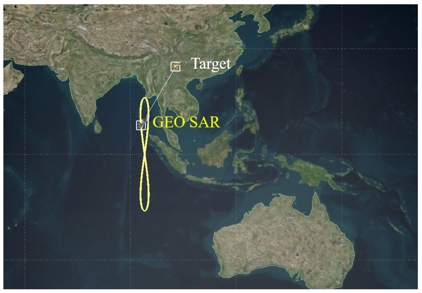
Figure 6 illustrates the orbital path of the satellite based on the orbital elements provided in Table 2. The target in Figure 6 is the central point of the observed target array set by the simulation, located at 102.83 degrees east longitude and 24.88 degrees north latitude. The target array consists of nine point targets with an array size of 7 × 7 km.
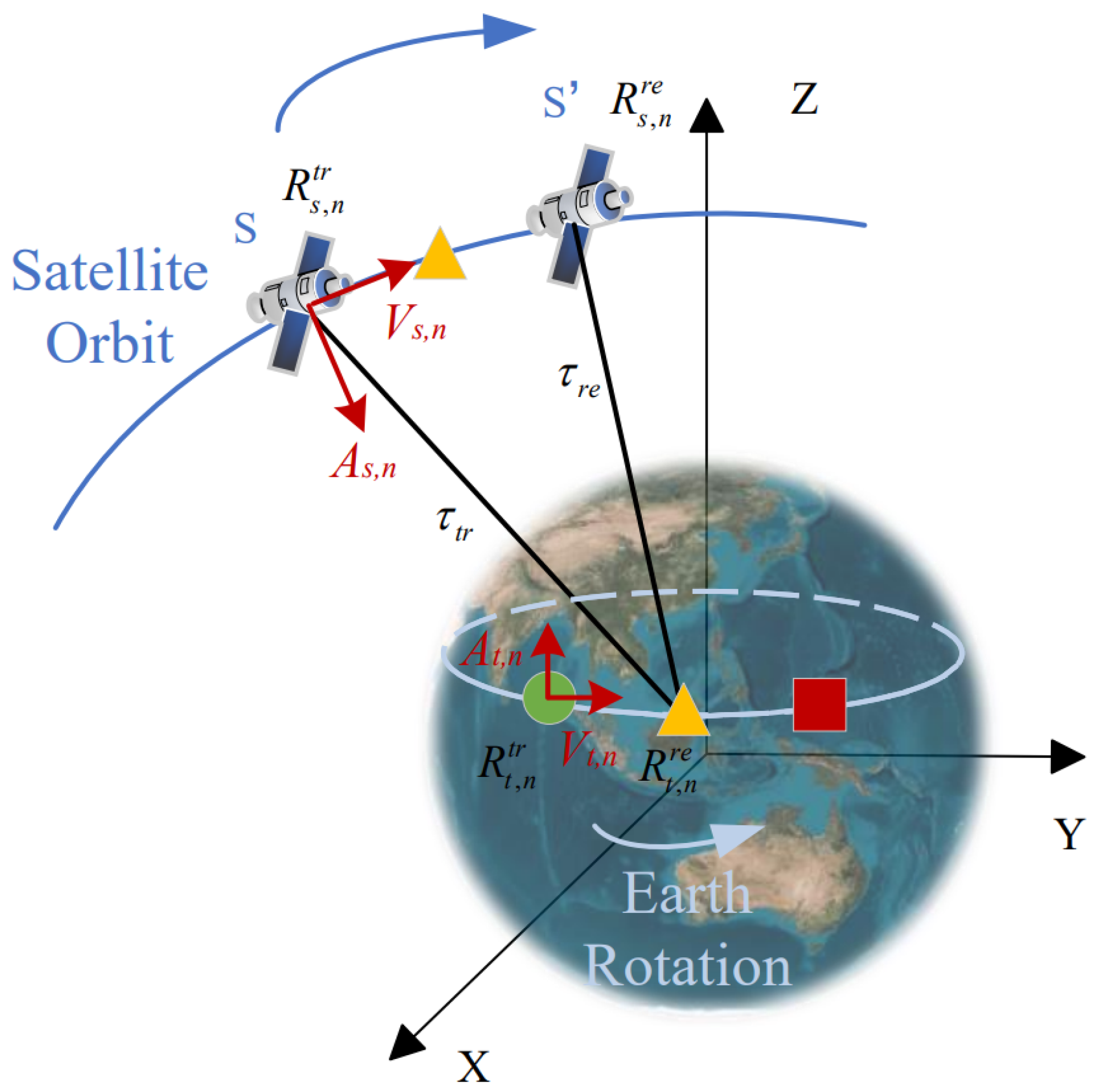
The SAR satellite operates in a geosynchronous orbit at a height of 36,000 km. The separation between the transmitter and receiver is more than 1 km, and this separation phenomenon intensifies with the increasing imaging off-nadir angle of the GEO SAR. The curvature effect of the satellite orbit should be taken into account, as the motion of the target caused by the Earth’s rotation is influenced by the Earth’s curvature. Directly calculating the slant range without considering the orbit curvature effect, the Earth’s curvature impact, and the elliptical shape of the satellite orbit can introduce errors in the precise slant range modeling of the geosynchronous SAR. These errors are magnified with an increased synthetic aperture time, larger off-nadir imaging angles, and greater satellite orbit eccentricity. The magnitude of slant range errors for different azimuth samples is illustrated in the graph shown in Figure 7. 
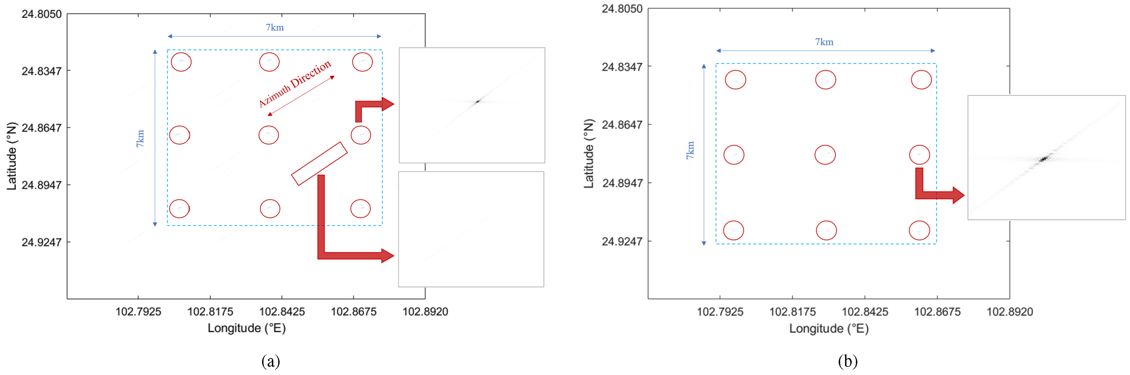
Figure 8a represents the imaging results obtained without accounting for the satellite and target motion during the pulse transmission and reception process. As a result, each point target in the target array showed significant defocusing in the azimuth direction and experienced a displacement.
A Precise Slant Range Model was constructed using the satellite’s velocity and acceleration to describe the curvature motion of the radar along the satellite orbit and the circular motion of the target caused by the Earth’s rotation during the signal’s travel time from transmission to reception. The imaging results of one of the point targets based on the PSRM are shown in 
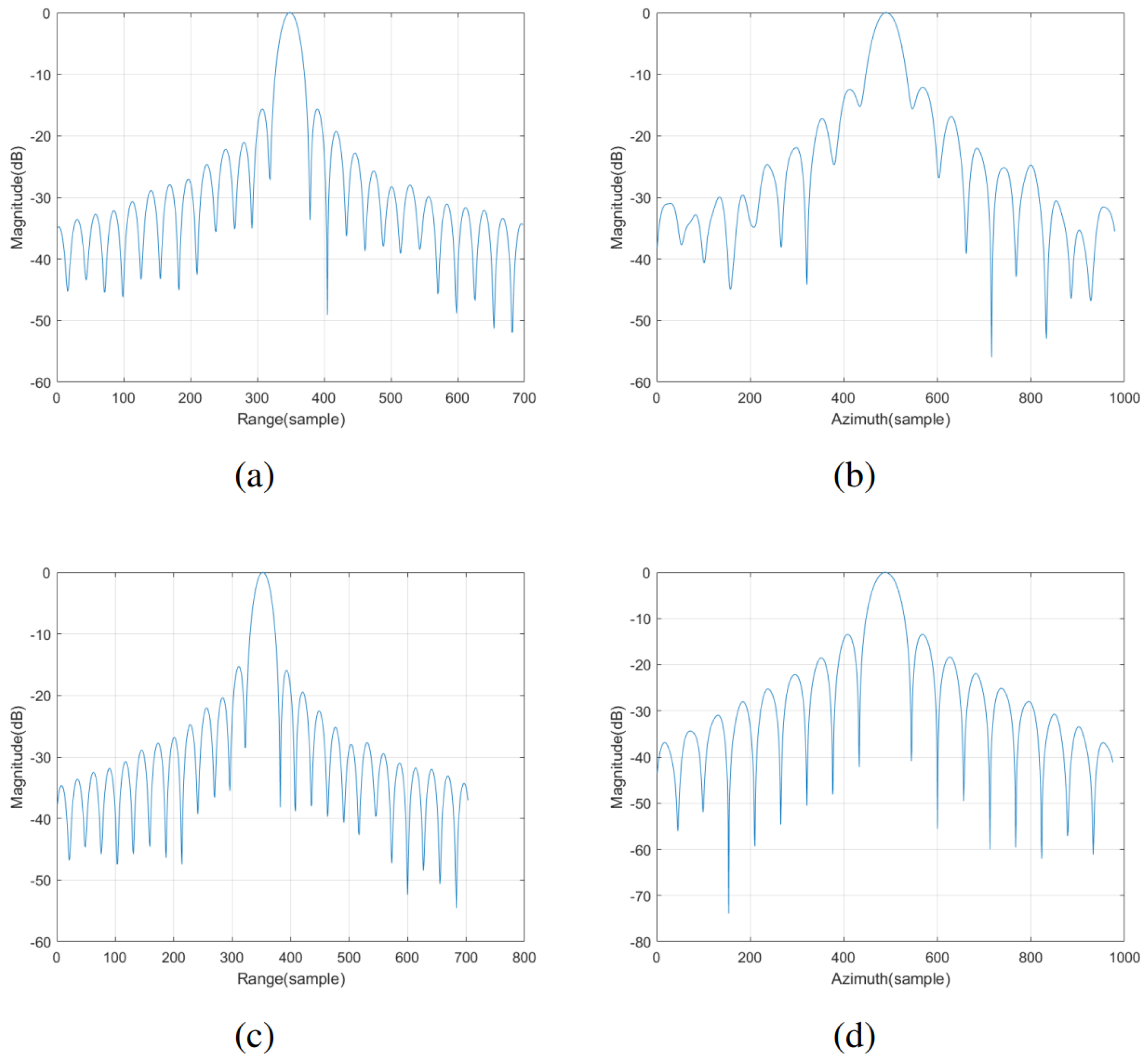
Figure 8b. The azimuth and range profiles are presented in Figure 9. A significant improvement in the focusing quality of the point targets was observed compared to the direct calculation of the slant range. The peak sidelobe ratio and integrated sidelobe ratio of the focused point targets are provided in Table 3. The Precise Slant Range Model considered the motion of the satellite and target points in the GEO SAR “Stop-and-Go” assumption errors, enabling a more accurate calculation of the slant range between the satellite and target and enhancing the imaging quality.

6.2. Interpolation Method Selection Validation

The key to the proposed AEBP algorithm is utilizing interpolation instead of directly calculating the slant range for each grid point. By employing interpolation methods, the computational burden of three-dimensional array slant range calculation is reduced, leading to a significant improvement in computational efficiency. There are various interpolation algorithms available, and the choice of interpolation method is crucial. In this study, we considered three closely related interpolation methods:
(1)
Nearest-Neighbor Interpolation: The numerical value of the nearest neighboring grid point is replaced with that of the grid control point.
(2)
Bilinear Interpolation: This method extends the linear interpolation of an interpolation function with two variables. The core idea is to perform a linear interpolation in each direction separately.
(3)
Bicubic Interpolation: Bicubic interpolation is a sophisticated method that utilizes the numerical values of the 16 surrounding points to calculate a cubic interpolation. It considers the influence of the four adjacent points as well as the variation rates between neighboring points.
To determine the optimal interpolation method, an experiment was conducted using a grid of size 3000 × 3000 with 1 m grid spacing. The target point was positioned at the grid’s center. The slant range between the satellite and each grid point was calculated using the three aforementioned interpolation methods, as well as the direct slant range calculation method. The errors in the slant range between the three interpolation methods and the directly calculated range were measured and are illustrated in Figure 10. The computation time and maximum slant range error are presented in Table 4.
The Nearest-Neighbor Interpolation method demonstrated the fastest calculation speed but introduced larger slant range errors, resulting in lower image quality. Bilinear Interpolation, which employed 4 ( 2 × 2 ) grid points to compute a new point, performed slightly worse than Bicubic Interpolation but offered a faster calculation speed. Bicubic Interpolation, on the other hand, employed 16 ( 4 × 4 ) grid points to compute a new point, resulting in the smallest slant range error and superior image quality. However, this advantage was accompanied by a significant increase in computational load. Therefore, Bilinear Interpolation was selected as the method for efficiently computing the slant range of grid points in the AEBP algorithm.

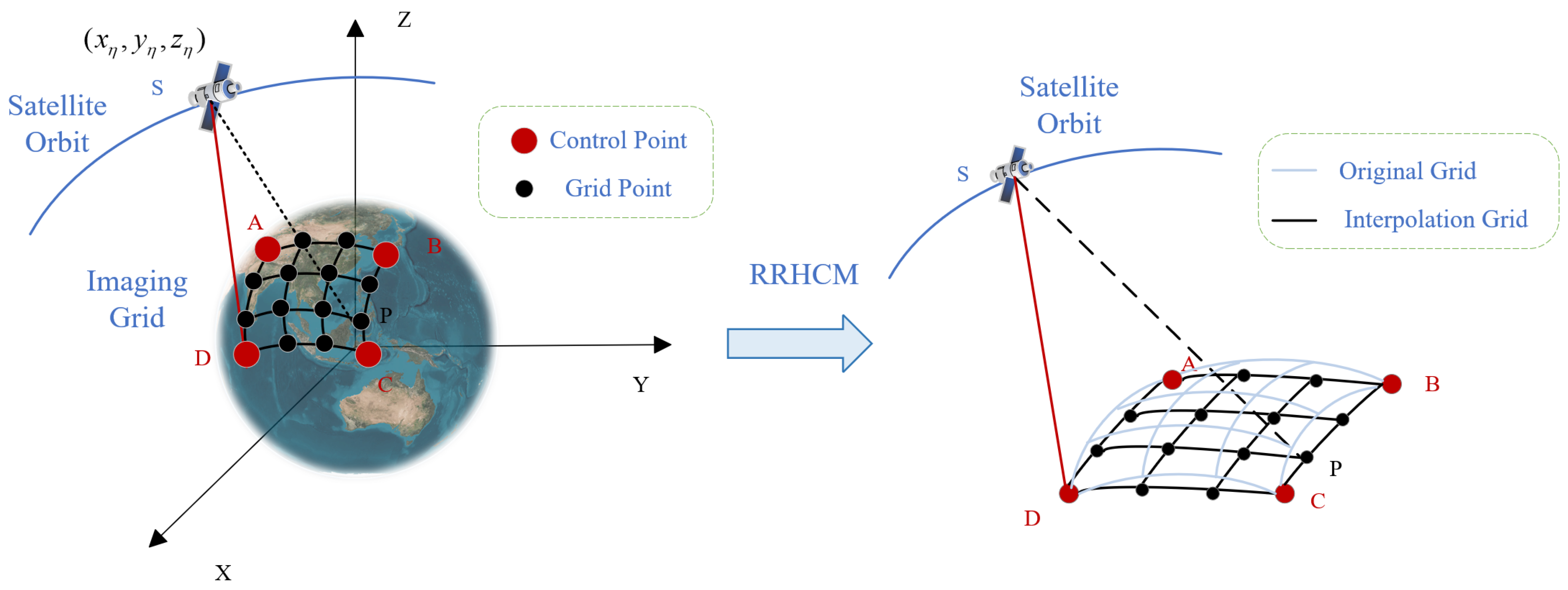
6.3. Validation of AEBP Based on PSRM and RRHCM

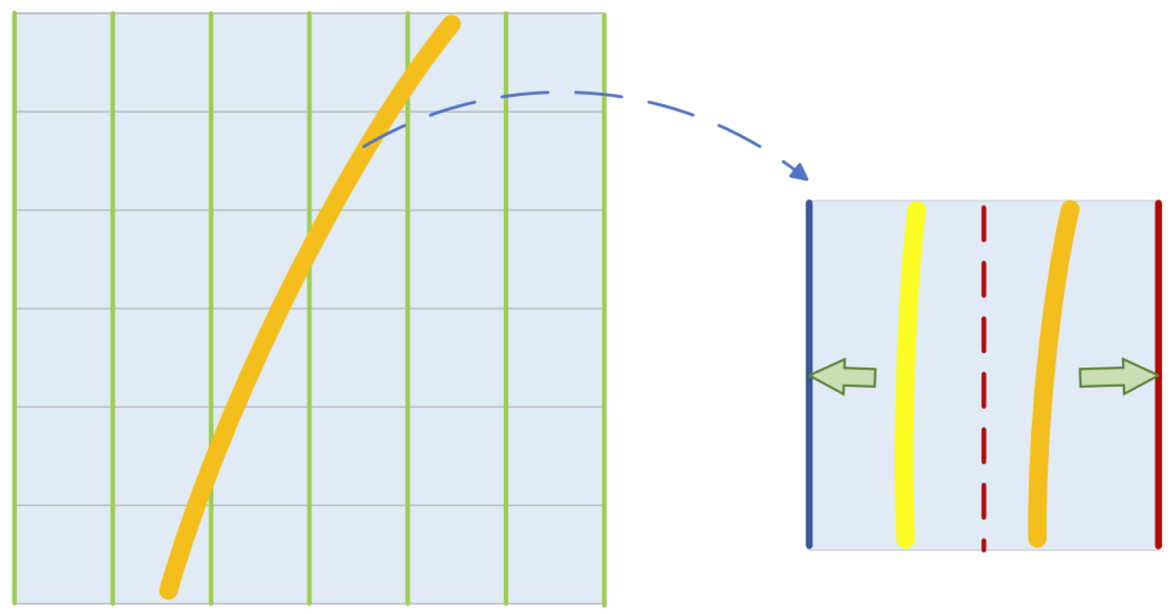
GEO SAR for Earth observation possesses the characteristics of frequent revisits, broad coverage, and the ability to conduct focused observations of particular areas. To prevent the occurrence of blind zones, the receiving pulse window of spaceborne Synthetic Aperture Radar (SAR) must be distinct from the transmitting pulse window. A higher resolution and slant angle lead to an increased synthetic aperture time and range cell migration (RCM). In certain azimuth positions, specific beam placements in the system design must be chosen near blind zones. However, due to the influence of range cell migration (RCM), echo pulses received from these positions may surpass the receiving window. Conversely, reducing the width of the range swath is necessary to ensure the complete reception of all echo pulses. To overcome these challenges and mitigate the influence of range cell migration (RCM) on the range swath, GEO SAR utilizes a variable Pulse Repetition Frequency (PRF) technique. The continuous modification of the PRF results in a more dispersed distribution of blind zones. The positions of the blind zones and the choice of PRF are deterministically linked. A fixed PRF would result in a fixed distribution of blind zones, while continuous PRF variation causes the blind zone positions to change along the azimuth direction. The combination of the variable PRF technique and high-resolution oblique SAR staring mode in satellite-borne SAR ensures a reduced data volume for the echo while maintaining the range swath width.
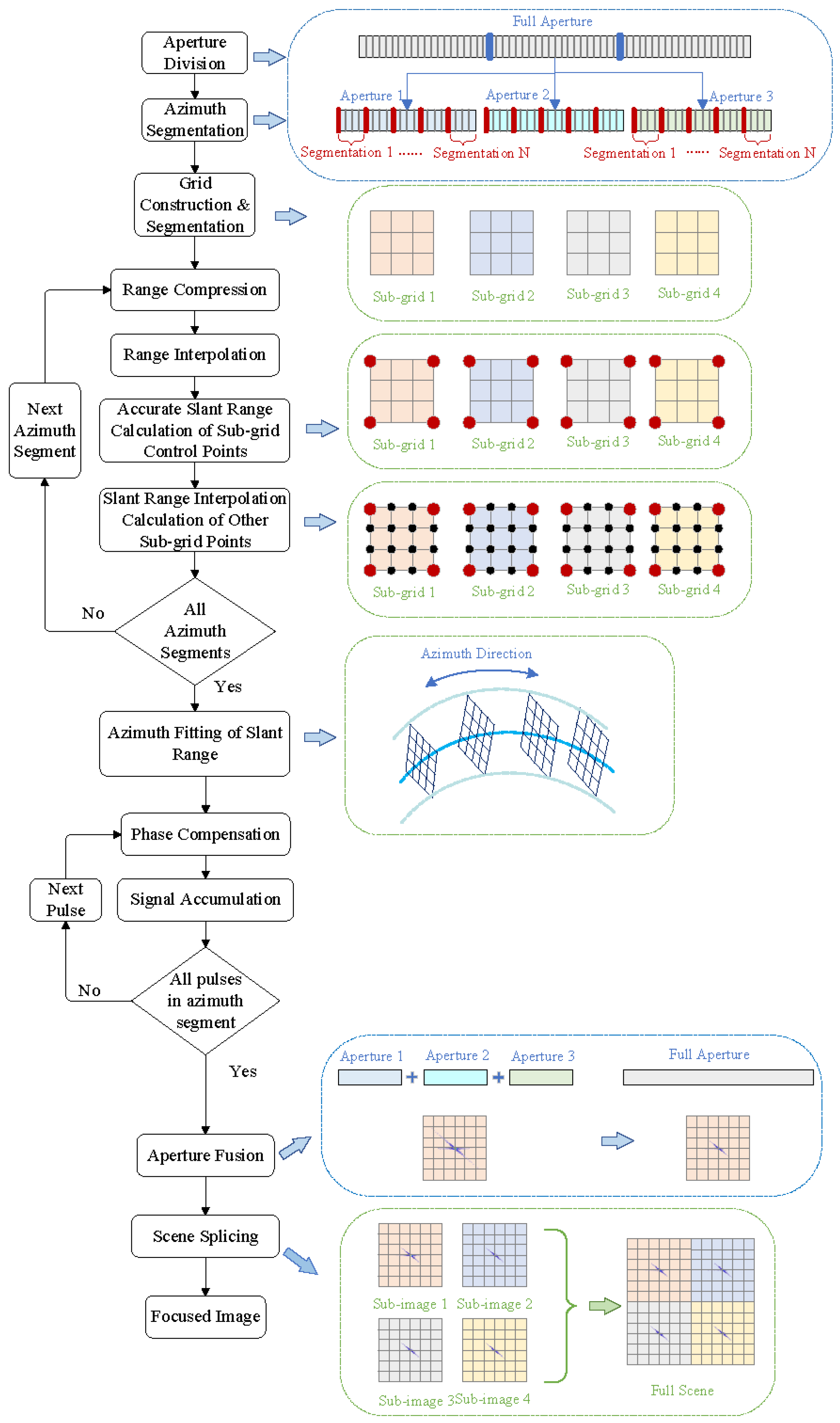
The GEO SAR staring mode adopts a segmented variable PRF technique. In the variable PRF SAR, the echo signal is non-uniform solely in the azimuth direction. By applying the BP algorithm to echo signals obtained with the variable PRF, data focusing is directly accomplished in the time domain. The BP algorithm can be regarded as a coherent pulse-by-pulse accumulation process of point targets in the scene along the azimuth direction in the time domain. This overcomes the requirement for uniform sampling in the azimuth direction, as necessitated by frequency-domain algorithms. However, the computational complexity of the BP algorithm scales proportionally to the product of the number of pixels within the imaging area and the number of azimuth sampling points in the echo. Consequently, the BP algorithm entails a significant computational burden. To tackle this issue, according to the variation pattern of the PRF, the subaperture decomposition technique is employed. The BP algorithm is applied within each subaperture to generate a coarse-resolution image, while coherent synthesis between subapertures is carried out to achieve a high resolution. Table 5 presents the pulse repetition time (PRT), number of sustained pulses, and acquisition window width for each of the three subapertures.
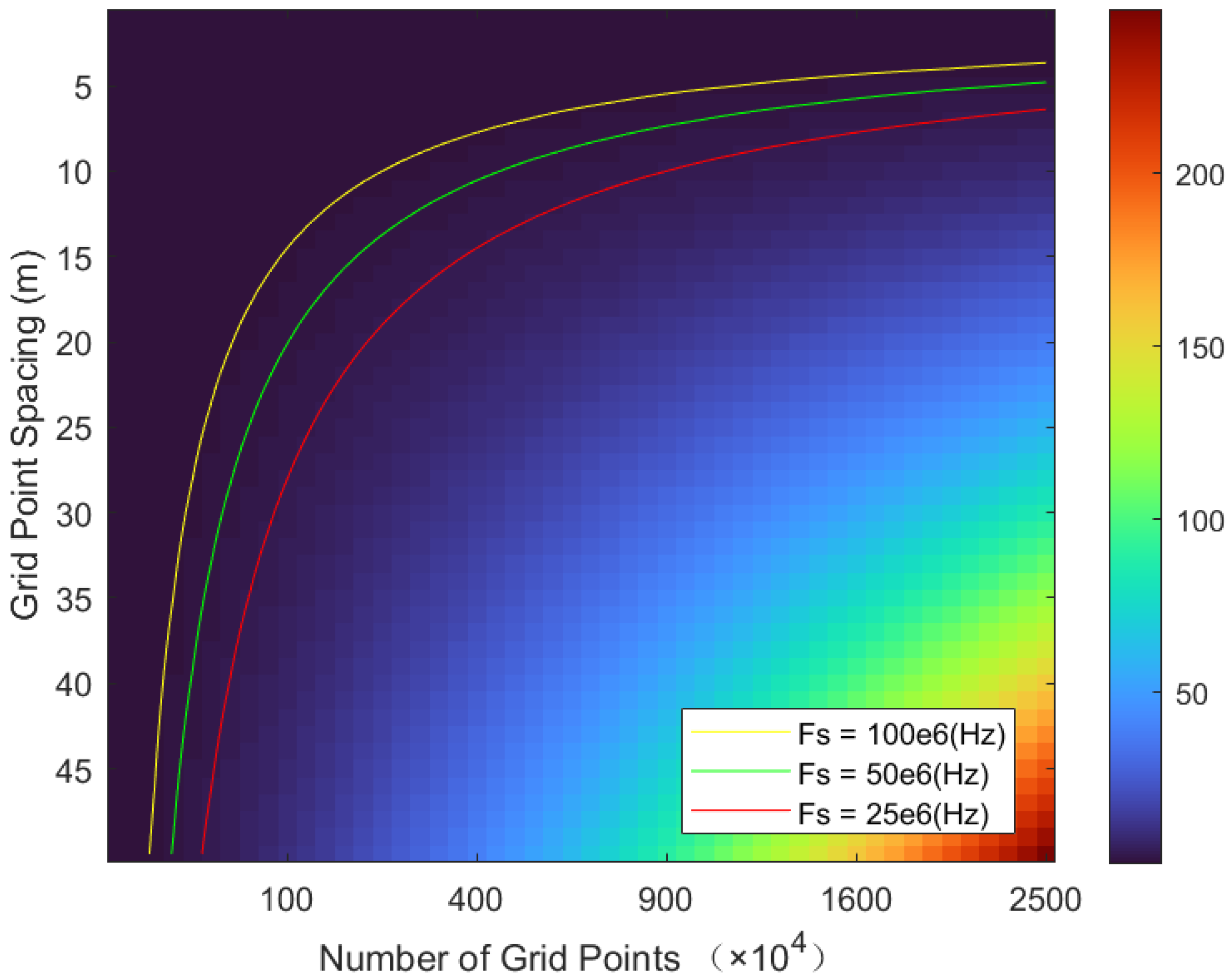
Subsequently, it is crucial to ascertain the suitable grid size and grid spacing. Excessive grid points or an enlarged grid spacing can amplify the error between the interpolated slant range and the precise slant range. As a consequence, the accuracy of the echo signals in the back-projection process is compromised, resulting in scattered point targets and the degradation of image quality. Conversely, an inadequate number of grid points or a reduced grid spacing may result in an excessive quantity of subgrids, consequently prolonging the processing time for subgrid imaging. Thus, it is crucial to opt for a larger grid size without compromising image quality. To guarantee image quality, it is necessary for the back-projection echo values to be accurate, which means that the range error at the grid points should be smaller than a range gate. This range error is primarily related to the range sampling rate expressed as Fs. Since the range errors at different grid points within the grid are not the same, the average range error of all grid points in the grid can be used to assess the range error for that particular grid.
Figure 11 illustrates the analysis of the average range error under different grid sizes and grid spacings. As more grid points are used and the grid spacing increases, the average range error of the grid increases, resulting in poorer image quality in the respective grid. Additionally, Figure 11 depicts the range gate variation for different range sampling rates. The upper-left portion of the curve indicates that the grid range error is smaller than the range gate for that particular range sampling rate. In this case, the back-projection echo values at the grid points within that grid are accurate, ensuring that the grid’s image quality remains unaffected. Therefore, Figure 11 can be used to select suitable grid sizes and spacing for constructing subgrids.
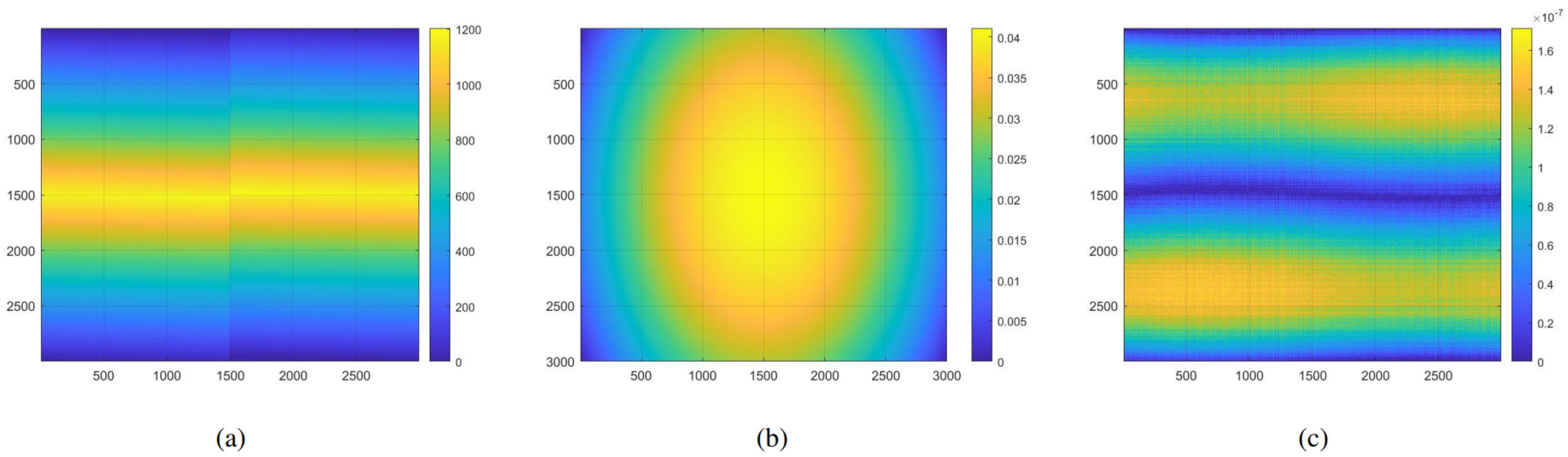
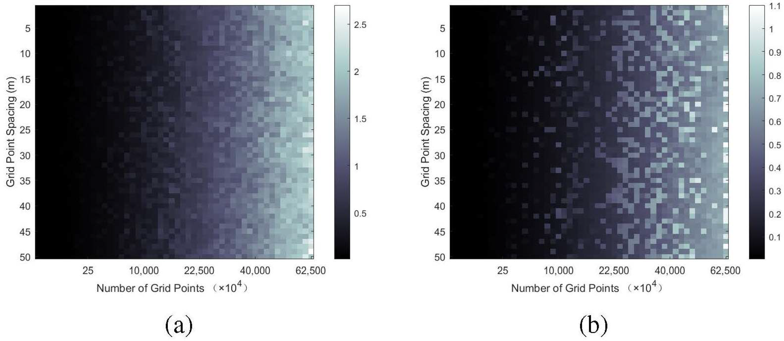
We also examined the factors affecting the slant range computation time. Figure 12 showcases the time needed to compute the slant range for all grid points at a specific azimuth moment, considering different grid sizes and grid spacing values. The pixel values of the image are measured in seconds. In the graph on the left, the slant range is directly calculated, while in the graph on the right, the RRHCM is used. It can be observed that the slant range computation time is not affected by the grid size but instead depends on the number of grid points. As the number of grid points increases and the grid size becomes larger, more time is required to compute the slant range values.
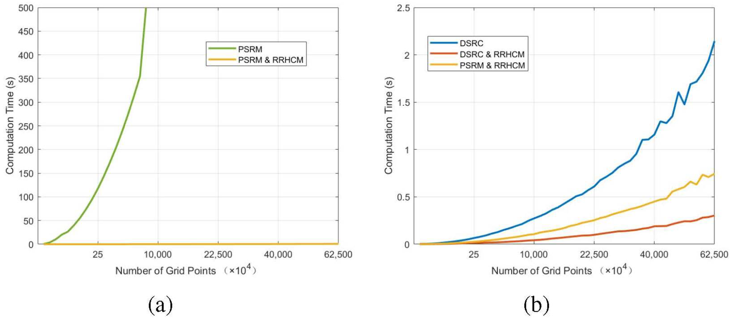
With a constant grid spacing of 4 m, we compared the time required by four different slant range methods for varying numbers of grid points, as shown in Figure 13. The DSRC method represents the direct calculation of slant range, PSRM represents the Precise Slant Range Model, DSRC & RRHCM represents direct slant range calculation for control points using the Rapid Range History Construction Method, and PSRM & RRHCM represents the use of the Precise Slant Range Model for control points with the Rapid Range History Construction Method applied for the rest of the grid points. As shown in the graph on the left, there was a significant increase in the time needed for PSRM to compute the grid slant range. However, using the Rapid Range History Construction Method could reduce the computation time. When compared to PSRM, the time required for PSRM & RRHCM remained nearly constant. In the graph on the right, DSRC & RRHCM exhibits a slower increase rate compared to DSRC, indicating that the Rapid Range History Construction Method also reduced the time needed for direct slant range calculation. PSRM & RRHCM required nearly half the computation time of DSRC but a slightly longer computation time than DSRC & RRHCM. In conclusion, the Rapid Range History Construction Method could effectively reduce the computation time for slant range calculation, decrease the computational workload, and consequently shorten the processing time for imaging, thereby enhancing the imaging timeliness.
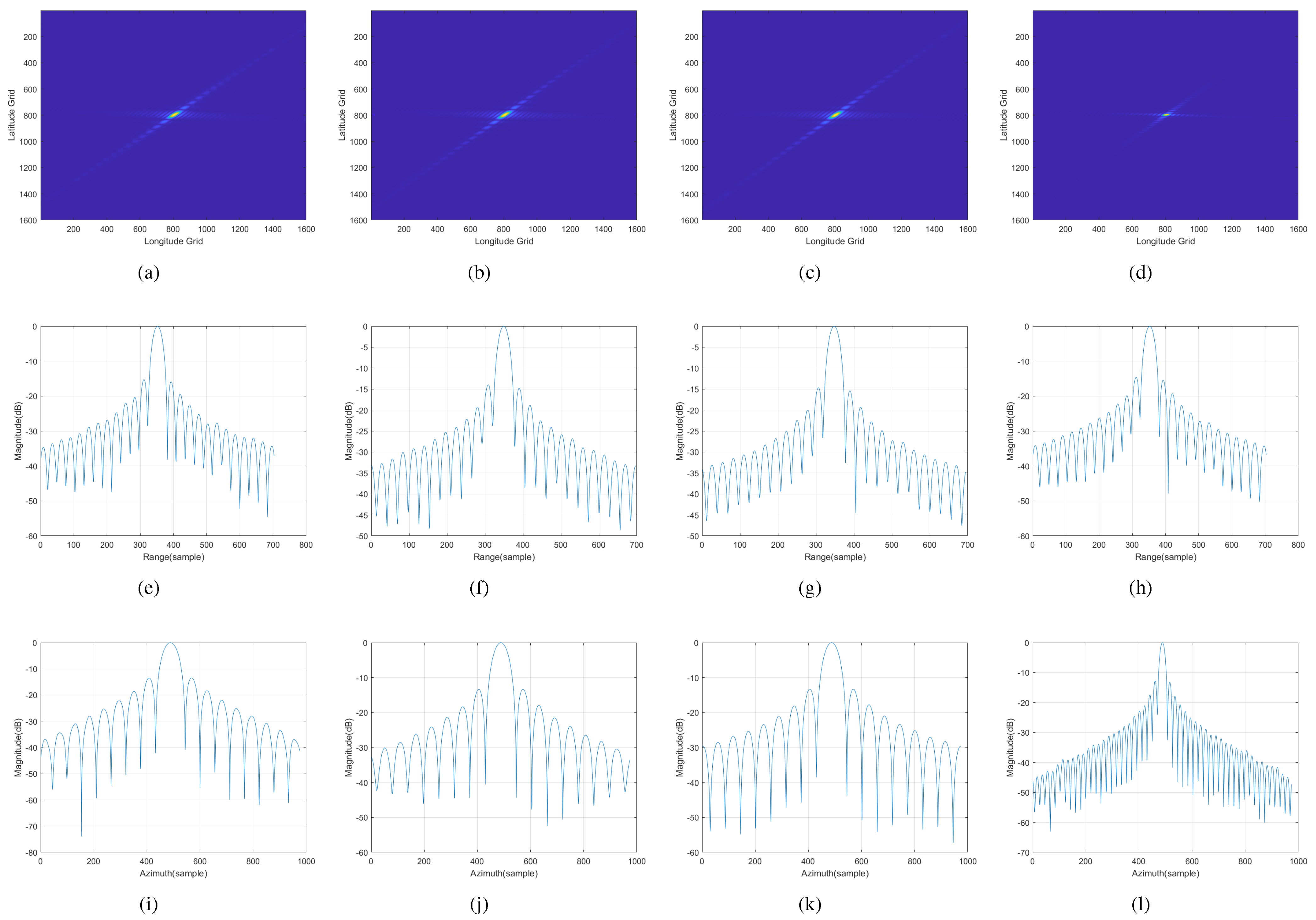
Next, we analyzed the imaging quality of the AEBP algorithm using the Precise Slant Range Model and the Rapid Range History Construction Method. The grid was 2500 × 2500 
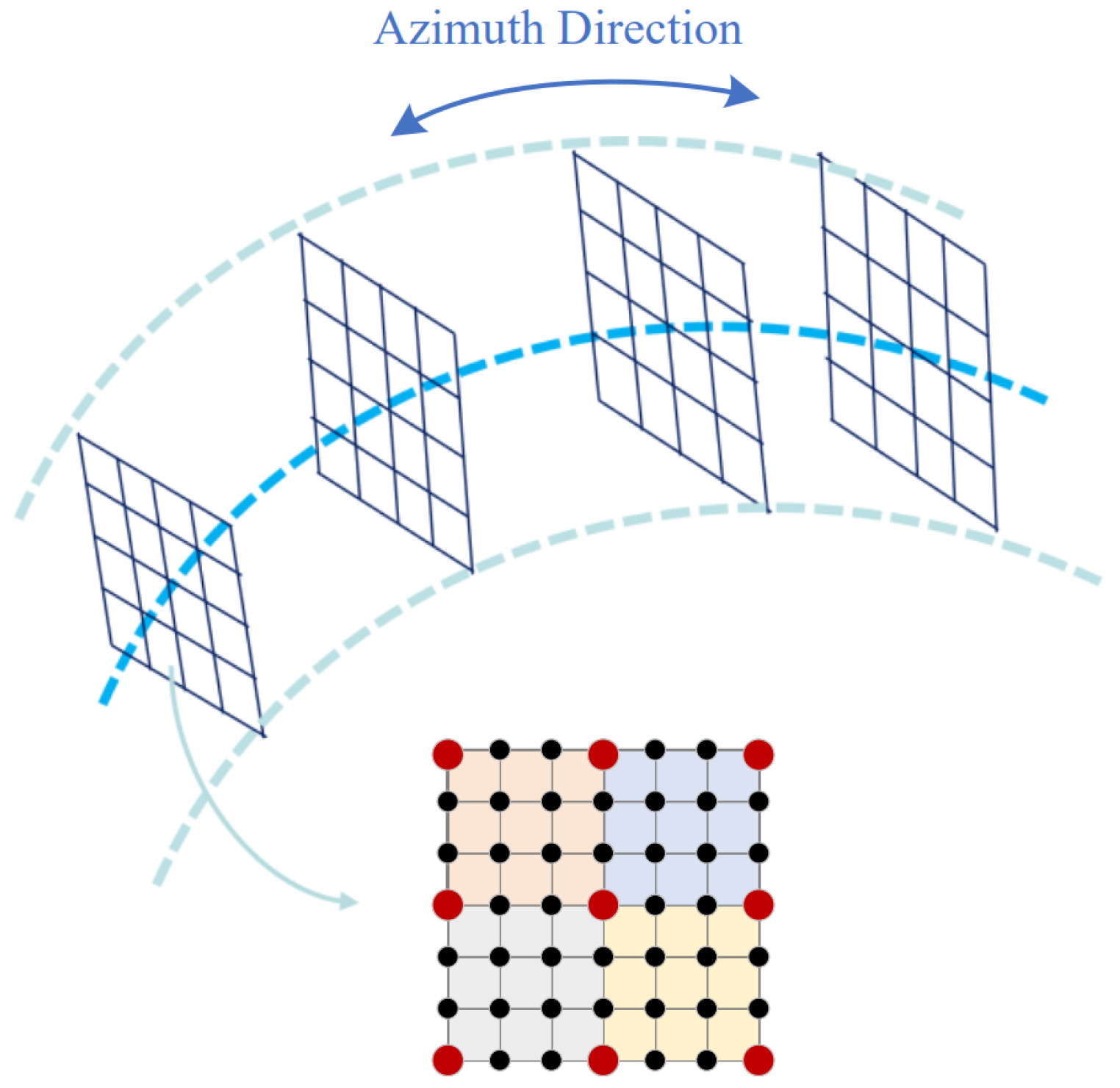
with a spacing of 4 m. The point target was positioned at the center of the grid. Imaging was conducted separately for three subapertures. The slant range for the control points of the grid was calculated using the Precise Slant Range Model, while the slant range for the remaining grid points was interpolated using the RRCHM. The imaging results for the three subapertures and their fusion are illustrated in Figure 14. The first row shows the focused image of the point target, while the second and third rows display the range direction envelope and azimuth direction envelope, respectively. The quality analysis of the point target imaging and the reduced time (RT) for imaging are summarized in Table 6. The peak sidelobe ratio (PSR) and integrated sidelobe ratio (ISR) (normalized to the theoretical value) were −13.26 dB and −9.68 dB, respectively. The RT value was obtained by comparing the time taken to shorten the experiment with the time taken to directly calculate the subaperture grid point slant range. A higher RT indicates that the AEBP algorithm could save more time. PSRM represents the focal results of point targets obtained by calculating the slant ranges of all grid points in the azimuth direction using the Precise Slant Range Model. Conversely, PSRM & RRHCM represents the focal results of point targets obtained using the Precise Slant Range Model and the Rapid Range History Construction Method. It is evident that the imaging results obtained using the Precise Slant Range Model exhibited excellent imaging performance. The parallel processing of subapertures significantly reduced the imaging time, while the coherent fusion of subapertures enhanced the azimuth resolution. The RRCHM further improved the computational efficiency. The proposed algorithm ensured high imaging quality and enhanced the timeliness of imaging processing. It could also be combined with the aperture segmentation approach.
The fusion of three subapertures improved the azimuth resolution, resulting in a high-precision image, as shown in Figure 14. Table 6 presents an analysis of the image quality. PSRM represents the focal results of point targets obtained by calculating the slant ranges of all grid points in the azimuth direction using the Precise Slant Range Model. PSRM & RRHCM represents the focal results of point targets obtained using both the Precise Slant Range Model and the Rapid Range History Construction Method. The imaging results obtained using the Precise Slant Range Model demonstrated excellent imaging performance. The parallel processing of subapertures reduced the imaging time, while the coherent fusion of subapertures enhanced the azimuth resolution. Furthermore, the RRCHM improved the computational efficiency, ensuring high-quality imaging and timely processing.

6.4. Performance Evaluation

The proposed AEBP algorithm, when combined with the Precise Slant Range Model (PSRM), exhibited enhanced imaging quality compared to traditional BP algorithms. PSRM provides a more accurate estimation of slant range, which contributes to improved imaging quality. By incorporating the velocity and acceleration of both the satellite and target, PSRM ensures that slant range values are computed with higher precision. Utilizing the precise slant range values provided by PSRM, the AEBP algorithm can more effectively focus the radar signals, resulting in sharper and more detailed images.
Additionally, the Rapid Range History Construction Method (RRHCM) significantly improves the imaging speed of the AEBP algorithm. RRHCM offers a more expedient approach to computing slant range. Although it may introduce some trade-offs in terms of precision compared to PSRM, it still produces satisfactory imaging quality. By significantly reducing the computation time for non-control grid points, the fast calculation method enables faster image generation without compromising the overall quality. Additionally, RRHCM is not limited by the type of coordinate system used. The introduction of previous methods and experimental validation were conducted in the Cartesian coordinate system. However, for the polar coordinate system, it was shown that the RRHCM still exhibited promising performance, as demonstrated in Table 7. RT RHC represents the time reduction for constructing the grid range history, while RT BPO represents the reduced time for the back-projection operation.
The combination of the PSRM and RRCHM enables enhanced timeliness and efficiency in generating high-quality radar images. The algorithm effectively handles large datasets and complex scenes, making it suitable for real-time applications and scenarios that require rapid image processing.
In summary, the Accurate and Efficient Back-Projection (AEBP) algorithm, based on the Precise Slant Range Model (PSRM) and the Rapid Range History Construction Method (RRHCM), provides superior imaging quality and speed compared to traditional BP algorithms and fast BP algorithms. The accuracy of the slant range model contributes to sharper images, while the fast calculation method ensures efficient processing without sacrificing quality. This combination makes the algorithm well-suited for real-time imaging tasks that demand both accuracy and speed. The proposed AEBP algorithm optimizes each back-projection operation and the construction of the grid range history, independent of the coordinate system used. It does not affect the performance of subaperture fusion and exhibits strong universality. Consequently, the AEBP algorithm can be integrated with existing fast BP algorithms to reduce the speed of back-projection during the fast BP imaging process, thereby further enhancing the imaging speed of fast BP.
The current implementation of the proposed method is limited to uniform imaging grids. These limitations restrict the division of imaging grids. However, due to grid approximation, there may be errors in the calculated slant ranges. The proposed method does not incorporate range error compensation. Thus, the influence of range error can only be managed by selecting a smaller grid size for imaging. Subsequently, we will further refine the Rapid Range History Construction Method to enable its applicability to non-uniform imaging grids. Additionally, we will investigate a compensation method to correct the slant range error. Moreover, the validation was limited to simulation targets. Subsequently, we will also apply the proposed method to real data for further evaluation.

7. Conclusions

This paper presented the Accurate and Efficient Back-Projection (AEBP) algorithm, an imaging algorithm designed for GEO SAR. The algorithm utilizes the Precise Slant Range Model (PSRM) and the Rapid Range History Construction Method (RRHCM) as its foundation.
In this study, the PSRM was developed to compensate for “Stop-and-Go” assumption errors in the time domain, considering both the curved motion along the satellite orbit and the circular motion caused by the Earth’s rotation. Additionally, we proposed the RRHCM, which utilizes interpolation to generate the range history for all grid points directly. This approach effectively reduces the computational complexity associated with the three-dimensional array of range history. Following a theoretical analysis and experimental comparisons of different interpolation methods, we concluded that Bilinear Interpolation is the most suitable method for approximating the slant range within the grid. We performed an analysis to evaluate the RRHCM in terms of its error and its impact on the final imaging results. Based on the error analysis findings, we proposed a set of criteria for constructing the imaging grid and validated them through simulations.
In conclusion, this paper introduced the AEBP algorithm for GEO SAR imaging. The algorithm was developed by utilizing the PSRM and the RRHCM. It includes preprocessing, imaging processing, and postprocessing stages. The proposed AEBP imaging algorithm separates the calculation of slant range from the processing of azimuth pulses. Initially, the range history for the entire azimuth is constructed, followed by the accumulation of signals at various grid points for different moments in the azimuth. The PSRM is used to calculate the range at the four control points of the grid, while the RRHCM is used for the remaining grid points. Utilizing the PSRM ensures high precision in the range history, thus enhancing image quality. Additionally, the RRHCM improves computational speed while maintaining image quality. Finally, the proposed imaging algorithm was validated through simulations using the parameters of the GEO SAR system. A comparative analysis was conducted to evaluate both the image quality and computational speed. The experimental results clearly demonstrated that the proposed AEBP algorithm achieved high precision and efficiency in GEO SAR imaging processing. The proposed algorithm optimizes the back-projection operation, displaying strong versatility and the ability to be integrated with other fast BP algorithms, thus further enhancing the efficiency of fast BP imaging.

Author Contributions

Conceptualization, Y.W. and L.H.; methodology, Y.W.; software, L.H.; validation, Y.W. and L.H.; formal analysis, Y.W.; investigation, Y.W.; resources, L.H.; data curation, L.H.; writing—original draft preparation, Y.W.; writing—review and editing, Y.W.; visualization, B.Z.; supervision, X.W., X.Q.; project administration, L.H.; funding acquisition, L.H. All authors have read and agreed to the published version of the manuscript.

Funding

This research was funded by the Youth Innovation Promotion Association No. 2019127, Chinese Academy of Sciences.

Data Availability Statement

Data available on request from the authors. The data that support the findings of this study are available from the corresponding author upon reasonable request.

Conflicts of Interest

The authors declare no conflict of interest.

References

  1. Bruno, D.; Hobbs, S.E.; Ottavianelli, G. Geosynchronous synthetic aperture radar: Concept design, properties and possible applications. Acta Astronaut. 2006, 59, 149–156. [Google Scholar] [CrossRef]
  2. Xu, H.; Huang, L.; Qiu, X.; Han, B.; Zhong, L.; Meng, D. A new geosynchronous SAR constellation and its signal characteristics. IEEE Access 2019, 7, 101539–101551. [Google Scholar] [CrossRef]
  3. Mittermayer, J.; Moreira, A.; Loffeld, O. Spotlight SAR data processing using the frequency scaling algorithm. IEEE Trans. Geosci. Remote Sens. 1999, 37, 2198–2214. [Google Scholar] [CrossRef]
  4. Bamler, R. A comparison of range-Doppler and wavenumber domain SAR focusing algorithms. IEEE Trans. Geosci. Remote Sens. 1992, 30, 706–713. [Google Scholar] [CrossRef]
  5. Raney, R.K.; Runge, H.; Bamler, R.; Cumming, I.G.; Wong, F.H. Precision SAR processing using chirp scaling. IEEE Trans. Geosci. Remote Sens. 1994, 32, 786–799. [Google Scholar] [CrossRef]
  6. Wong, F.; Yeo, T.S. New applications of nonlinear chirp scaling in SAR data processing. IEEE Trans. Geosci. Remote Sens. 2001, 39, 946–953. [Google Scholar] [CrossRef]
  7. Hu, C.; Long, T.; Liu, Z.; Zeng, T.; Tian, Y. An improved frequency domain focusing method in geosynchronous SAR. IEEE Trans. Geosci. Remote Sens. 2013, 52, 5514–5528. [Google Scholar]
  8. Hu, B.; Jiang, Y.; Zhang, S.; Zhang, Y.; Yeo, T.S. Generalized omega-K algorithm for geosynchronous SAR image formation. IEEE Geosci. Remote Sens. Lett. 2015, 12, 2286–2290. [Google Scholar] [CrossRef]
  9. Sun, G.C.; Xing, M.; Wang, Y.; Yang, J.; Bao, Z. A 2-D space-variant chirp scaling algorithm based on the RCM equalization and subband synthesis to process geosynchronous SAR data. IEEE Trans. Geosci. Remote Sens. 2013, 52, 4868–4880. [Google Scholar]
  10. Li, D.; Wu, M.; Sun, Z.; He, F.; Dong, Z. Modeling and processing of two-dimensional spatial-variant geosynchronous SAR data. IEEE J. Sel. Top. Appl. Earth Obs. Remote Sens. 2015, 8, 3999–4009. [Google Scholar] [CrossRef]
  11. Zhang, T.; Ding, Z.; Tian, W.; Zeng, T.; Yin, W. A 2-D nonlinear chirp scaling algorithm for high squint GEO SAR imaging based on optimal azimuth polynomial compensation. IEEE J. Sel. Top. Appl. Earth Obs. Remote Sens. 2017, 10, 5724–5735. [Google Scholar] [CrossRef]
  12. Chen, J.; Sun, G.C.; Wang, Y.; Xing, M.; Li, Z.; Zhang, Q.; Liu, L.; Dai, C. A TSVD-NCS algorithm in range-Doppler domain for geosynchronous synthetic aperture radar. IEEE Geosci. Remote Sens. Lett. 2016, 13, 1631–1635. [Google Scholar] [CrossRef]
  13. Hu, C.; Liu, Z.; Long, T. An improved CS algorithm based on the curved trajectory in geosynchronous SAR. IEEE J. Sel. Top. Appl. Earth Obs. Remote Sens. 2012, 5, 795–808. [Google Scholar] [CrossRef]
  14. Munson, D.C.; O’Brien, J.D.; Jenkins, W.K. A tomographic formulation of spotlight-mode synthetic aperture radar. Proc. IEEE 1983, 71, 917–925. [Google Scholar] [CrossRef]
  15. Chen, J.; Sun, G.C.; Xing, M.; Yang, J.; Li, Z.; Jing, G. A two-dimensional beam-steering method to simultaneously consider Doppler centroid and ground observation in GEOSAR. IEEE J. Sel. Top. Appl. Earth Obs. Remote Sens. 2016, 10, 161–167. [Google Scholar] [CrossRef]
  16. Li, Z.; Li, C.; Yu, Z.; Zhou, J.; Chen, J. Back projection algorithm for high resolution GEO-SAR image formation. In Proceedings of the 2011 IEEE International Geoscience and Remote Sensing Symposium, Vancouver, BC, Canada, 24–29 July 2011; IEEE: Piscataway, NJ, USA, 2011; pp. 336–339. [Google Scholar]
  17. Ding, Y.; Munson, D.J. A fast back-projection algorithm for bistatic SAR imaging. In Proceedings of the International Conference on Image Processing, Rochester, NY, USA, 22–25 September 2002; IEEE: Piscataway, NJ, USA, 2002; Volume 2, p. II. [Google Scholar]
  18. Bie, B.; Xing, M.; Xia, X.G.; Sun, G.C.; Liang, Y.; Jing, G.; Wei, T.; Yu, Y. A frequency domain backprojection algorithm based on local cartesian coordinate and subregion range migration correction for high-squint SAR mounted on maneuvering platforms. IEEE Trans. Geosci. Remote Sens. 2018, 56, 7086–7101. [Google Scholar] [CrossRef]
  19. Juan, C.; Jintao, X.; Yulin, H.; Jiangyu, Y. Research on a novel fast backprojection algorithm for stripmap bistatic SAR imaging. In Proceedings of the 2007 1st Asian and Pacific Conference on Synthetic Aperture Radar, Huangshan, China, 5–9 November 2007; IEEE: Piscataway, NJ, USA, 2007; pp. 622–625. [Google Scholar]
  20. Hu, C.; Long, T.; Zeng, T.; Liu, F.; Liu, Z. The accurate focusing and resolution analysis method in geosynchronous SAR. IEEE Trans. Geosci. Remote Sens. 2011, 49, 3548–3563. [Google Scholar] [CrossRef]
  21. An, H.; Wu, J.; Teh, K.C.; Sun, Z.; Yang, J. Geosynchronous spaceborne–airborne bistatic SAR imaging based on fast low-rank and sparse matrices recovery. IEEE Trans. Geosci. Remote Sens. 2021, 60, 5207714. [Google Scholar] [CrossRef]
  22. An, H.; Wu, J.; Teh, K.C.; Sun, Z.; Yang, J. Nonambiguous Image Formation for Low-Earth-Orbit SAR With Geosynchronous Illumination Based on Multireceiving and CAMP. IEEE Trans. Geosci. Remote Sens. 2021, 59, 348–362. [Google Scholar] [CrossRef]
  23. Ulander, L.M.; Hellsten, H.; Stenstrom, G. Synthetic-aperture radar processing using fast factorized back-projection. IEEE Trans. Aerosp. Electron. Syst. 2003, 39, 760–776. [Google Scholar] [CrossRef]
  24. Dong, Q.; Sun, G.C.; Yang, Z.; Guo, L.; Xing, M. Cartesian factorized backprojection algorithm for high-resolution spotlight SAR imaging. IEEE Sens. J. 2017, 18, 1160–1168. [Google Scholar] [CrossRef]
  25. Chen, X.; Sun, G.C.; Xing, M.; Li, B.; Yang, J.; Bao, Z. Ground Cartesian back-projection algorithm for high squint diving TOPS SAR imaging. IEEE Trans. Geosci. Remote Sens. 2020, 59, 5812–5827. [Google Scholar] [CrossRef]
  26. Chen, Q.; Liu, W.; Sun, G.C.; Chen, X.; Han, L.; Xing, M. A fast Cartesian back-projection algorithm based on ground surface grid for GEO SAR focusing. IEEE Trans. Geosci. Remote Sens. 2021, 60, 5217114. [Google Scholar] [CrossRef]
  27. Hobbs, S.; Mitchell, C.; Forte, B.; Holley, R.; Snapir, B.; Whittaker, P. System Design for Geosynchronous Synthetic Aperture Radar Missions. IEEE Trans. Geosci. Remote Sens. 2014, 52, 7750–7763. [Google Scholar] [CrossRef]
  28. Long, T.; Dong, X.; Hu, C.; Zeng, T. A New Method of Zero-Doppler Centroid Control in GEO SAR. IEEE Geosci. Remote Sens. Lett. 2011, 8, 512–516. [Google Scholar] [CrossRef]
  29. Hu, C.; Li, Y.; Dong, X.; Wang, R.; Ao, D. Performance Analysis of L-Band Geosynchronous SAR Imaging in the Presence of Ionospheric Scintillation. IEEE Trans. Geosci. Remote Sens. 2017, 55, 159–172. [Google Scholar] [CrossRef]
  30. Hu, C.; Zhang, B.; Dong, X.; Li, Y. Geosynchronous SAR Tomography: Theory and First Experimental Verification Using Beidou IGSO Satellite. IEEE Trans. Geosci. Remote Sens. 2019, 57, 6591–6607. [Google Scholar] [CrossRef]
Figure 1. The relative motion between the satellite and the Earth during the transmission and reception times. The green circle represents the target position at the moment of transmission. The red box represents the target position at the moment of reception. The yellow triangle represents the position of the target and the satellite at the intermediate moment.
Remotesensing 15 05191 g001
Figure 2. Schematic diagram of the Rapid Range History Construction Method.
Remotesensing 15 05191 g002
Figure 3. Flowchart of the proposed Accurate and Efficient BP algorithm. The red dots represent control points and the black dots represent other grid points.
Remotesensing 15 05191 g003
Figure 4. Diagram of the slant range calculation for the proposed Accurate and Efficient BP algorithm. The red dots represent control points and the black dots represent other grid points. The dashed lines indicate azimuth sampling.
Remotesensing 15 05191 g004
Figure 5. Diagram for error analysis in back-projection processing.
Remotesensing 15 05191 g005
Figure 6. Trajectory diagram for GEO SAR based on the orbital elements.
Remotesensing 15 05191 g006
Figure 7. Slant range errors for different azimuth samples.
Remotesensing 15 05191 g007
Figure 8. The imaging results: (a) based on the DSRC, (b) based on the PSRC.
Remotesensing 15 05191 g008
Figure 9. The range and azimuth profiles: (a,b) based on the DSRC, (c,d) based on the PSRC.
Remotesensing 15 05191 g009
Figure 10. The slant range errors of the three interpolation methods and the directly calculated range: (a) Nearest-Neighbor Interpolation, (b) Bilinear Interpolation, (c) Bicubic Interpolation.
Remotesensing 15 05191 g010
Figure 11. An analysis graph depicting the average distance error for different grid sizes under varying grid spacings.
Remotesensing 15 05191 g011
Figure 12. The relationship between the time required for calculating the slant range and the number of grid points and grid spacing: (a) based on DSRC, (b) based on RRHCM.
Remotesensing 15 05191 g012
Figure 13. Comparison charts of computation time based on PSRM, DSRC, and RRHCM: (a) comparison of PSRM and PSRM&RRHCM, (b) comparison of DSRC, DSRC&RRHCM and PSRM&RRHCM.
Remotesensing 15 05191 g013
Figure 14. Contour plots of subaperture imaging: (a,e,i) subaperture 1; (b,f,j) subaperture 2; (c,g,k) subaperture 3; (d,h,l) subaperture fusion.
Remotesensing 15 05191 g014
Table 1. Comparison of computational complexity between traditional BPA and proposed BPA.
AlgorithmComputational Complexity
AdditionMultiplicationSquare Root
Traditional BPA 4 M N L a 3 M N L a M N L a
Proposed BPA 3 M N L a / γ / η 4 M N L a / γ / η 0
Table 2. Simulation parameters of GEO SAR.
Parameter NameValueUnits
Orbital Elements
Semimajor axis42164563.2m
Inclination0.2792450rad
Eccentricity3.724359 × 10 6 -
Longitude of the ascending node3.746894rad
Argument of perihelion5.925221rad
Mean anomaly0.7583125rad
Radar Parameters
Look angle5.335deg
Incidence angle35.10–40.87deg
Squint angle58deg
Chirp bandwidth70MHz
Pulse width500us
Carrier frequency1.25GHz
Synthetic aperture time3600s
Scene Parameters
Central point target longitude102.83°E
Central point target latitude24.88°N
Subgrid width10km
Grid spacing4m
Table 3. Evaluation results of central point target based on DSRM and PSRM.
RangeAzimuth
PSLR (dB)ISLR (dB)3 dB WidthIRW (m)PSLR (dB)ISLR (dB)3 dB WidthIRW (m)
DSRM−15.6429−12.568025.89672.4261−12.0882−9.424350.487813.7756
PSRM−13.3495−10.506925.72862.4104−13.1940−10.397051.103113.0364
Table 4. The computational time and maximum slant range error.
Direct Slant Range CalculationNearest-Neighbor InterpolationBilinear InterpolationBicubic Interpolation
Computational Time (s)0.0358490.015960.0175980.128078
Maximum Range Error (m)-1.2034 × 10 3 0.04111.7136 × 10 7
Table 5. Simulation parameters of three subapertures.
Parameter NameValueUnits
Pulse Repetition TimeSubaperture 15457us
Subaperture 25329us
Subaperture 35102us
Number of Sustained PulsesSubaperture 1109,895-
Subaperture 2112,533-
Subaperture 3117,541-
Acquisition Window WidthSubaperture 12.12992ms
Subaperture 22.08896ms
Subaperture 32.048ms
Table 6. Evaluation results of central point target based on PSRM and RRHCM.
PSRMPSRM & RRHCM
PSLR (dB)ISLR (dB)IRW (m)PSLR (dB)ISLR (dB)IRW (m)RT (%)
Subaperture 1Range−13.3495−10.50692.4104−15.2689−12.46182.401619.6
Azimuth−13.1940−10.397013.0364−13.4383−11.010613.4475
Subaperture 2Range−13.3813−10.47842.4026−13.9364−11.26812.389819.3
Azimuth−13.2537−10.361013.7244−13.3595−10.660213.7032
Subaperture 3Range−13.4015−10.48352.4150−14.6586−12.06212.435519.5
Azimuth−13.2674−10.363013.2863−13.2715−10.404012.9067
Subaperture FusionRange−13.3833−10.50282.4083−14.6116−11.96832.382919.5
Azimuth−13.0613−9.86394.3344−12.8042−9.78344.6223
Table 7. The time reduction for the RRCHM in the Cartesian coordinate system and polar coordinate system.
Method RT RHC (%) RT BPO (%)
Cartesian Coordinate System (BP, GCBP)8535
Polar Coordinate System (FBP, FFBP)9040
Disclaimer/Publisher’s Note: The statements, opinions and data contained in all publications are solely those of the individual author(s) and contributor(s) and not of MDPI and/or the editor(s). MDPI and/or the editor(s) disclaim responsibility for any injury to people or property resulting from any ideas, methods, instructions or products referred to in the content.

