Article

Quad-Pol SAR Data Reconstruction from Dual-Pol SAR Mode Based on a Multiscale Feature Aggregation Network

College of Electronic Science and Technology, National University of Defense Technology, Changsha 410073, China
*
Author to whom correspondence should be addressed.
Remote Sens. 2023, 15(17), 4182; https://doi.org/10.3390/rs15174182
Submission received: 6 June 2023 / Revised: 16 August 2023 / Accepted: 24 August 2023 / Published: 25 August 2023

Abstract

:
Polarimetric synthetic aperture radar (PolSAR) is widely used in remote sensing applications due to its ability to obtain full-polarization information. Compared to the quad-pol SAR, the dual-pol SAR mode has a wider observation swath and is more common in most SAR systems. The goal of reconstructing quad-pol SAR data from the dual-pol SAR mode is to learn the contextual information of dual-pol SAR images and the relationships among polarimetric channels. This work is dedicated to addressing this issue, and a multiscale feature aggregation network has been established to achieve the reconstruction task. Firstly, multiscale spatial and polarimetric features are extracted from the dual-pol SAR images using the pretrained VGG16 network. Then, a group-attention module (GAM) is designed to progressively fuse the multiscale features extracted by different layers. The fused feature maps are interpolated and aggregated with dual-pol SAR images to form a compact feature representation, which integrates the high- and low-level information of the network. Finally, a three-layer convolutional neural network (CNN) with a 1 × 1 convolutional kernel is employed to establish the mapping relationship between the feature representation and polarimetric covariance matrices. To evaluate the quad-pol SAR data reconstruction performance, both polarimetric target decomposition and terrain classification are adopted. Experimental studies are conducted on the ALOS/PALSAR and UAVSAR datasets. The qualitative and quantitative experimental results demonstrate the superiority of the proposed method. The reconstructed quad-pol SAR data can better sense buildings’ double-bounce scattering changes before and after a disaster. Furthermore, the reconstructed quad-pol SAR data of the proposed method achieve a 97.08% classification accuracy, which is 1.25% higher than that of dual-pol SAR data.

1. Introduction

Synthetic aperture radar (SAR) is capable of working in all-day and all-weather conditions [1]. It has become the mainstream microwave remote sensing tool and is widely applied in disaster evaluation [2,3,4,5] and terrain classification [6,7,8,9]. Polarimetric SAR is a type of SAR that transmits and receives electromagnetic waves in multiple polarization states. It provides additional information about the scattering mechanisms of targets, which enables it to distinguish between different types of scatterers, such as vegetation, water, and urban areas [2,3,4,5,6,7,8,9]. Based on different polarization transmission and reception configurations, some of the most common polarimetric SAR modes include:
(1) Single polarization: In this mode, the SAR system transmits and receives signals in a single-polarization state, either horizontal (HH) or vertical (VV);
(2) Dual polarization: In this mode, the SAR system transmits and receives signals in two polarization states, either horizontal-transmitting (HH-VH) or vertical-transmitting (VV-HV);
(3) Quad polarization: In this mode, the SAR system transmits and receives signals in all four polarization states, including both horizontal and vertical polarizations;
(4) Compact polarimetry: In this mode, the SAR system transmits and receives signals in a combination of horizontal and vertical polarizations, which can be viewed as a special category of the dual-pol SAR mode.
In the above four polarimetric modes, the single-polarization SAR mode has the least amount of scattering information of targets, while the dual-pol SAR mode can provide more target-scattering information than the single-polarization SAR mode. Compared with the dual-pol SAR mode, the quad-pol SAR mode provides the most detailed and accurate information of targets and is suitable for various applications, such as land-cover classification [6,7,8]. However, the relatively narrow observation swath and higher system complexity restricts the applications of the quad-pol SAR mode. In this vein, to integrate the strengths of the dual-pol and quad-pol SAR modes, we can reconstruct the quad-pol SAR data from the dual-pol SAR mode, and the reconstruction advantages are twofold. On the one hand, complete scattering information can be obtained to extend the applications of dual-pol SAR data. On the other hand, the observation swath is enlarged compared with the real quad-pol SAR data.
For quad-pol SAR data, the fully polarimetric information can be represented by 3 × 3 polarimetric covariance matrices. Principally, the nine real elements of the polarimetric covariance matrix have intrinsic physical relationships for certain targets [2,3]. If such latent relationships are estimated, the quad-pol SAR data can be reconstructed from dual-pol SAR data. Recently, a series of methods have been proposed to obtain quad-pol SAR data from the dual-pol SAR mode [10,11,12]. In [11], a regression model was developed to predict the VV component based on the linear relationship among the HH, HV, and VV components in the dual-pol SAR data. To improve the sea-ice-detection performance of dual-pol SAR data, some specific quad-pol SAR features are simulated from dual-pol SAR data via a machine learning approach [12]. Compact polarization, as a special form of dual polarization, mainly includes the pi/4 mode [13], dual-circular polarimetry (DCP) [14], and circular-transmit and linear-receive (CTLR) modes [15,16]. Pseudo-quad-pol SAR data can be reconstructed from compact-pol SAR data by utilizing the assumption of reflection symmetry and the relationship between the magnitude of the linear coherence and cross-pol ratio [13,14,15,16]. For instance, Souyris et al. proposed the polarimetric interpolation model to reconstruct the quad-pol SAR data, which is specific to the pi/4 compact-polarization mode [13]. Stancy et al. developed the DCP mode and its reconstruction is validated by X-band SAR data [14]. Raney et al. proposed the CTLR mode and utilized the m-δ method to decompose the CTLR SAR data. Nord et al. compared the quad-pol SAR data reconstruction performance of the pi/4, DCP, and CTLR modes. Additionally, the polarimetric interpolation model is amended, making it applicable to double-bounce-scattering-dominated areas [15]. Benefiting from the strong feature-extraction and nonlinear-mapping abilities, convolutional neural networks (CNNs) [17,18] have been utilized to reconstruct quad-pol SAR data from the partial-pol SAR mode. Song et al. proposed using a pretrained CNN to extract multiscale spatial features from grayscale single-polarization SAR images, and the spatial features are converted into quad-pol SAR data by the deep neural network (DNN) [19]. On the other hand, Gu et al. proposed using a residual convolutional neural network to reconstruct the quad-pol SAR image from the pi/4 compact-polarization mode [20]. To improve the reconstruction accuracy of the cross-polarized term, the complex-valued double-branch CNN (CV-DBCNN) has been proposed in [21] to extract and fuse spatial and polarimetric features.
It is acknowledged that quad-pol SAR data has superior performance compared to dual-pol SAR data in applications such as urban damage level mapping [3,4,5] and terrain classification [6,7,8,9]. Once the quad-pol SAR data can be reconstructed from the dual-pol SAR data, its target-detection and classification performance [22,23] will improve based on the well-established full-polarimetric SAR techniques [24,25,26,27,28,29,30,31,32,33]. However, to date, there are few published studies on quad-pol SAR data reconstruction from the dual-pol SAR mode (HH-VH or VV-HV SAR modes). In this work, we propose a dual-pol to quad-pol network (D2QNet) using a multiscale feature aggregation network aimed at achieving this goal. Compared to the reconstruction of quad-pol SAR data from single polarization, the proposed method in this work utilizes a fully convolutional neural network that deeply integrates multiscale features, leading to improved accuracy in reconstructing the quad-pol SAR data. Additionally, using the quad-pol SAR data reconstructed by our method can improve terrain classification accuracy. Unlike the reconstruction of quad-pol SAR data from compact polarization, which relies on the assumption of reflection symmetry, the proposed approach presented in this work is more universal and does not require such assumptions. It also serves as a valuable guideline for reconstructing quad-pol SAR data from general dual-polarization SAR modes. The main contributions of our work are listed as follows:
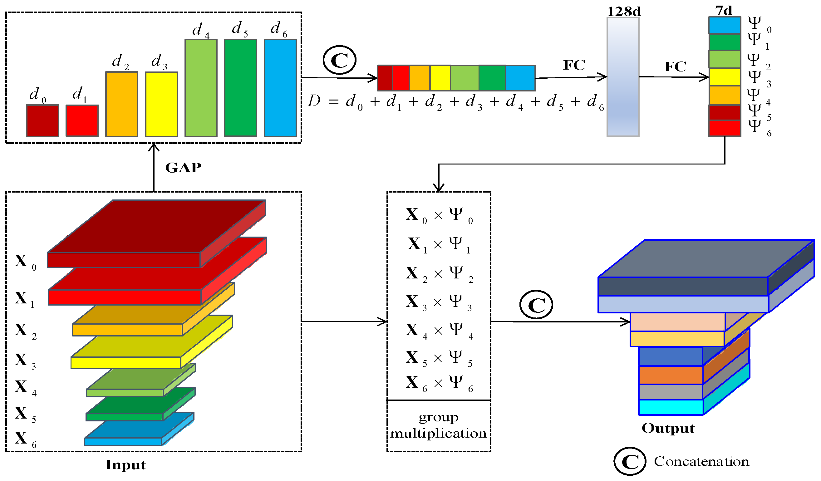
(1) We propose a multiscale feature aggregation network combining with a group-attention module (GAM) to reconstruct the quad-pol SAR data from the dual-pol SAR mode;
(2) The quad-pol SAR data reconstructed by our proposed method can sense changes in targets’ scattering mechanisms before and after a disaster;
(3) The quad-pol SAR data reconstructed by our proposed method achieve a 97.08% terrain classification accuracy, which is 1.25% higher than the dual-pol SAR data.
This paper is organized as follows: Section 2 introduces the proposed quad-pol SAR data reconstruction method. Section 3 analyzes the reconstructed quad-pol SAR data and its polarimetric target decomposition results. Section 4 compares the terrain classification results with real and reconstructed quad-pol SAR data. Section 5 discusses some issues in quad-pol SAR data reconstruction. Finally, conclusions are given in Section 6.

2. Quad-Pol SAR Data Reconstruction Method

2.1. Quad-Pol and Dual-Pol SAR Data Model

For polarimetric radar, the polarimetric scattering matrix with the basis of horizontal and vertical polarizations (H, V) can be expressed as
S = [ S HH S HV S VH S VV ]
where S VH means horizontal polarization transmitting and vertical polarization receiving, and other terms are similarly defined.
Under the reciprocity condition in polarimetric radar, the quad-pol SAR covariance matrix can be obtained as follows
C = [ | S HH | 2 2 S HH S HV * S HH S VV * 2 S HV S HH * 2 | S HV | 2 2 S HV S VV * S VV S HH * 2 S VV S HV * | S VV | 2 ]
where denotes the statistically average operation.
The normalized quad-pol SAR covariance matrix can be represented as
C P = [ δ 1 ρ 12 δ 1 δ 2 ρ 13 δ 1 δ 3 ρ 12 * δ 1 δ 2 δ 2 ρ 23 δ 2 δ 3 ρ 13 * δ 1 δ 3 ρ 23 * δ 2 δ 3 δ 3 ]
where P is the total backscattering power, which is defined as
P = | S HH | 2 + 2 | S HV | 2 + | S VV | 2
The other six parameters of the normalized covariance matrix are defined as follows
δ 1 = | S HH | 2 P , δ 2 = 2 | S HV | 2 P , δ 3 = | S VV | 2 P
ρ 12 = S HH S HV * | S HH | 2 | S HV | 2   ρ 13 = S HH S VV * | S HH | 2 | S VV | 2   ρ 23 = S HV S VV * | S HV | 2 | S VV | 2
Then, the normalized quad-pol SAR covariance matrix can be denoted as a vector
C f = [ δ 1 δ 2 δ 3 ρ 13 ρ 23 ρ 12 ] T
where the upper script T denotes the transpose operation. δ 1 , δ 2 , and δ 3 are real entities, while ρ 13 , ρ 23 , and ρ 12 are complex entities. Therefore, the normalized quad-pol SAR covariance matrix can be determined by nine real parameters.
In this paper, the HH and VH dual-pol SAR mode is considered without the loss of generality. However, other dual-pol SAR modes can be investigated in a similar manner. The dual-pol SAR covariance matrix is defined as a 2 × 2 matrix that represents the polarimetric information of the radar image. In the case of the HH and VH polarization channels, the dual-pol SAR covariance matrix is given as follows:
C dual = [ | S HH | 2 S HH S HV * S HV S HH * | S HV | 2 ]

2.2. Quad-Pol SAR Data Reconstruction from the Dual-Pol SAR Mode

The quad-pol SAR is able to provide complete polarization information, but it is limited by its narrow observation swath and system complexity. On the other hand, the dual-pol SAR has a wider swath but lacks partial polarization information. The reconstruction of the quad-pol SAR covariance matrix mainly utilizes two sources of information. Firstly, the contextual information of the dual-pol SAR images can be employed to reconstruct the remaining polarization channels. Therefore, multiscale spatial features extracted by convolutional layers can be utilized for the quad-pol SAR data reconstruction. Secondly, as Formula (3) reveals, the elements of the quad-pol SAR covariance matrix are determined by several parameters together, which indicates that there is a certain relationship between different polarization channels for specific land covers. With the help of deep CNN models, we can establish a mapping relationship between the dual-pol SAR data and quad-pol SAR covariance matrix. Once the quad-pol SAR data are reconstructed, well-established, fully polarimetric techniques can be applied to dual-pol SAR image processing. This opens up many interesting applications based on quad-pol SAR images that can be extended into dual-pol SAR data, and its performance is expected to be correspondingly improved.
To achieve this goal, in this paper, we propose a dual-pol to quad-pol network (D2QNet) to reconstruct the quad-pol SAR image from the dual-pol SAR data. As illustrated in Figure 1, the D2QNet-v2 architecture consists of two parts: the feature extraction (FE) network and the feature translation (FT) network. The FE network extracts features in both spatial and polarimetric domains and encodes them into a compact feature representation, while the FT network decodes this representation and generates the quad-pol SAR covariance matrices. It should be further pointed out that the only difference between the D2QNet-v1 and D2QNet-v2 is the absence of the GAM in the FE network for the D2QNet-v1.
In the D2QNet-v2 model, the FE network is composed of the first seven convolutional layers of the VGG16 network, as well as a group attention module (GAM), feature map interpolation, and normalization operations. The detailed configuration of part of the VGG16 network is provided in Table 1, which consists of seven convolutional layers with a kernel size of 3 × 3, a rectified linear unit (ReLU) activation function, and a max-pooling layer. To reduce the number of network parameters and prevent overfitting, pretrained weights from the ImageNet dataset [17] are utilized in the FE network. However, since the dual-pol SAR images have four channels, unlike the optical images that the VGG16 network was initially designed for, the first layer of the FE network is adapted to accommodate all four input channels. Specifically, the first three channels’ weights are identical to the first layer of the pretrained VGG16 network, and the weights of the fourth channel are calculated by taking the average of the weights of the first three channels.
The input dual-pol SAR data can be represented as
X = [ | S HH | 2 | S HV | 2 Re [ S HV S HH * ] Im [ S HV S HH * ] ]
where subscript k denotes the k-th SAR image; Re [ ] and Im [ ] are to obtain the real and imaginary part of the complex number, respectively.
The multiscale feature groups extracted from the dual-pol SAR data by the different layers of the FE network are denoted as X n , n { 0 , 1 , 2 , 3 , 4 , 5 , 6 } , with each group having a channel number of d n { 64 , 64 , 128 , 128 , 256 , 256 , 256 } . These multiscale feature groups are then passed through the GAM, which efficiently aggregates and fuses the multiscale features from the different layers into feature maps that have access to both high- and low-level information [34]. As shown in Figure 2, the GAM firstly applies global average pooling (GAP) to each feature group, squeezing their spatial information. Then, it concatenates channel-wise statistical information from all groups to integrate intergroup and outergroup contexts, forming a global feature representation. Specifically, given each feature group X n H n × W n × d n , the GAM calculates the channel-wise global representation as
Y = concat { 1 H n × W n i = 1 H n j = 1 W n X n ( i , j ) }
where concat { } is the concatenation operation, D = n = 1 N d n is the channel number of global representation Y , N stands for the number of feature groups, and ( i , j ) is the spatial coordinate of feature map.
To progressively fuse the multiscale features, two fully connected (FC) layers are used to learn the attention maps Ψ that weight different feature groups. These attention maps can be denoted as
Ψ = W 2 ( ReLU ( W 1 ( Y ) ) )
where W 1 and W 2 are the network weights of two FC layers. The dimensions of the two FC layers are set to 128 and 7, respectively.
Finally, each original feature group is enhanced by multiplying the channel-wise global representation of each feature group X n with the corresponding weights in the attention map Ψ n , and the importance of each feature group is weighted as
X ˜ n = X n Ψ n
where Ψ n is the n-th element of Ψ and means element-wise multiplication between X n and Ψ n .
Therefore, the GAM enables the D2QNet-v2 model to selectively focus on the most informative and discriminative feature groups at each step of the fusion process.
The enhanced feature maps are interpolated to the same size as the input dual-pol SAR images X and then are concatenated together to form a high-dimensional feature representation F as
F = concat { X , X ˜ 0 , X ˜ 1 , UP ( X ˜ 2 ) , UP ( X ˜ 3 ) , UP ( X ˜ 4 ) , UP ( X ˜ 5 ) , UP ( X ˜ 6 ) }
where UP ( ) denotes the upsampling operation with a bilinear interpolation.
This feature representation captures both low-level and high-level information extracted from different scales of the dual-pol SAR data. In order to ensure the feature maps in F are all on the same scale and have consistent ranges, the feature representation F is normalized as follows
F ˜ l F l μ l σ l , l = 1 , 2 , 3 , , 7
where F l is the l-th feature maps, while μ l and σ l are the mean and variance values of F l .
Finally, the normalized compact feature representation F ˜ l is fed into the FT network for guiding the quad-pol SAR data reconstruction.
The FT network is proposed to map the compact feature representation F ˜ l into the polarimetric covariance matrix, which is made up of three 1 × 1 convolutional layers with depths of 512, 256, and 32. The module names and corresponding parameters of the FT network are given in Table 2. It can be seen that each convolutional layer is followed by a ReLU activation function. The nine real elements of the normalized covariance matrix C f are quantified into thirty-two quantization levels, and the softmax function after the last convolutional layer is utilized to predict the quantization levels of the nine real elements. The use of 1 × 1 convolutional kernels allows for the efficient fusion of different feature maps, which is more efficient than the fully connected networks proposed in [30] for generating SAR images pixel-by-pixel.
The cross-entropy loss function is adopted to drive the network.
L o s s _ r e c = 1 9 Q j = 1 9 q = 1 Q δ [ y i ( j ) = q ] In [ p i ( j ) ( q ) ]
where Q is the number of quantize levels to be classified and Q = 32. y i ( j ) is the truth value of the j-th parameter of the i-th pixel. p i ( j ) ( q ) is the probability of the j-th parameter of the i-th pixel being in the q-th center quantization value. δ ( ) is the indication function and its value equals 1 if y i ( j ) = q and 0 otherwise. In ( ) is the natural logarithm function.
Once the nine real parameters of the normalized quad-pol SAR covariance matrix are reconstructed, the total backscattering power and other elements of the quad-pol SAR covariance matrix can be calculated as follows
P = | S HH | 2 δ 1 ,   | S VV | 2 = P δ 3
S HH S VV * = ρ 13 | S HH | 2 P δ 3 ,   S HV S VV * = ρ 23 | S HV | 2 P δ 3

3. Experimental Evaluation with Model-Based Decomposition

Multitemporal ALOS/PALSAR PolSAR datasets from the March 11 East Japan earthquake and tsunami, which caused extensive damage to coastal buildings, are adopted for subsequent quad-pol SAR data reconstruction performance analysis. The pre-event dataset was acquired on 21 November 2010, and the post-event dataset was obtained on 8 April 2011.
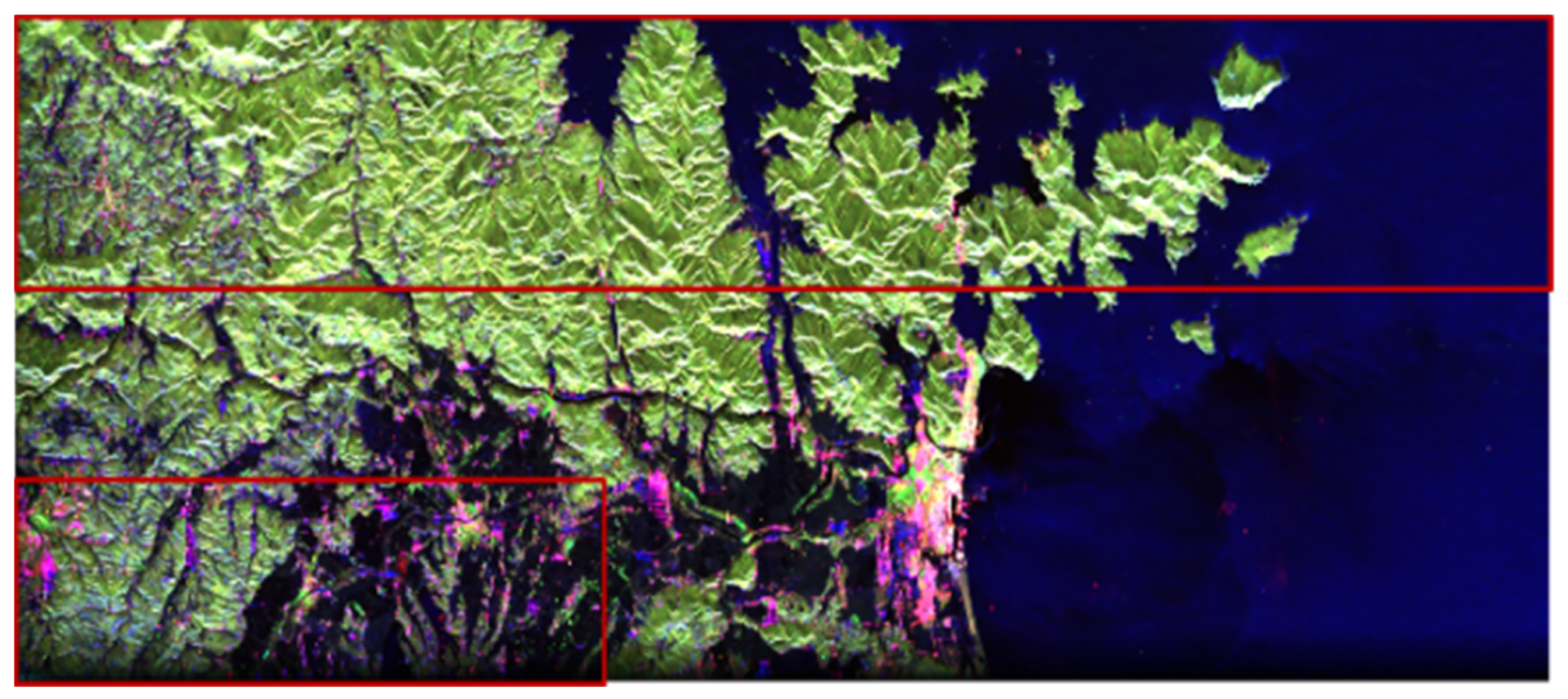
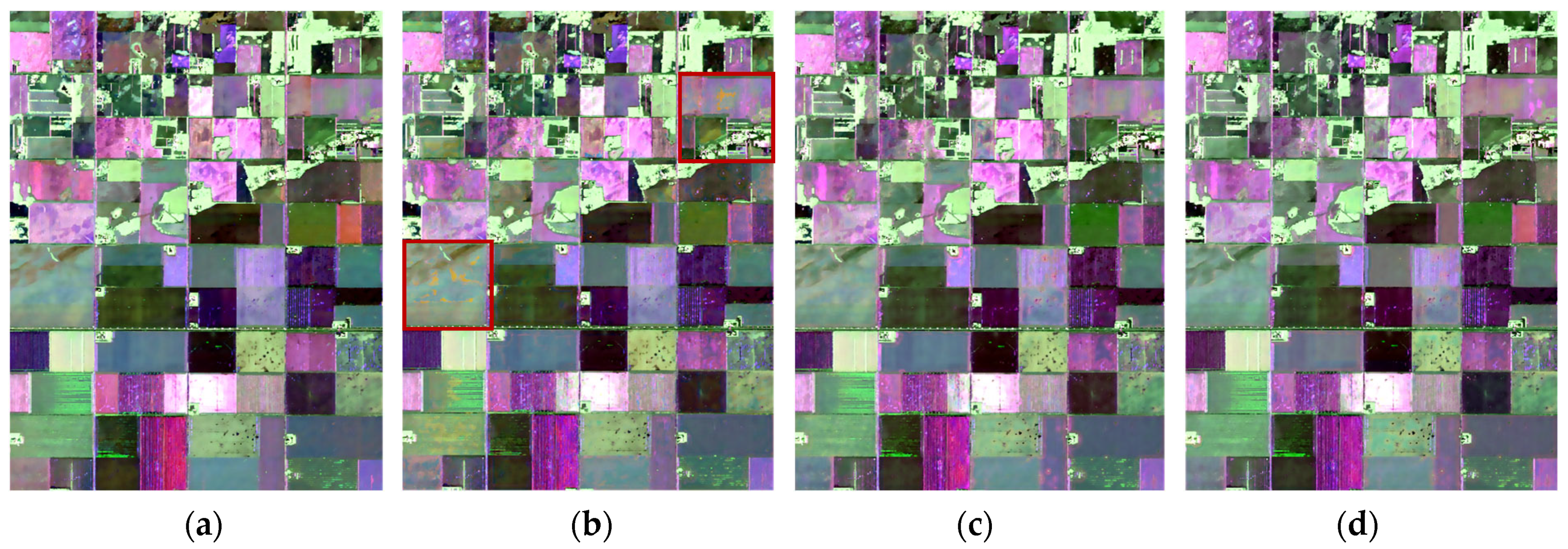
The HH and VH dual-pol SAR data are simulated from original PolSAR datasets for subsequent investigation. The training datasets are selected from the post-event data, which are circled in a red rectangle, as shown in Figure 3. Total pixels in the training datasets account for 52.16% of the whole SAR image. The remaining post-event data and all pre-event data are used to construct the testing datasets. In order to train the network without taking up too much memory, the whole SAR image is cut into 400 × 400 slice images with a 25% overlapping rate. To the best of our knowledge, quad-pol SAR data reconstruction from dual-pol SAR data has not been reported. The DNN method in [19] can reconstruct quad-pol SAR data from single-polarization SAR data, which is chosen as the comparison algorithm. The first layer of the DNN method is similarly adjusted to four channels to adapt the dimension of the dual-pol SAR data.
The random gradient descent method (Adam optimizer) is utilized to train the network, and its parameters are set as follows: β 1 = 0.9 , β 2 = 0.999 , ε = 10 6 , and the learning rate is 0.0001. The network is trained to converge until the number of epochs reaches 100.

3.1. Quantitative Reconstruction Performance Evaluation
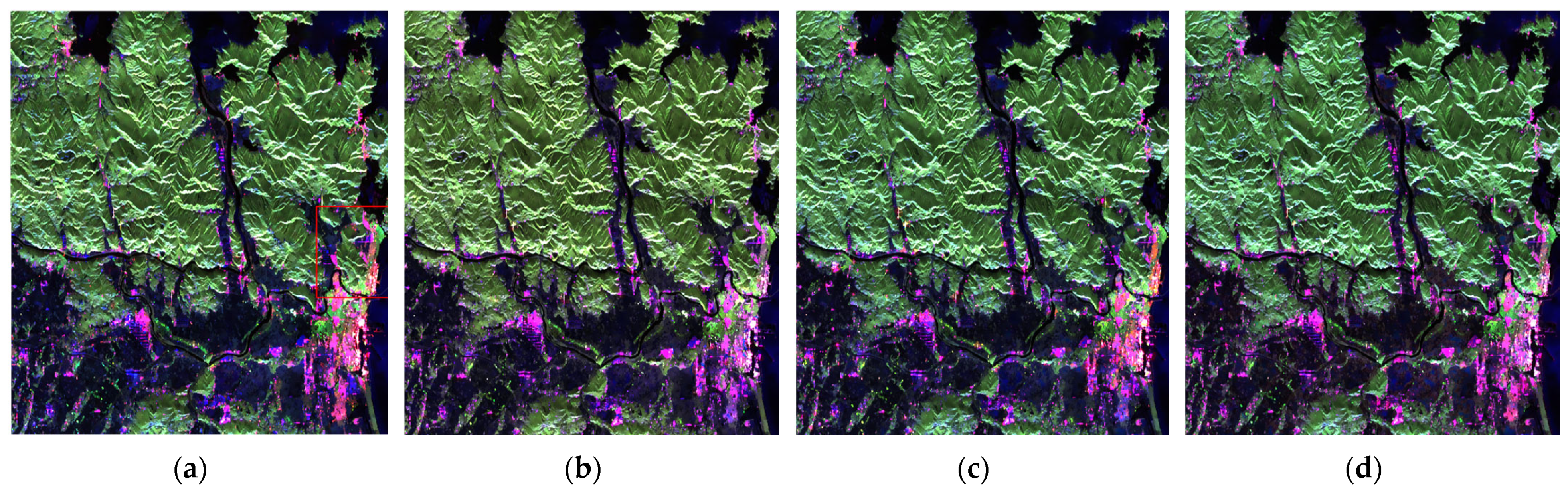
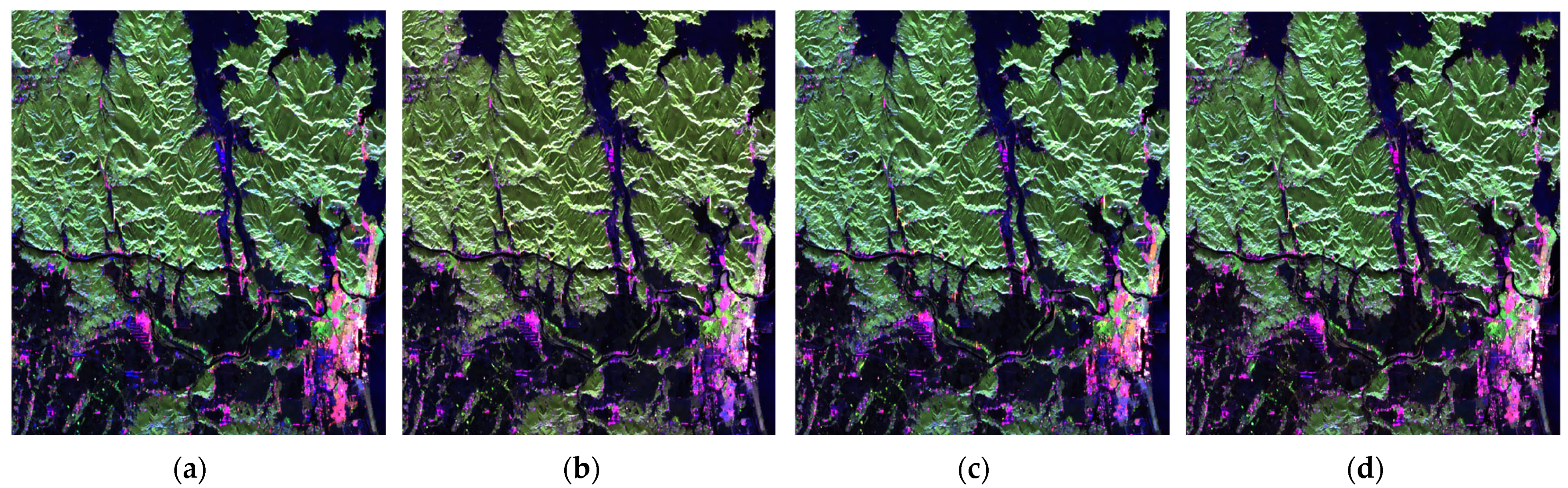
As shown in Figure 4, the pre-event Pauli images obtained by different reconstruction methods and the real quad-pol SAR data are compared. Visually, the pre-event Pauli images reconstructed by the proposed D2QNet-v1 and D2QNet-v2 methods are mostly identical to the real quad-pol SAR case. However, the Pauli image obtained by the DNN method shows larger differences in forest areas and seashore buildings when compared to the real quad-pol SAR data.
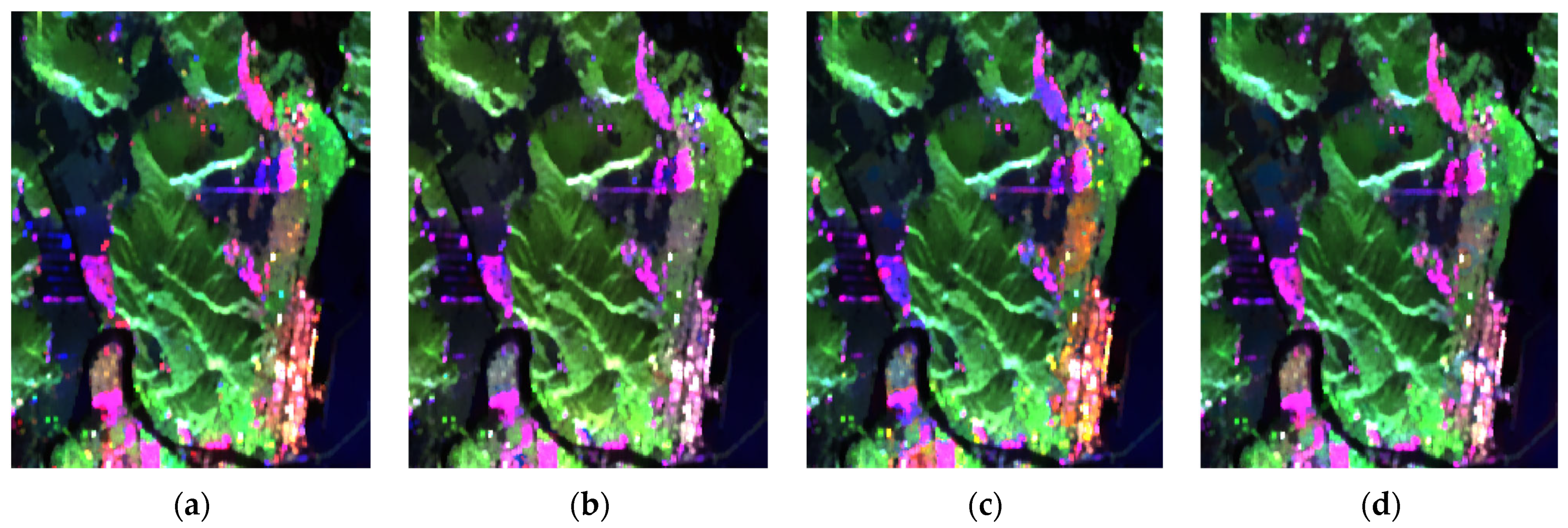
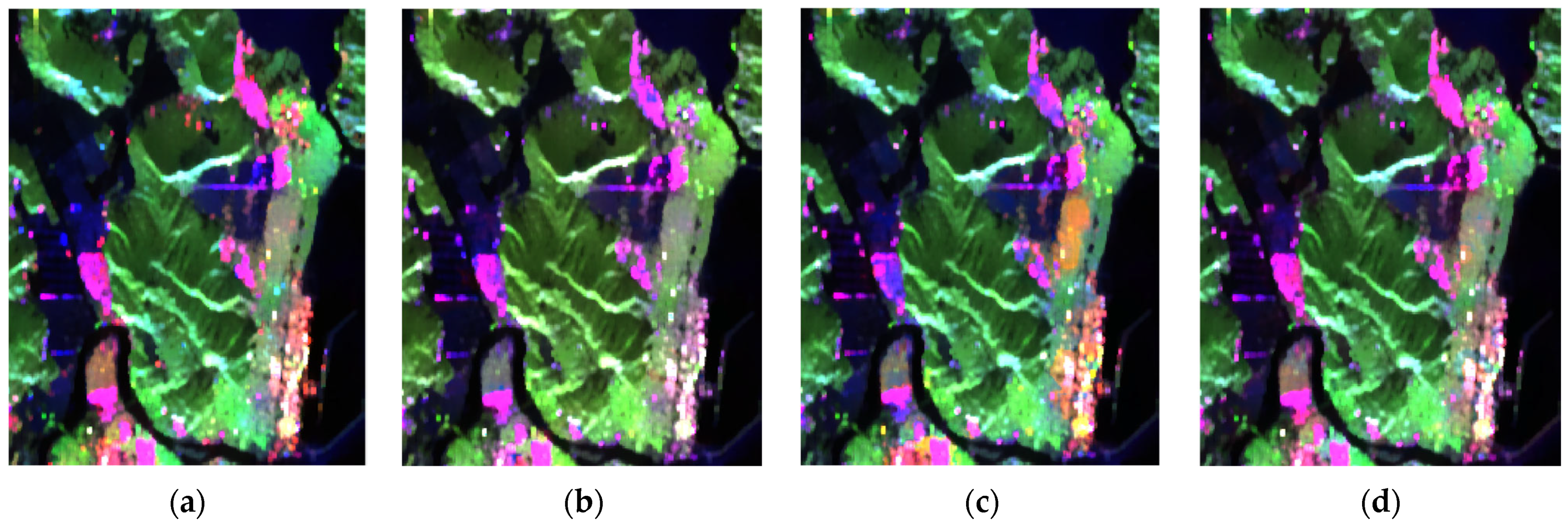
To validate the excellent performance of the proposed methods, we further analyze severely damaged Ishinomaki city, circled in a red rectangle window in Figure 4a. The pre-event Pauli images of Ishinomaki city are shown in Figure 5. It can be seen that the proposed D2QNet-v1 method achieves better visual performance in the coastal-building area than the DNN method. Although the D2QNet-v2 method has some deficiencies in reconstructing the scattering information of coastal buildings, it can remove some artifacts of the D2QNet-v1 method and obtain preferable results in the whole Pauli images. Nevertheless, the quad-pol SAR data reconstructed by the DNN method is not effective over buildings and forest areas. Note that, since the FT network in the DNN method only adopts a fully connected network that is unable to capture spatial correlation information among pixels, its reconstruction performance is correspondingly decreased.
To further verify the advantages of the proposed D2QNet-v1 and D2QNet-v2 methods, the coherence index (COI) and mean absolute error index (MAE) are utilized to evaluate the accuracy of the reconstructed polarimetric channels.
COI ( A , B ) = i = 1 M j = 1 N A i j B i j * i = 1 M j = 1 N A i j A i j * × i = 1 M j = 1 N B i j B i j *
MAE ( A , B ) = 1 M N i = 1 M j = 1 N | A i j B i j |
where M and N represent the number of rows and columns of the matrix A and B , respectively.
As shown in Table 3 and Table 4, the COI and MAE results of the reconstructed quad-pol SAR data in the pre-event indicate that the proposed D2QNet-v1 and D2QNet-v2 methods have higher COI values and a lower reconstruction error in nearly all reconstructed polarimetric channels than the DNN method. The COI value of Im( C 13 ) of the DNN method is negative, which means that its reconstruction appears with serious problems. It is worth noting that the COI and MAE indexes in one polarimetric channel cannot always reflect the advantages of the reconstruction methods, and the COI is not strictly consistent with the MAE index. In other words, higher COI values do not necessarily mean that the overall reconstruction error is lower. Detailed reasons for this are explained in the Discussion section.
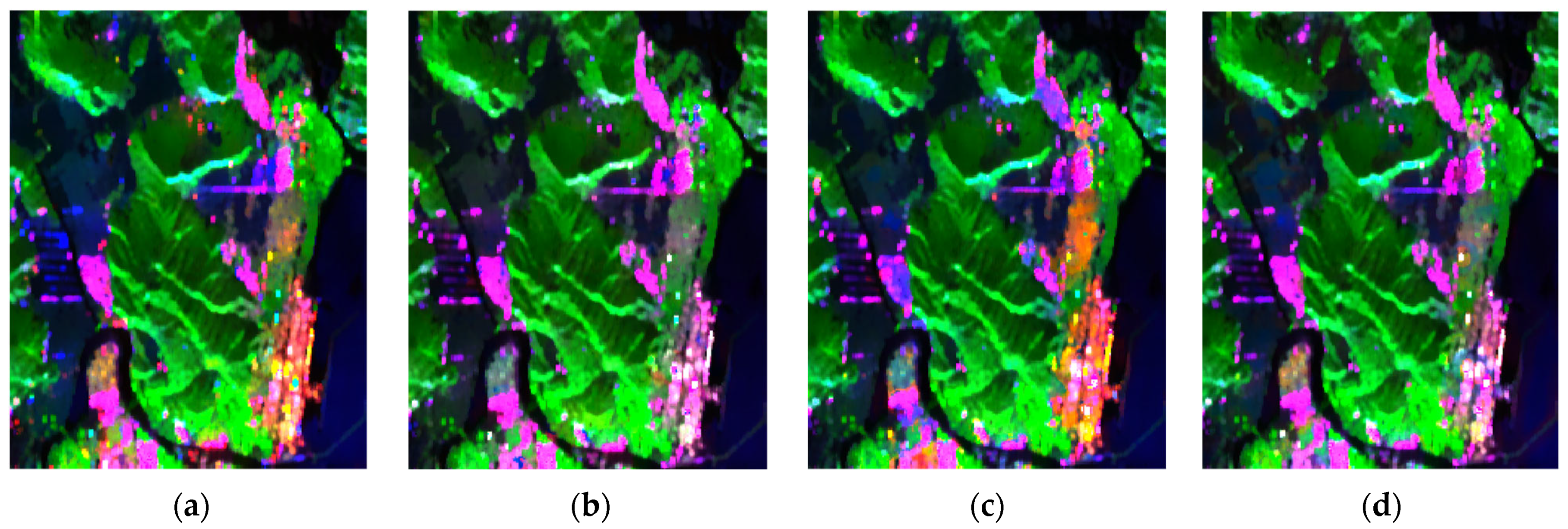
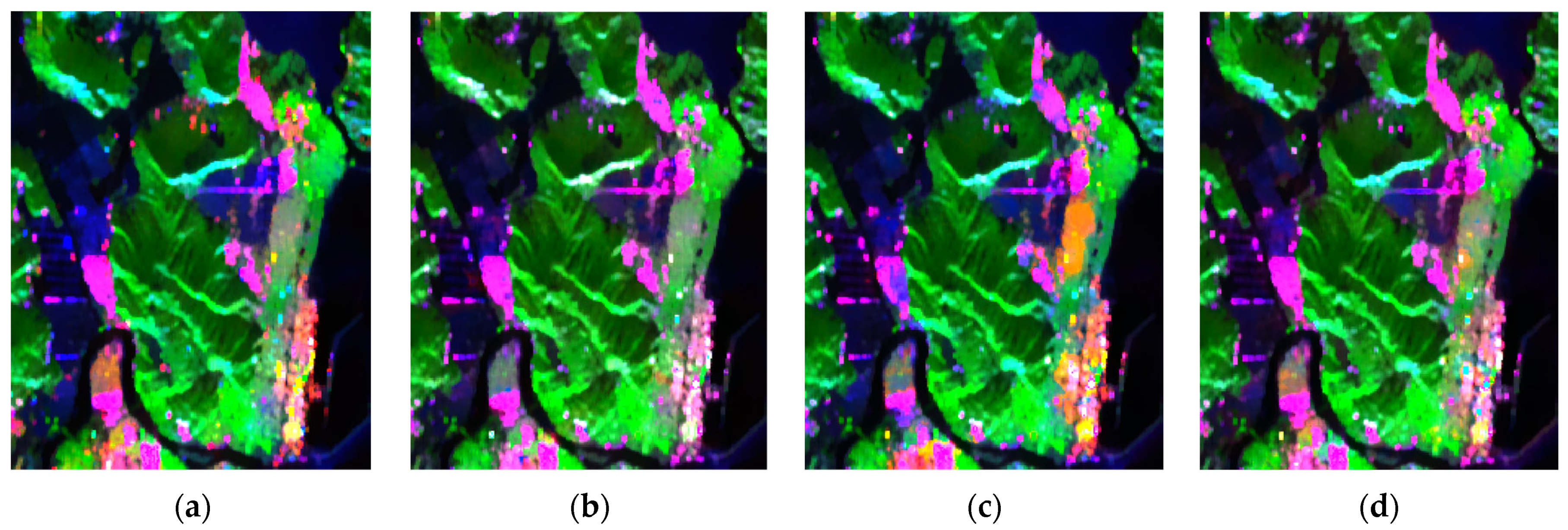
The post-event Pauli images of the real quad-pol SAR data and the different reconstruction methods are shown in Figure 6, and their Pauli images of Ishinomaki city are shown in Figure 7. Overall, it can be seen that the proposed D2QNet-v2 method achieves the best visual performance among all reconstruction methods. The D2QNet-v1 method provides a preferable visual experience in coastal-building areas. However, in forest and other complex regions, the DNN method produces biased reconstruction results.
Quantitative comparison results in terms of the COI and MAE indexes are given in Table 5 and Table 6. Similar to the pre-event case, the proposed D2QNet-v1 and D2QNet-v2 methods achieve a superior performance to the DNN method. The polarimetric channel Im( C 13 ) reconstructed by the DNN method is also negatively correlated with the real quad-pol SAR data. From a reconstruction error perspective, the proposed D2QNet-v2 method obtained optimal quantitative comparison results.

3.2. Quantitative Comparison with Model-Based Target Decomposition

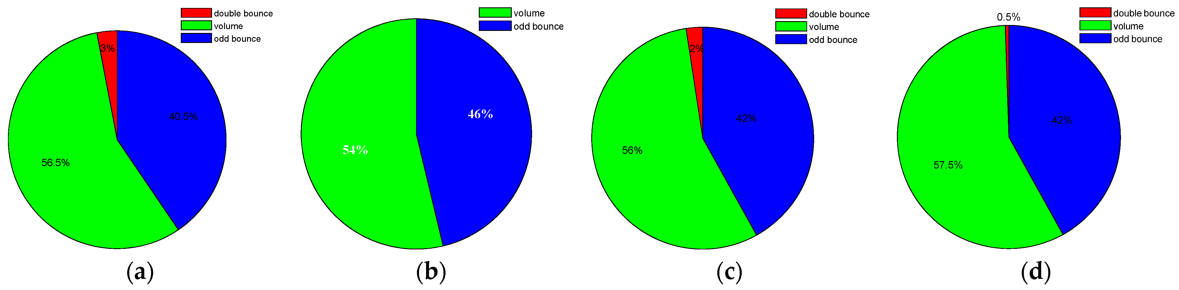
In order to evaluate the reconstruction performance more effectively, we utilize polarimetric target decomposition to assess the scattering mechanism preservation between the real and reconstructed quad-pol data. Specifically, we use the Yamaguchi target decomposition method on real and reconstructed quad-pol data, and the decomposed results are illustrated in Figure 8. The red, green, and blue color of the Pauli images represent the double-bounce scattering, volume scattering, and odd-bounce scattering, respectively. Figure 9 shows the proportions of double-bounce, odd-bounce, and volume-scattering components in Figure 8. It can be seen that the quad-pol SAR data reconstructed by the proposed D2QNet-v1 method has the best scattering mechanism reconstruction performance, with a scattering mechanism that is consistently similar to that of the real quad-pol SAR data. However, the DNN method seriously underestimates the double-bounce-scattering component, causing its value to become zero. Additionally, the DNN method overestimates the odd-bounce scattering and underestimates the volume scattering, leading to poor reconstruction performance in forest areas. It should be noted that the targets’ scattering information reconstructed by the DNN method is completely out of line with the real quad-pol SAR data, rendering it unusable for practical applications.
Similar to the pre-event case, the Yamaguchi target decomposition results of the real and reconstructed quad-pol data in the post-event are displayed in Figure 10. Figure 11 shows the proportions of the double-bounce, odd-bounce and volume-scattering components in Figure 10. Compared with the real quad-pol SAR data, the quad-pol SAR data reconstructed by the proposed D2QNet-v1 method outperforms other methods in terms of preserving the scattering mechanism. In Ishinomaki city, which suffered severe damage in the post-event, a large number of buildings collapsed and the corresponding double-bounce-scattering component was reduced. As a result, the percentage of double-bounce-scattering components obtained by the proposed D2QNet-v1 method has decreased by 2%, which is consistent with the real quad-pol SAR case. It should be noted that obtaining accurate information on double-bounce scattering changes is critical for disaster evaluation. However, the DNN method still overestimates the odd-bounce scattering and underestimates the volume and double-bounce scattering, which renders the quad-pol SAR data reconstructed by the DNN method ineffective for practical applications.
In summary, compared with the DNN method, the proposed methods achieve superior qualitative and quantitative quad-pol SAR data reconstruction performance. Moreover, the proposed method can preserve the targets’ scattering mechanism well, further confirming its excellent reconstruction performance.

4. Experimental Evaluation with Terrain Classification

4.1. Quantitative Reconstruction Performance Evaluation

Multitemporal PolSAR data have become increasingly important for applications such as terrain classification and growth monitoring. In this section, we adopt the NASA/JPL UAVSAR airborne L-band PolSAR data over Southern Manitoba, Canada, for further analysis [7]. The pixel resolutions are 5 m and 7 m in range and azimuth directions, respectively. The selected region for investigation comprises seven crop types, including corn, wheat, broadleaf, forage crops, soybeans, rapeseed, and oats. These multitemporal PolSAR images have been coregistered and their size is 1300 × 1000. The training and testing data were collected on June 22nd (0622) and June 23rd (0623), respectively. Figure 12 shows the PolSAR Pauli image of the training data and the corresponding ground-truth image.
The UAVSAR 0623 Pauli images of the real quad-pol SAR data and different reconstruction methods are shown in Figure 13. The reconstructed Pauli images have a high degree of visual similarity to the real quad-pol SAR case, although differences can be observed between the different reconstruction methods. It should be further pointed out that some reconstruction artifacts appear in the DNN method, circled in a red rectangle frame in Figure 13b. These artifacts are likely caused by the limitations of the fully connected layers in the feature translation network used in the DNN method. This phenomenon is similar with the results presented in the previous section.
The COI and MAE results of the different reconstructed quad-pol SAR data are shown in Table 7 and Table 8. Although the DNN method obtains better quantitative COI and MAE values in some polarimetric channels, the COI value of Re( C 13 ) of the DNN method is −0.8816. This indicates that the DNN method may have limitations in accurately reconstructing certain polarimetric features. In addition, the proposed D2QNet-v1 and D2QNet-v2 methods have their respective reconstruction advantages in certain polarimetric channels. Therefore, it is difficult to identify which reconstruction method is the best based solely on COI and MAE indicators. A more comprehensive evaluation approach is to apply the reconstructed quad-pol SAR data to terrain classification to validate its advantages in this section.

4.2. Classification Method

In Section 2, the quad-pol SAR covariance matrices C of the whole SAR images are reconstructed from the dual-pol SAR data. Then, the corresponding polarimetric coherency matrices T 3 can be obtained. To validate the reconstruction effectiveness of the proposed method, terrain classification is carried out based on the reconstructed quad-pol SAR coherency matrices T 3 . Instead of directly using the elements of the coherency matrices T 3 for terrain classification, polarimetric features are extract from T 3 based on polarimetric target decomposition. Inspired by SFCNN [7], three roll-invariant polarimetric features and two hidden polarimetric features in the rotation domain, extended to the reconstructed quad-pol SAR data, are selected for terrain classification.
The selected roll-invariant polarimetric features contain total backscattering power P , entropy H , mean alpha angle α ¯ , and anisotropy A n i .
According to the eigenvalue decomposition theory [26], the quad-pol SAR coherency matrix T 3 can be decomposed as
T 3 = U [ λ 1 0 0 0 λ 2 0 0 0 λ 3 ] U H , λ 1 λ 2 λ 3
where λ 1 , λ 2 , and λ 3 are the eigenvalues, while U contains the decomposed eigenvectors.
The polarimetric entropy H , mean alpha angle α ¯ , and anisotropy A n i features can be derived from the decomposed eigenvalues λ i , as follows
H = i = 1 3 p i log p i , α ¯ = i = 1 3 p i α i , A n i = λ 2 λ 3 λ 3 + λ 3
where p i = λ i / ( λ 1 + λ 2 + λ 3 ) .
In [7,29], two null angle features in the rotation domain are developed, which are sensitive to various land covers. Their definitions can be formulated as
θ null _ Re [ T 12 ] = 1 2 Angle { Re [ T 13 ] + j Re [ T 12 ] } = 1 2 Angle { Re [ ( S HH + S VV ) S HV * ] + j 1 2 ( | S VV | 2 | S HH | 2 ) }
θ null _ Re [ T 12 ] = 1 2 Angle { Im [ T 13 ] + j Im [ T 12 ] } = 1 2 Angle { Im [ ( S HH + S VV ) S HV * ] + j Im [ S HH S VV * ] }
where Angle { } is the operator to obtain the phase of a complex value within the range of [ π , π ] .
After the extraction of the six polarimetric features, a simple CNN model is adopted for terrain classification [7]. The architecture of the CNN model is shown in Figure 14. The size of the input patches is set to 13 × 13 × d, where d represents the number of polarimetric features. The CNN model consists of three convolutional layers, two max pooling layers, two fully connected (FC) layers, and a softmax layer. The cross-entropy loss function is utilized to drive the CNN classifier.
In summary, the terrain classification method is summarized as follows:
(a)
Apply speckle filtering to the quad-pol SAR images to reduce speckles [35,36,37];
(b)
Construct patches from the quad-pol SAR images by using a sliding 13 × 13 window;
(c)
Extract polarimetric features from each pixel;
(d)
Select a percentage of the labeled samples randomly as training datasets to train the CNN classifier. The remaining labeled samples are used as testing datasets;
(e)
Classify the testing datasets based on the trained CNN classifier and evaluate its classification accuracy.

4.3. Quantitative Comparison

Five terrain-classification experiments are conducted to evaluate the efficacy of the proposed reconstruction methods. The input data for the CNN model includes: (i) dual-pol SAR data, six selected polarimetric features directly extracted from (ii) real quad-pol SAR data, (iii) quad-pol SAR data reconstructed by the DNN method, (iv) quad-pol SAR data reconstructed by the D2QNet-v1 method, and (v) quad-pol SAR data reconstructed by the D2QNet-v2 method. The training rate is set to 1%. In order to choose the optimal training model, the training and verification datasets are divided into a ratio of 8:2 in the training datasets. The remaining pixels are used as testing datasets.
The stochastic gradient descent (SGD) optimizer is employed to train the network, and the momentum is set to 0.9. The learning rate is 0.001 and the number of training epoch is set to 200.
The terrain classification results of the UAVSAR 0623 images are shown in Figure 15 and the classification accuracies of different methods are given in Table 9. Undoubtedly, the real quad-pol SAR data achieve the highest classification accuracy of 98.03%. Compared with dual-pol SAR data, the quad-pol SAR data reconstructed by the DNN method and the proposed D2QNet-v1 method have a lower classification accuracy. Even so, the proposed D2QNet-v1 method has a higher accuracy than the DNN method. As can be seen in Figure 15, the classification results of the proposed D2QNet-v2 method have the minimum number of error classification pixels than other methods, especially in rapeseed and wheat classes. In detail, the confusion matrix of the proposed D2QNet-v2 method and its classification accuracies for each terrain class are given in Table 10. The rows represent the real terrain types, while the columns represent the predicted terrain types. The values in each cell represent the number of samples that were classified as a particular terrain type. It is worth noting that the proposed D2QNet-v2 method achieves a 1.25% accuracy improvement compared to the dual-pol SAR case, and is only 0.95% lower than the real quad-pol SAR case. The classification accuracies of the proposed D2QNet-v2 method for all terrain classes are over 95% except for rapeseed class.
To sum up, the proposed D2QNet-v2 method utilizes the GAM to obtain abundant semantic information and aggregate the multiscale features effectively. Compared with the DNN method, the quad-pol SAR data reconstructed by the proposed D2QNet-v2 method can achieve a superior terrain classification performance.

5. Discussion

5.1. One-Sidedness of COI and MAE Indexes

In this section, we combine the visualization analysis in two-dimensional space to illustrate the limitations of using COI and MAE indexes to evaluate the reconstruction performance. As shown in Figure 16, the real quad-pol SAR data are annotated as a blue point, and a blue circle is drawn with this point as the center. Except for the blue point, other points in two-dimensional space represent the reconstructed quad-pol SAR data. According to Formulas (18) and (19), COI can be interpreted as the cosine of the angle between two lines and the MAE index can be considered as the distance between two points. It is observed that all points on the blue circle have the same MAE index values. However, the COI values of these points on the blue circle have different COI values. Compared with lines l1 and l2, the COI of the points in line l4 have higher values, but not all the points in line l4 have lower MAE values. In addition, the values of the MAE index decrease as the radius of the blue circle shrinks, but their corresponding COI values are not always increasing. It is worth noting that the COI values of the intersection points between the blue circle and line l3 always remain at one, regardless of the size of the blue circle. However, the values of the MAE index increase when the blue circle enlarges. For line l5, the COI values become negative, which is the same case as the DNN method in reconstructing some polarimetric channels.
Therefore, we can conclude that simply using COI and MAE indexes in one polarimetric channel cannot reflect the advantages of the reconstruction method. The evaluation methods should focus on applying the reconstructed quad-pol SAR data to improve the performance of subsequent tasks, such as terrain classification or target detection.

5.2. Limitations of Quad-Pol SAR Data Reconstruction Methods

Although reconstructing the quad-pol SAR data from the dual-pol SAR mode has many advantages, it also brings the following issues. Firstly, it is common to perform multilook processing on SAR images before reconstructing the quad-pol data to ensure the full-rank property of the quad-pol SAR covariance matrix. This preprocessing step may indeed reduce the spatial resolution of the SAR image. Secondly, as a special form of the dual-pol SAR mode, reconstructing the quad-pol SAR data from the compact-polarization mode requires the assumption of reflection symmetry. Additionally, the polarization interpolation model is used to estimate the cross-polarization terms, which results in a certain level of error between the reconstructed quad-pol SAR data and the real quad-pol SAR data. The lack of generalizability often appears when reconstructing quad-pol SAR data with networks. In future work, physical characteristics will be fused into the network architecture design to improve the interpretability and generalizability of the network models.

5.3. Comparison of Training Time

Compared to the DNN method that uses a fully connected network for pixel-by-pixel reconstruction, the proposed methods utilize a fully convolutional network to achieve quad-pol SAR data reconstruction for the whole image. As shown in Table 11, the proposed D2QNet-v1 and D2Qnet-v2 methods offer a faster training speed than the DNN method. Due to the addition of the GAM, the training speed of the D2QNet-v2 method is slightly slower than the D2QNet-v1 method.

6. Conclusions

In this work, a novel multiscale feature aggregation network is proposed to reconstruct the quad-pol SAR data from the dual-pol SAR mode. The core idea is extending well-established full-polarimetric techniques to the dual-pol SAR mode and improving the terrain-classification performance of the dual-pol SAR data. Firstly, multiscale features are extracted from the pretrained VGG16 network. Then, a group-attention module is designed to enhance the multiscale feature maps and fuse the high- and low-level information of multiple layers. Finally, the original dual-pol SAR images and fused feature maps are concatenated and mapped into polarimetric covariance matrices through a full convolutional neural network. Comparative experimental studies are conducted on different bands and sensors of the SAR datasets from ALOS/PALSAR and UAVSAR, and the proposed methods exhibit higher COI and lower MAE indicators. Furthermore, the results of the Yamaguchi target decomposition on the reconstructed quad-pol SAR data indicate that the proposed method can better preserve targets’ scattering information. Compared with the dual-pol SAR data, the reconstructed quad-pol SAR data of the proposed D2QNet-v2 method can achieve a 97.08% terrain classification accuracy and an improvement of 1.25% over the dual-pol SAR data. From the perspective of training-network effectiveness, the proposed methods require less training time than the DNN method. Future work will focus on comparing the reconstructed quad-pol SAR data with dual-pol SAR data on the performance of ship detection.

Author Contributions

J.D., S.C. and P.Z. provided ideas; J.D. and P.Z. validated the idea and established the algorithm; J.D., P.Z., M.L. and S.C. designed the experiment; J.D., H.L. and S.C. analyzed the results of the experiment; J.D., M.L. and H.L. wrote the paper. All authors have read and agreed to the published version of the manuscript.

Funding

This research was funded in part by the National Natural Science Foundation of China, 62122091 and 61771490, the Research Foundation of Satellite Information Intelligent Processing and Application Research Laboratory, and the Natural Science Foundation of Hunan Province under grant 2020JJ2034.

Institutional Review Board Statement

Not applicable.

Informed Consent Statement

Not applicable.

Data Availability Statement

The datasets used and/or analyzed during the current study are available from the corresponding author on reasonable request.

Acknowledgments

The authors would also like to thank the editors and anonymous reviewers for their constructive suggestions, which greatly contributed to improving this paper.

Conflicts of Interest

The authors declare no conflict of interest.

References

  1. Cumming, G.; Wong, H. Digital Processing of Synthetic Aperture RADAR Data; Artech House: Boston, MA, USA, 2005; pp. 108–110. [Google Scholar]
  2. Lee, S.; Pottier, E. Polarimetric Radar Imaging: From Basics to Applications; CRC Press: Boca Raton, FL, USA, 2009. [Google Scholar]
  3. Chen, S.; Wang, X.; Xiao, S.; Sato, M. Target Scattering Mechanism in Polarimetric Synthetic Aperture Radar-Interpretation and Application; Springer: Singapore, 2018. [Google Scholar]
  4. Sato, M.; Chen, S.; Satake, M. Polarimetric SAR Analysis of Tsunami Damage Following the 11 March 2011 East Japan Earthquake. Proc. IEEE 2012, 100, 2861–2875. [Google Scholar] [CrossRef]
  5. Chen, S.; Sato, M. Tsunami Damage Investigation of Built-Up Areas Using Multitemporal Spaceborne Full Polarimetric SAR Images. IEEE Trans. Geosci. Remote Sens. 2013, 51, 1985–1997. [Google Scholar] [CrossRef]
  6. Tao, C.; Chen, S.; Li, Y.; Xiao, S. PolSAR Land Cover Classification Based on Roll-Invariant and Selected Hidden Polarimetric Features in the Rotation Domain. Remote Sens. 2017, 9, 660. [Google Scholar] [CrossRef]
  7. Chen, S.; Tao, C. PolSAR Image Classification Using Polarimetric-Feature-Driven Deep Convolutional Neural Network. IEEE Geosci. Remote Sens. Lett. 2018, 9, 660–664. [Google Scholar] [CrossRef]
  8. Chen, S.W.; Tao, C.S. Multi-temporal PolSAR crops classification using polarimetric-feature-driven deep convolutional neural network. In Proceedings of the 2017 International Workshop on Remote Sensing with Intelligent Processing (RSIP), Shanghai, China, 18–21 May 2017; pp. 1–4. [Google Scholar]
  9. Deng, J.; Li, H.; Cui, X.; Chen, S. Multi-Temporal PolSAR Image Classification Based on Polarimetric Scattering Tensor Eigenvalue Decomposition and Deep CNN Model. In Proceedings of the IEEE International Conference on Signal Processing, Communications and Computing, Xi’an, China, 25–27 October 2022; pp. 1–6. [Google Scholar]
  10. Ainsworth, T.L.; Preiss, M.; Stacy, N.; Lee, J.S. Quad polarimetry and interferometry from repeat-pass dual-polarimetric SAR imagery. In Proceedings of the IEEE International Geoscience and Remote Sensing Symposium, Barcelona, Spain, 23–28 July 2007; pp. 2616–2619. [Google Scholar]
  11. Mishra, B.; Susaki, J. Generation of pseudo-fully polarimetric data from dual polarimetric data for land cover classification. In Proceedings of the International Conference on Computer Vision in Remote Sensing, Xiamen, China, 16–18 December 2012; pp. 262–267. [Google Scholar]
  12. Blix, K.; Espeseth, M.; Eltoft, T. Machine Learning simulations of quad-polarimetric features from dualpolarimetric measurements over sea ice. In Proceedings of the European Conference on Synthetic Aperture Radar, Aachen, Germany, 4–7 June 2018; pp. 1–5. [Google Scholar]
  13. Souyris, J.C.; Imbo, P.; Fjortoft, R.; Mingot, S.; Lee, J.S. Compact polarimetry based on symmetry properties of geophysical media: The S/4 mode. IEEE Trans. Geosci. Remote Sens. 2005, 43, 634–646. [Google Scholar] [CrossRef]
  14. Stacy, N.; Preiss, M. Compact polarimetric analysis of X-band SAR data. In Proceedings of the European Conference on Synthetic Aperture Radar, Dresden, Germany, 16–18 May 2006. [Google Scholar]
  15. Nord, M.E.; Ainsworth, T.L.; Lee, J.S.; Stacy, N.J. Comparison of Compact Polarimetric Synthetic Aperture Radar Modes. IEEE Trans. Geosci. Remote Sens. 2009, 47, 174–188. [Google Scholar] [CrossRef]
  16. Raney, R. Hybrid-polarity SAR architecture. IEEE Trans. Geosci. Remote Sens. 2007, 45, 3397–3404. [Google Scholar] [CrossRef]
  17. Simonyan, K.; Zisserman, A. Very deep convolutional networks for large-scale image recognition. arXiv 2014, arXiv:1409.1556. [Google Scholar]
  18. He, K.; Zhang, X.; Ren, S.; Sun, J. Deep residual learning for image recognition. In Proceedings of the IEEE Conference on Computer Vision and Pattern Recognition, Las Vegas, NV, USA, 27–30 June 2016; pp. 770–778. [Google Scholar]
  19. Song, Q.; Xu, F.; Jin, Y. Radar image colorization: Converting single polarization to fully polarimetric using deep neural networks. IEEE Access 2017, 6, 1647–1661. [Google Scholar] [CrossRef]
  20. Gu, F.; Zhang, H.; Wang, C. Quad-pol reconstruction from compact polarimetry using a fully convolutional network. Remote Sens. Lett. 2020, 11, 397–406. [Google Scholar] [CrossRef]
  21. Zhang, F.; Cao, Z.; Xiang, D.; Hu, C.; Ma, F.; Yin, Q.; Zhou, Y. Pseudo Quad-Pol Simulation from Compact Polarimetric SAR Data via a Complex-Valued Dual-Branch Convolutional Neural Network. IEEE J. Sel. Top. Appl. Earth Obs. Remote Sens. 2021, 15, 901–918. [Google Scholar] [CrossRef]
  22. Ainsworth, T.; Kelly, J.; Lee, J. Classification comparisons between dual-pol, compact polarimetric and quad-pol SAR imagery. ISPRS J. Photogramm. Remote Sens. 2009, 64, 464–471. [Google Scholar] [CrossRef]
  23. Shirvany, R.; Chabert, M.; Tourneret, J. Comparison of ship detection performance based on the degree of polarization in hybrid/compact and linear dual-pol SAR imagery. In Proceedings of the IEEE International Geoscience and Remote Sensing Symposium, Vancouver, BC, Canada, 24–29 July 2011; pp. 3550–3553. [Google Scholar]
  24. Chen, S.; Li, Y.; Wang, X.; Xiao, S.; Sato, M. Modeling and interpretation of scattering mechanisms in polarimetric synthetic aperture radar: Advances and perspectives. IEEE Signal Process. Mag. 2014, 31, 79–89. [Google Scholar] [CrossRef]
  25. Yamaguchi, Y.; Sato, A.; Boerner, W.; Sato, R.; Yamada, H. Four component scattering power decomposition with rotation of coherency matrix. IEEE Trans. Geosci. Remote Sens. 2011, 49, 2251–2258. [Google Scholar] [CrossRef]
  26. Cloude, S.; Pottier, E. A review of target decomposition theorems in radar polarimetry. IEEE Trans. Geosci. Remote Sens. 1996, 34, 498–518. [Google Scholar] [CrossRef]
  27. Chen, S.; Wang, X.; Li, Y.; Sato, M. Adaptive model-based polarimetric decomposition using PolInSAR coherence. IEEE Trans. Geosci. Remote Sens. 2014, 52, 1705–1718. [Google Scholar] [CrossRef]
  28. Chen, S.; Wang, X.; Xiao, S.; Sato, M. General polarimetric model-based decomposition for coherency matrix. IEEE Trans. Geosci. Remote Sens. 2014, 52, 1843–1855. [Google Scholar] [CrossRef]
  29. Chen, S. Polarimetric Coherence Pattern: A Visualization and Characterization Tool for PolSAR Data Investigation. IEEE Trans. Geosci. Remote Sens. 2018, 56, 286–297. [Google Scholar] [CrossRef]
  30. Chen, S.; Wang, X.; Sato, M. Uniform polarimetric matrix rotation theory and its applications. IEEE Trans. Geosci. Remote Sens. 2014, 52, 4756–4770. [Google Scholar] [CrossRef]
  31. Xiao, S.; Chen, S.; Chang, Y.; Li, Y.; Sato, M. Polarimetric coherence optimization and its application for manmade target extraction in PolSAR data. IEICE Trans. Electron. 2014, 97, 566–574. [Google Scholar] [CrossRef]
  32. Chen, S.; Wang, X.; Xiao, S. Urban Damage Level Mapping Based on Co-Polarization Coherence Pattern Using Multitemporal Polarimetric SAR Data. IEEE J. Sel. Top. Appl. Earth Obs. Remote Sens. 2018, 11, 2657–2667. [Google Scholar] [CrossRef]
  33. Li, M.; Xiao, S.; Chen, S. Three-Dimension Polarimetric Correlation Pattern Interpretation Tool and its Application. IEEE Trans. Geosci. Remote Sens. 2022, 60, 1–16. [Google Scholar] [CrossRef]
  34. Li, Z.; Lang, C.; Liew, J.H.; Li, Y.; Hou, Q.; Feng, J. Cross-Layer Feature Pyramid Network for Salient Object Detection. IEEE Trans. Image Process. 2021, 99, 4587–4598. [Google Scholar] [CrossRef] [PubMed]
  35. Chen, S.; Wang, X.; Sato, M. PolInSAR complex coherence estimation based on covariance matrix similarity test. IEEE Trans. Geosci. Remote Sens. 2012, 50, 4699–4710. [Google Scholar] [CrossRef]
  36. Chen, S. SAR Image Speckle Filtering Wi th Context Covariance Matrix Formulation and Similarity Test. IEEE Trans. Image Process. 2020, 29, 6641–6654. [Google Scholar] [CrossRef]
  37. Chen, S.; Cui, X.; Wang, X.; Xiao, S. Speckle-Free SAR Image Ship Detection. IEEE Trans. Image Process. 2021, 30, 5969–5983. [Google Scholar] [CrossRef] [PubMed]
Figure 1. The architecture of the proposed D2QNet-v2 model.
Remotesensing 15 04182 g001
Figure 2. The schematic diagram of the GAM.
Remotesensing 15 04182 g002
Figure 3. The Pauli image of post-event data.
Remotesensing 15 04182 g003
Figure 4. The pre-event Pauli images. (a) Real quad-pol SAR data; (b) DNN method; (c) D2QNet-v1 method; (d) D2QNet-v2 method.
Remotesensing 15 04182 g004
Figure 5. The pre-event Pauli images of Ishinomaki city. (a) Real quad-pol SAR data; (b) DNN method; (c) D2QNet-v1 method; (d) D2QNet-v2 method.
Remotesensing 15 04182 g005
Figure 6. The post-event Pauli images. (a) Real quad-pol SAR data; (b) DNN method; (c) D2QNet-v1 method; (d) D2QNet-v2 method.
Remotesensing 15 04182 g006
Figure 7. The post-event Pauli images of Ishinomaki city. (a) Real quad-pol SAR data; (b) DNN method; (c) D2QNet-v1 method; (d) D2QNet-v2 method.
Remotesensing 15 04182 g007
Figure 8. The Yamaguchi target decomposition of pre-event images. (a) Real quad-pol SAR data; (b) DNN method; (c) D2QNet-v1 method; (d) D2QNet-v2 method.
Remotesensing 15 04182 g008
Figure 9. The statistical results of different scattering components of pre-event images. (a) Real quad-pol SAR data; (b) DNN method; (c) D2QNet-v1 method; (d) D2QNet-v2 method.
Remotesensing 15 04182 g009
Figure 10. The Yamaguchi target decomposition of post-event images. (a) Real quad-pol SAR data; (b) DNN method; (c) D2QNet-v1 method; (d) D2QNet-v2 method.
Remotesensing 15 04182 g010
Figure 11. The statistical results of different scattering components of post-event images. (a) Real quad-pol SAR data; (b) DNN method; (c) D2QNet-v1 method; (d) D2QNet-v2 method.
Remotesensing 15 04182 g011
Figure 12. (a) Pauli images of UAVSAR 0622; (b) Ground-truth image.
Remotesensing 15 04182 g012
Figure 13. UAVSAR 0623 Pauli images. (a) Real quad-pol SAR data; (b) DNN method; (c) D2QNet-v1 method; (d) D2QNet-v2 method.
Remotesensing 15 04182 g013
Figure 14. The architecture of the used CNN model.
Remotesensing 15 04182 g014
Figure 15. Classification results of UAVSAR 0623 images. (a) Dual-pol SAR data; (b) DNN method; (c) D2QNet-v1 method; (d) D2QNet-v2 method; (e) Real quad-pol SAR data; (f) Ground-truth image.
Remotesensing 15 04182 g015
Figure 16. Visualization plot in two-dimensions of COI and MAE.
Remotesensing 15 04182 g016
Table 1. The configuration of part of the VGG16 network.
NameLayerStride
Conv1-1 { conv 3 × 3 , in _ ch = 4 , out _ ch = 64 } 1
ReLU--
Conv1-2 { conv 3 × 3 , in _ ch = 64 , out _ ch = 64 } 1
ReLU--
Pool1 2 × 2 2
Conv2-1 { conv 3 × 3 , in _ ch = 64 , out _ ch = 128 } 1
ReLU--
Conv2-2 { conv 3 × 3 , in _ ch = 128 , out _ ch = 128 } 1
ReLU--
Pool2 2 × 2 2
Conv3-1 { conv 3 × 3 , in _ ch = 128 , out _ ch = 256 } 1
ReLU--
Conv3-2 { conv 3 × 3 , in _ ch = 256 , out _ ch = 256 } 1
ReLU--
Conv3-3 { conv 3 × 3 , in _ ch = 256 , out _ ch = 256 } 1
ReLU--
Table 2. The configuration of the FT network.
The kernel size of all convolutional layers is set to 1 × 1 and the stride is set to 1
Conv 1 :   { conv 1 × 1 , in _ ch = 1156 , out _ ch = 512 }
ReLU1
Conv 2 :   { conv 1 × 1 , in _ ch = 512 , out _ ch = 256 }
ReLU3
Conv 3 - 1 :   { conv 1 × 1 , in _ ch = 256 , out _ ch = 32 } Conv 3 - 2 :   { conv 1 × 1 , in _ ch = 256 , out _ ch = 32 } Conv 3 - 9 :   { conv 1 × 1 , in _ ch = 256 , out _ ch = 32 }
Softmax1Softmax2Softmax9
Table 3. COI index of the pre-event reconstructed data.
Reconstructed ChannelDNND2QNet-v1D2QNet-v2
C 33 0.94300.96170.9574
Re( C 13 )0.52190.58740.5670
Im( C 13 )−0.49760.49780.0443
Re( C 23 )0.68700.65100.1307
Im ( C 23 )0.77840.85350.0226
Table 4. MAE index of the pre-event reconstructed data.
Reconstructed ChannelDNND2QNet-v1D2QNet-v2
C 33 13.226713.021412.3406
Re( C 13 )48.268246.736745.1624
Im( C 13 )8.89188.50118.7409
Re( C 23 )4.96474.55744.4441
Im ( C 23 )2.67492.50012.6850
Table 5. COI index of the post-event reconstructed data.
Reconstructed ChannelDNND2QNet-v1D2QNet-v2
C 33 0.95670.95900.9156
Re( C 13 )0.58550.31460.5233
Im( C 13 )−0.40240.09370.8029
Re( C 23 )0.79150.67670.8744
Im ( C 23 )0.75560.86460.9229
Table 6. MAE index of the post-event reconstructed data.
Reconstructed ChannelDNND2QNet-v1D2QNet-v2
C 33 9.17339.28839.2766
Re( C 13 )13.792112.913510.9874
Im( C 13 )6.13765.99924.4989
Re( C 23 )3.36362.92092.3194
Im ( C 23 )1.89601.73441.3567
Table 7. COI index of UAVSAR 0623 data.
Reconstructed ChannelDNND2QNet-v1D2QNet-v2
C 33 0.82010.79260.8061
Re( C 13 )−0.88160.06750.0661
Im( C 13 )0.62270.32110.3328
Re( C 23 )0.83980.30830.3155
Im( C 23 )0.69920.69970.6873
Table 8. MAE index of UAVSAR 0623 data.
Reconstructed ChannelDNND2QNet-v1D2QNet-v2
C 33 0.03110.04210.0420
Re( C 13 )0.01500.01420.0146
Im( C 13 )0.01060.01240.0122
Re( C 23 )0.00190.00230.0023
Im( C 23 )0.00100.00120.0013
Table 9. The classification results of UAVSAR 0623 image.
Dual-Pol SAR DataDNND2QNet-v1D2QNet-v2Real Quad-Pol SAR Data
95.83%95.31%95.52%97.08%98.03%
Table 10. The confusion matrix of the UAVSAR 0623 image based on the proposed D2QNet-v2 method.
Real\PredictedSoybeanWheatRapeseedOatsCornForageHardwoodAccuracy
Soybean134,47586935581898103598.36%
Wheat1628108,302477648811491397.31%
Rapeseed2449182263,955875292393.21%
Oats78110717957,25045102097.43%
Corn3635803731,0280498.62%
Forage724546234030,8433895.85%
Hardwood32817011914,08199.52%
Table 11. Comparison of training times (s) of different methods.
DNND2QNet-v1D2QNet-v2
ALOS/PALSAR10,814.476014.356030.24
UAVSAR5407.283012.463021.65
Disclaimer/Publisher’s Note: The statements, opinions and data contained in all publications are solely those of the individual author(s) and contributor(s) and not of MDPI and/or the editor(s). MDPI and/or the editor(s) disclaim responsibility for any injury to people or property resulting from any ideas, methods, instructions or products referred to in the content.

