Inversion of Regional Groundwater Storage Changes Based on the Fusion of GNSS and GRACE Data: A Case Study of Shaanxi–Gansu–Ningxia

Abstract

This paper aims to address the limitations of the distribution number and uniformity of Continuously Operating Reference Stations (CORS) and their impact on the reliability of inverting regional groundwater storage (GWS) based on Green’s function method and using global navigation satellite system (GNSS) data. A fusion method on the inversion of regional GWS changes from GNSS and the Gravity Recovery and Climate Experiment (GRACE) was proposed in this paper. Taking the Shaanxi–Gansu–Ningxia (SGN) region as an example, the in situ groundwater level data from ten CORS stations and eight wells were used for test analyses. In this paper, an atmospheric pressure model from the European Centre for Medium-Range Weather Forecasts (ECMWF), a global land data assimilation system (GLDAS), a WaterGAP global hydrology model (WGHM), and mean sea level anomaly (MSLA) data were used to quantitatively monitor the influence of vertical deformation caused by non-tidal environmental load. After deducing these loading deformations from the filtered time series of non-linear monthly geodetic height from the GNSS, the GWS changes in the SGN region from 2011 to 2014 were inverted. Meanwhile, the change in surface water storage from the GLDAS and WGHM models were removed from the terrestrial water storage (TWS) changes derived from GRACE. On this basis, the remove–restore theory in the Earth’s gravity field was introduced to both fuse the inversion results and obtain the regional GWS changes based on the fusion method. The results showed the following: (1) The local characteristics from the fusion results were more prominent than those of GRACE on the spatial scale, such as in the southwest and northeast in the study area. In addition, the fusion results were more uniform than those from GNSS, especially for the sparse and missing areas in which CORS stations were located, and the local effect was weakened. (2) On the time scale, compared with GRACE, the trends in GWS changes obtained from the fusion method and from GNSS inversion were roughly the same as the in situ groundwater level changes. (3) For the in situ groundwater wells “6105010031” and “6101260010”, the correlation coefficients of the fusion result were 0.53 and 0.56, respectively. The accuracy of the fusion method was slightly higher than that from GNSS, which indicates that the fusion method may be more effective for areas where CORS stations are missing or sparsely distributed. The methods in this paper can provide significant reference material for hydrodynamic research, sustainable management of water resources, and the dynamic maintenance of height data.

1. Introduction

Groundwater storage (GWS) resources are an important part of the global water cycle system and are one of the key issues affecting national economic and social development. Accurate estimation of GWS changes can serve water resource management and environmental and disaster-related research. Therefore, it is of great economic and social significance to pay attention to the trends in GWS changes in China [1]. Conventional methods for monitoring GWS changes mainly include pressure gauge measurement and ground network measurement [1,2]. It is difficult to monitor the changes in large-scale groundwater levels by pressure gauge measurements confined to the coverage point scale. Depending on the specific yield of the study area, a network of stations can estimate the dynamic characteristics of GWS changes on the medium-long spatial scale by relying on in situ water level data. However, this method consumes significant manpower and material resources in the dynamic maintenance of the network of stations and in the unified measurement of the water level. In addition to the above two observation methods, groundwater hydrological models can also be used to estimate regional GWS changes, but there are some limitations in terms of model description and data acquisition [3].

Accurate monitoring for regional GWS changes is an important support task for the implementation of groundwater tracking and detection, the establishment of databases on the hydrological environment and the formulation of effective management and early warning measures for water resources. The emergence of the Gravity Recovery and Climate Experiment (GRACE) provides a new way to monitor GWS changes [4]. The inversion methods used in the GRACE and global navigation satellite system (GNSS) techniques have their own advantages and limitations [5]. For example, the theoretical spatial resolution of satellite gravity is 330 km [6], lower than the ~50 km resolution of GNSS using intensive station network data. However, compared with GNSS inversion, inversion in the GRACE method is not as easily affected by the number and distribution of stations in the network, which provides it with the advantage of a uniform observation scale [7].

Solid earth produces an elastic deformation response under the load of water, snow, ice and the atmosphere. This geophysical response can be obtained by Green’s load function integration method [8]. According to the dynamic equation of Earth’s load deformation, the change in regional terrestrial water storage (TWS) or GWS can be inverted based on vertical displacement data from the GNSS combined with environmental loading data. At present, most studies on water storage changes are based on data derived from the vertical displacement of the GNSS, and environmental loading data are adopted to construct the observation of the inversion model. The Tikhonov regularization and ridge estimation are used to solve the ill-posed problem depending on Green’s function method and obtain regional TWS changes [9,10,11]. Meanwhile, the corresponding spatiotemporal variation in GWS can be quantitatively estimated by the GRACE spherical harmonic method combined with surface hydrological models, such as GLDAS, CPC, CLM4.0, or CLM4.5. For over-exploited groundwater areas, such as northern India, the Central Valley of California, Pakistan, and the North China Plain, GRACE technology can monitor the changes in GWS. The monitoring results can be compared with conventional monitoring methods and groundwater hydrological models, which are in good agreement with each other [3,12,13].

The elastic loading deformation of the Earth’s surface is produced when the load of a GWS change acts on solid earth [14,15]. Loading deformation is caused by changes in surface mass, mainly in the horizontal and vertical directions. The magnitude of vertical load deformation as a result of GWS changes is about 2~3 times that of load deformation in the horizontal direction [8,15]. At present, most research focuses mainly on inverting the regional water storage variation using the GNSS technique, which depends on the residual time series of geodetic height that removes some of these loading effects [16,17,18,19]. In addition, some scholars have combined GRACE and GNSS data to monitor regional groundwater storage changes [20,21,22]. However, such studies do not fuse the two types of data and analyze the results of this fusion. The reliability of the inversion results from the GNSS mainly depends on the accuracy of the observation data and the density of the station network. The denser the stations’ distribution, the higher the spatial resolution will be, and the higher the accuracy of observation data, the more accurate the inversion results. Therefore, GRACE data are introduced into GNSS inversion for fusion processing, especially for areas with sparsely distributed stations, which is of great value for improving the accuracy and reliability of inversion results.

In this paper, a fusion method for inverting regional GWS changes by integrating GNSS and GRACE data is proposed. Combined with multi-source data, including geodetic height data from GNSS, MSLA changes, atmospheric pressure models, WGHM and GLDAS models, and in situ groundwater level data, and taking the SGN region as an example, the impact of the non-tidal environment’s loading deformation is comprehensively calculated. Regional GWS changes are inverted by using Green’s loading function method and the spherical harmonic function method, which use GNSS and GRACE data, respectively. On this basis, the remove–restore theory in Earth’s gravity field is introduced to fuse the two results from GNSS and GRACE, thus obtaining more reliable spatiotemporal changes in regional GWS in the SGN.

2. Data and Fusion Method

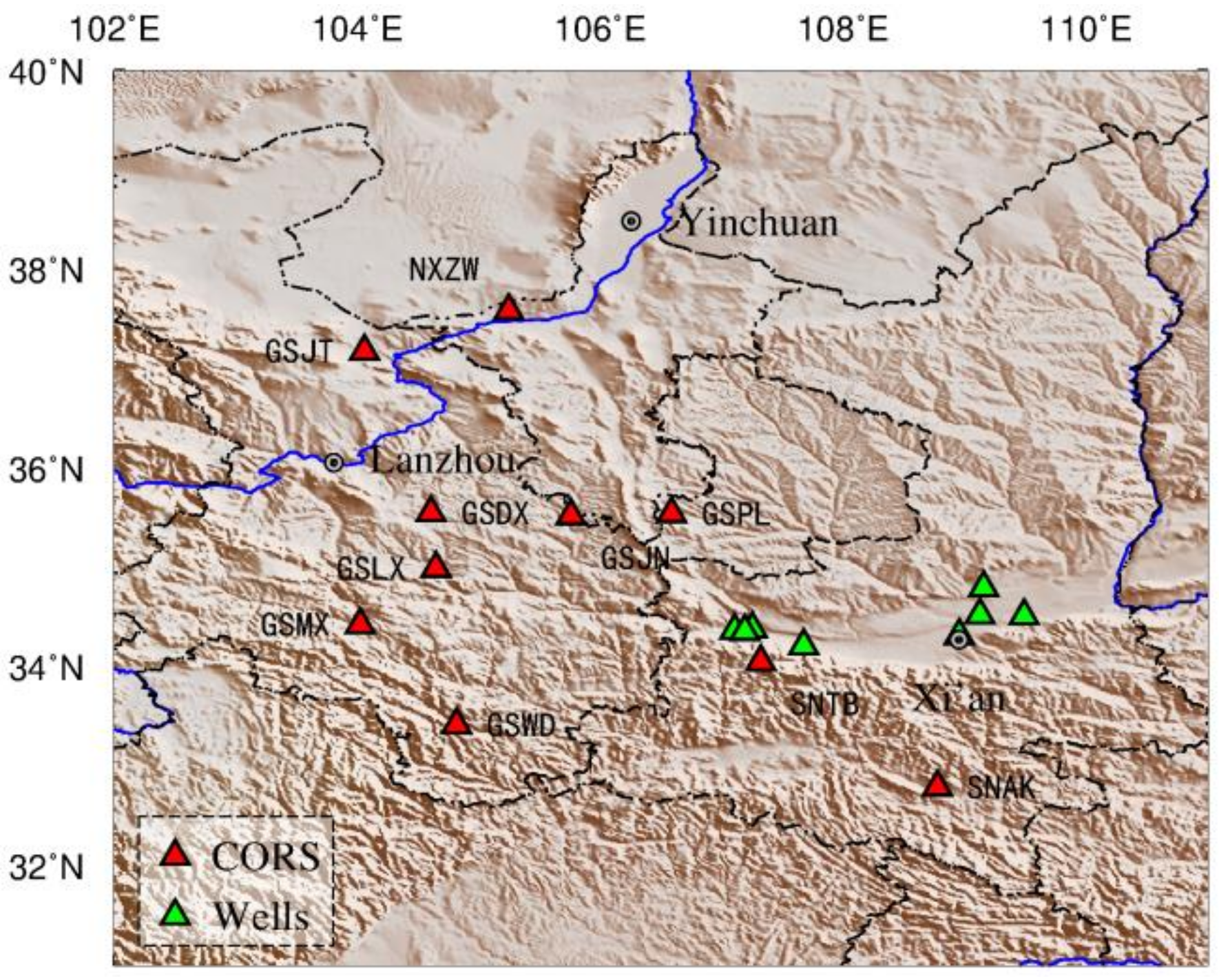
2.1. Data

2.1.1. GNSS Data

We adopted geodetic height data from 10 CORS stations, resulting from continuous GNSS observations in the SGN region from 2011 to 2014. Data processing was carried out via GAMIT/GLOBK software 10.7 version [23]. Single-day region relaxation solutions for station and satellite orbits were obtained using each GNSS station’s daily data. Based on the GAMIT-derived baseline solutions, GLOBK was employed in joint adjustment to obtain time series of station coordinate changes under the ITRF2014 framework [24]. Solid tides, ocean tidal signals and atmospheric tidal signals were removed using the IERS 2010 protocol. Limited by the acquired station data, only 10 CORS data of relatively good quality can be used for experimental research. An SSA method combined with a 3 times standard deviation criterion was adopted to detect and eliminate outliers in the geodetic height time series from GNSS [25]. For shifts in these time series, a fitting method based on a GNSS coordinate time series function model was used to remove the linear trend and step terms and reduce the influence of tectonic movement, earthquakes and instrument replacements [13]. The SSA algorithm [26] was used for interpolation compensation for missing data. The locations of the Continuously Operating Reference Stations (CORS) in the SGN region are shown in red in Figure 1, and the locations of wells for monitoring groundwater level are shown in green. In addition, the main parameters used in the GAMIT calculation are given in

Table 1. The main parameters used in the GAMIT calculation [26,27].

Parameter	Processing Mode
Tropospheric model	Saastamoinen + GPT2w + estimation
Ionosphere delay model	LC_AUTCLN
Ambiguity resolution	LAMBDA method
Satellite cut-off elevation angle (°)	10
Sampling interval data	15 s
Solid tide model	IERS2010
Ocean tide model	FES2004 (otl_FES2004.grid)
Atmospheric mapping function	VMF1
Solar radiation pressure model	ECOMC model
PCO/PCV	IGS14 atx
Framework of prior coordinates	ITRF2014
Inertial framework	J2000

.

2.1.2. GRACE Data and Post-Processing

The GSM solutions from the GRACE mission were used in this paper, as downloaded from the Center for Space Research (CSR, the University of Texas at Austin). A level-2 (RL06) monthly gravity field model GSM was regularized by the SH coefficient, which deducts the effects of solid tides, ocean tides, solid polar tides, non-tidal atmospheres, and oceanic influences, as well as gravity disturbances caused by other entities, such as the sun and the moon.

We used GRACE CSR RL06 data (up to a degree and order of 60) to invert regional TWS, according to Equation (2) [28]. The noise of high-degree and high-order coefficients was filtered by fan filtering with a smooth radius of 300 km [29,30]. The correlation error was removed via P₃M₁₅ decorrelation filtering [31]. The coefficients of the first degree were replaced by the satellite laser ranging (SLR) estimates [32]. In addition, we replaced the C₂₀ coefficients of GSM with GRACE Technique Note 14 [33]. For missing monthly data, the spherical harmonic (SH) coefficients were filled in by averaging the values from the two adjacent months [34,35].

2.1.3. Atmospheric Pressure Data

The monthly global atmospheric pressure model was derived from European Centre for Medium-Range Weather Forecasts (ECMWF)’s reanalyzed ERA-Interim surface pressure product data, with a spatial resolution of 0.25° × 0.25° (https://www.ecmwf.int/ (accessed on 1 February 2022)) [36]. The time period of the data was from January 2011 to December 2014, the same as GNSS data. Using these data, we calculated the crustal vertical displacement from atmospheric loading changes, which included non-tidal atmospheric pressure changes as well as the tidal component [37].

2.1.4. MSLA Data

Merged monthly sea level anomalies (MSLA) grid data provided by AVISO (Archiving Validation and Interpretation of Satellite Oceanography) with 0.25° × 0.25° spatial resolution (https://www.aviso.altimetry.fr/ (accessed on 5 January 2022)) were used in this paper. These data were calculated from observations of multiple satellite altimeters (TOPEX/Poseidon, Jason-1/2 and Envisat) covering the period from January 2011 to December 2014. Necessary geophysical corrections, such as tidal corrections and inverse barometer corrections, were applied by AVISO [38]. In addition, we used MSLA data from the AVISO website to calculate the crustal vertical displacement driven by non-tidal ocean load.

2.1.5. GLDAS Noah Hydrological Model

The monthly global land data assimilation system (GLDAS) hydrological model was constructed by NASA (National Aeronautics and Space Administration) and the National Centers for Environmental Prediction (NCEP), reflecting monthly changes in soil water, ice and snow, and vegetation water content on the Earth’s surface (https://mirador.gsfc.nasa.gov/ (accessed on 6 January 2022)), incorporating four terrestrial surface modes—NOAH, VIC, CLM and MOSAIC. Among several land surface models from GLDAS, the NOAH model is the most commonly used for hydrological applications [39,40]. We used the monthly GLDAS NOAH 2.1 hydrology model with a spatial resolution of 0.25° × 0.25° in this paper [30]. Observations from the GLDAS model are available from January 1979 until present. The TWS estimates from GLDAS NOAH included three main compartments, namely CAN, SM, and SN. In the GLDAS NOAH model, no ice sheet flow and mass balance were included; Antarctica and Greenland were thus excluded from computations. Moreover, GLDAS types of hydrology loading do not include surface water and groundwater compartments. Therefore, the total vertical surface displacement caused by changes in the load from soil water, ice and snow, and vegetation water could be calculated.

2.1.6. WGHM Hydrological Model

We made use of the WaterGAP global hydrology model (WGHM) developed at the University of Frankfurt [41]. The WGHM version adopted in this paper was model WaterGAP v2.2d. Irrigation accounts for 60~70% of global water withdrawal uses [41]. The WaterGAP model contains information on CAN, SN, SM, GW, and SW parameters [29]. The model was implemented to provide information on ground and surface waters and the exchange of water between them. Five different uncertainty sources were identified in WaterGAP: climate forcing, land cover, model structure, human water use, and data calibration concerning observed water discharge. WaterGAP 2.2 had a 0.5° × 0.5° spatial resolution and spanned the time period from January 2011 to December 2014, which was almost the same as the GRACE observation period.

2.1.7. In Situ Data of Groundwater Level

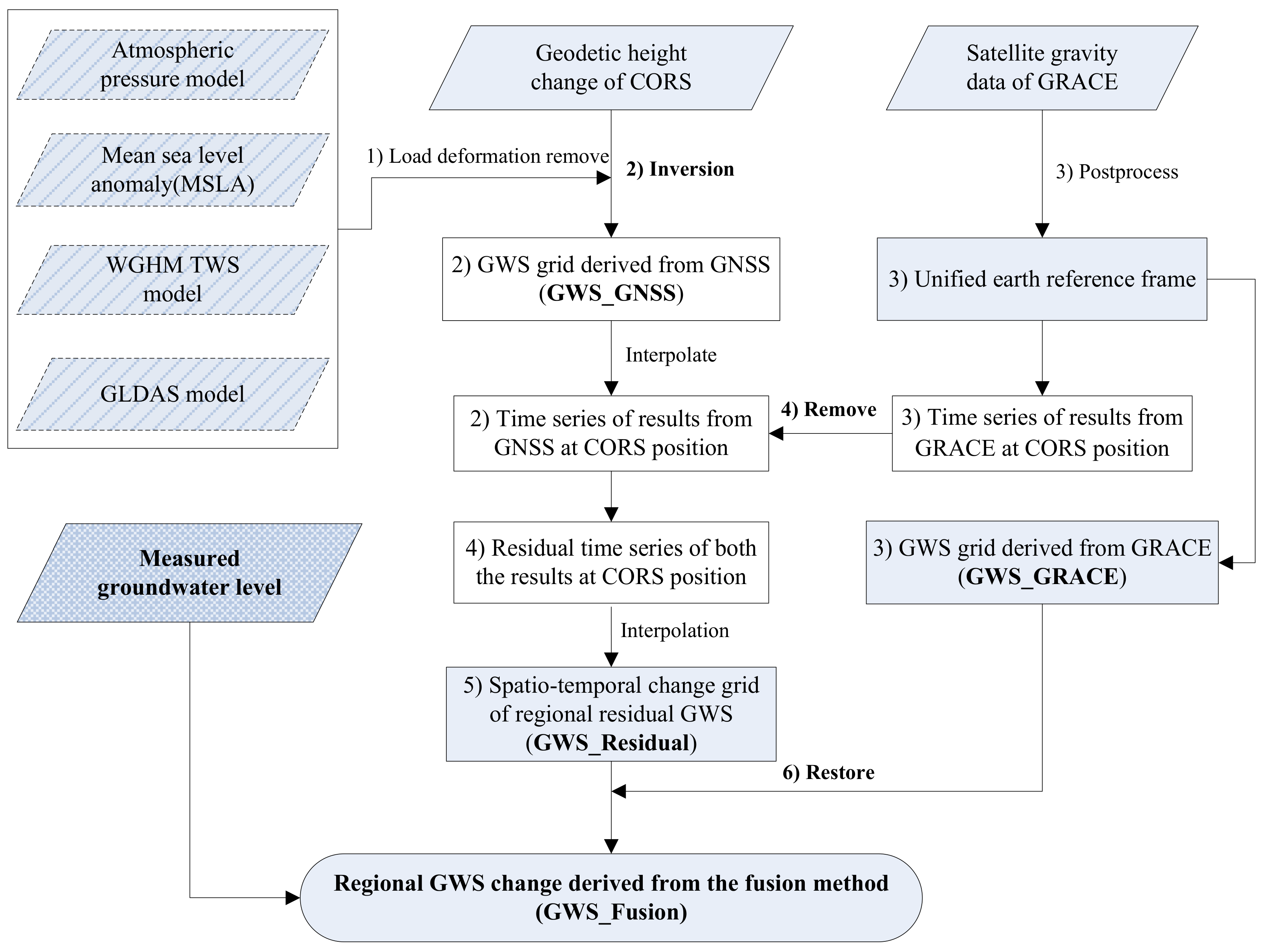
The in situ groundwater level data were obtained from the groundwater level yearbook of Shaanxi Province. The data comprised the groundwater depth observed by eight monitoring wells in the Guanzhong area. The observation time resolution was five days and its unit was meters. To compare the GNSS, GRACE, and fusion inversion results quantitatively, the in situ groundwater level data were averaged and the monthly variation data were obtained.

2.2. Fusion Method

2.2.1. The Inversion from GNSS Data

The goal of this paper was to study the spatiotemporal changes in GWS in the SGN region. Because the number of regional stations was significantly lower than that of the spatial grid points, the constructed normal equation had rank deficiency. Therefore, the Laplace prior matrix and regularization method are introduced in this paper to solve the ill-posed problem of the algorithm equation [42,43]. Based on Green’s load function deformation theory, the inversion model using the residual vertical displacement from GNSS is constructed as

$${\left(\left(A_{u}x-y_u\right)/{\sigma }_u\right)}^2+{\alpha }_{ui}{}^2{\left(L(x)\right)}^2\to \min$$

(1)

where ${\sigma }_u$ is the vector standard deviation of vertical displacement observations; $A_u$ is Green’s radial function coefficient matrix; $x$ is the equivalent water height of parameters to be solved corresponding to grid points in study area; $y_u$ is the residual vertical displacement observation from GNSS; ${\alpha }_u$ is the corresponding regularization parameters; and $L(x)$ is the Laplacian matrix [43].

2.2.2. The Estimation from GRACE Data

Aliasing stripe errors in GRACE data should be filtered to improve the signal-to-noise ratio of the inversion results. Due to the limitations of single filtering, fan and decorrelation filtering are combined in this paper to reduce the influence of high-degree noise in the time-variable gravity field model. The calculation model of the combined filtering method is as follows [44,45]:

$$\Delta h_w(\phi ,\lambda )=\frac{R{\rho }_e}{3{\rho }_w}{\displaystyle {\sum }_{n=0}^N{W}_n{\displaystyle {\sum }_{m=0}^n\frac{2n+1}{1+{k^{\prime }}_n}[\Delta C_{nm}\cos m\lambda +}}\Delta S_{nm}\sin m\lambda ]·W_m·{\overline{P}}_{nm}(\cos \phi )$$

(2)

where $(\phi ,\lambda )$ are the geocentric colatitude and longitude of ground points; $(\Delta C_{nm},\Delta S_{nm})$ are variations in the normalized potential coefficient with degree n and order m; ${\overline{P}}_{nm}(·)$ is the normalized associative Legendre functions; $k_n$ is the load LOVE number with degree n [46]; ${\rho }_w\approx {10}^3\mathrm{kg}/{\mathrm{m}}^3$ is the density of water; ${\rho }_e\approx 5.5\times {10}^3\mathrm{kg}/{\mathrm{m}}^3$ is the average density of solid earth; R is the radius of the Earth; and $W_n$, $W_m$ are filter kernel functions with degree n and order m. In the current calculation of surface mass change derived from GRACE, the kn load Love number used is based on the preliminary reference Earth model (PREM), and its order is as high as 40,000. Only the numerical results of the first 10 orders of the kn load Love number are given in this paper. The results from order 0 to order 10 are 0.0000, −0.3057, −0.1963, −0.1339, −0.1049, −0.9050, −0.8223, −0.7671, −0.7260 and −0.6930 [46].

2.2.3. Fusion Method Based on GNSS and GRACE Data

The specific process by which the fusion of GNSS and GRACE data was achieved to invert regional GWS variation was based on remove–restore theory, which can be summarized as follows: (1) The SSA algorithm is used to decompose and reconstruct the post-processed geodetic height time series from GNSS, and the corresponding time series of multiple principal components are obtained. The weighted correlation analysis method is used to calculate the correlation coefficient between each principal component to determine the degree of separation, effectively extracting the nonlinear deformation signals. The influence of deformation caused by environmental load changes is comprehensively calculated, and the residual displacement observation in the GNSS inversion model is obtained by deducting the load influence. (2) Based on Green’s function method, the residual displacement observation from GNSS is used to invert regional GWS changes at a spatial resolution of 0.5° × 0.5°, and the independent inversion result derived from GNSS is recorded as GWS_GNSS. It should be noted that GNSS inversion involves the rank defect of the normal equation, and the regularization method is used in this paper to solve this problem. (3) GRACE gravity data are post-processed, and the reference frame is unified to further invert the regional GWS changes with the same spatial resolution. This is named GWS_GRACE. (4) By introducing the remove–restore theory, the GWS changes observed by GRACE are removed from the time series of GWS changes derived from GNSS at the CORS stations, and the residual time series from ten CORS stations are obtained. (5) The kriging interpolation method is used to interpolate the residual series from ten stations into a regional grid of residual GWS changes with a spatial resolution of 0.5° × 0.5°, which is recorded as GWS_Residual. (6) The “GWS_Residual” residual grid value is added back to the “GWS_GRACE” grid to obtain the regional GWS change based on the fusion method, which is recorded as “GWS_Fusion”.

Because the study area of this paper was the Shaanxi–Gansu–Ningxia region, the selected latitude and longitude range was 102°~111°E, 31°~40°N. To solve the problem of border areas without stations, we increased the integral radius of Green’s function. Of course, in areas where there are no stations, the reliability of the GNSS inversion results is limited, which is why we added GRACE data for fusion inversion. The specific process is shown in Figure 2.

3. Fusion Results and Analysis

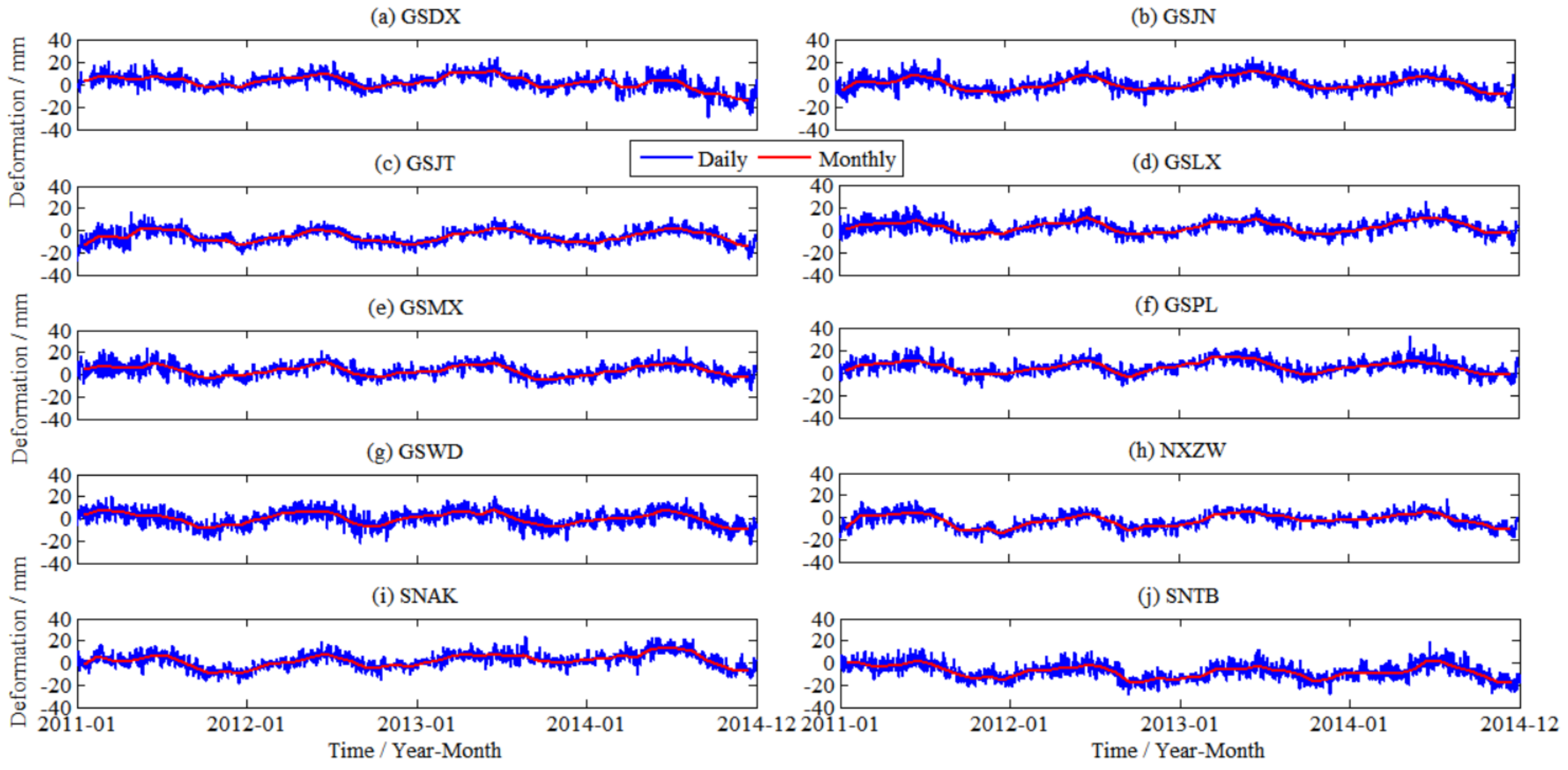
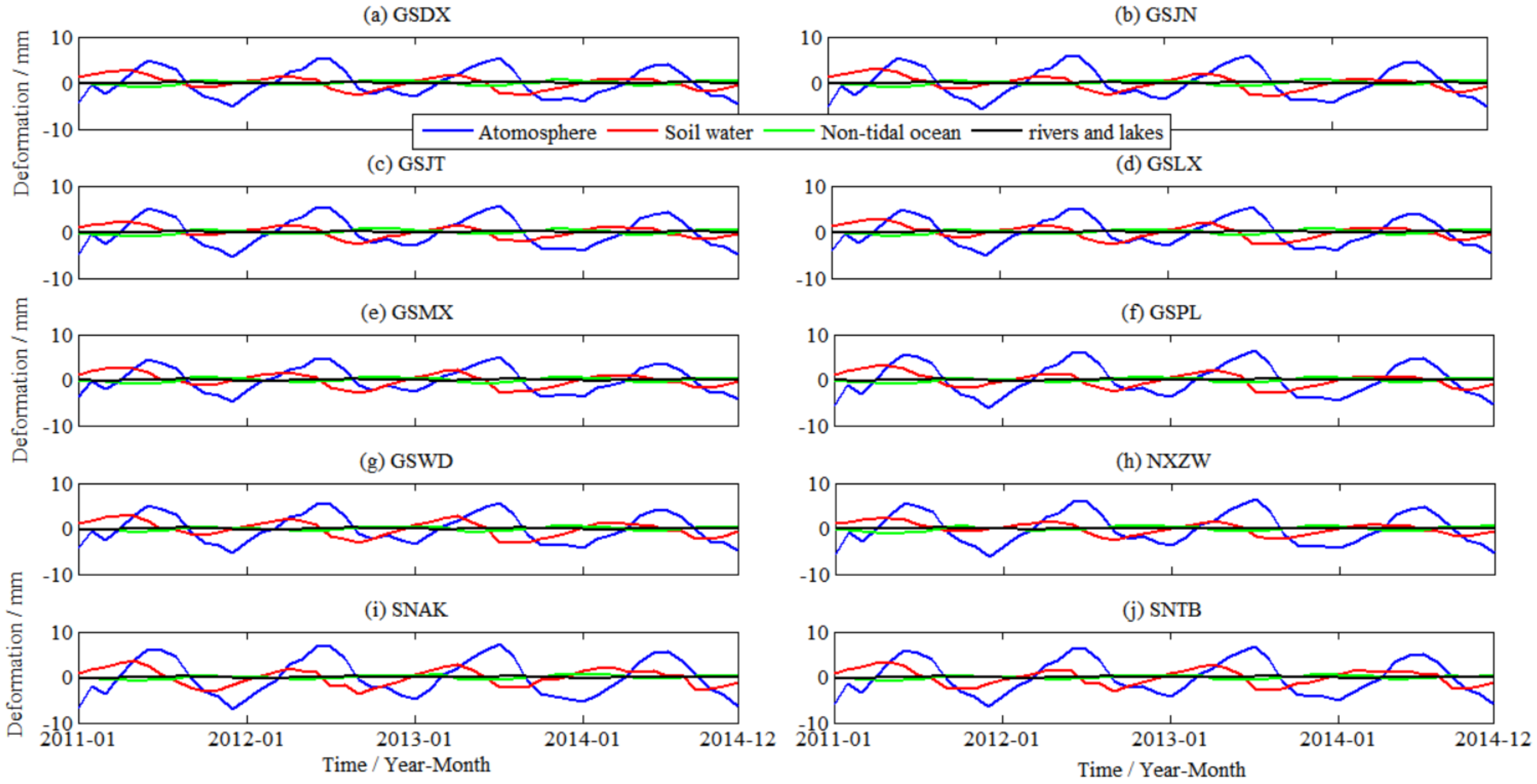
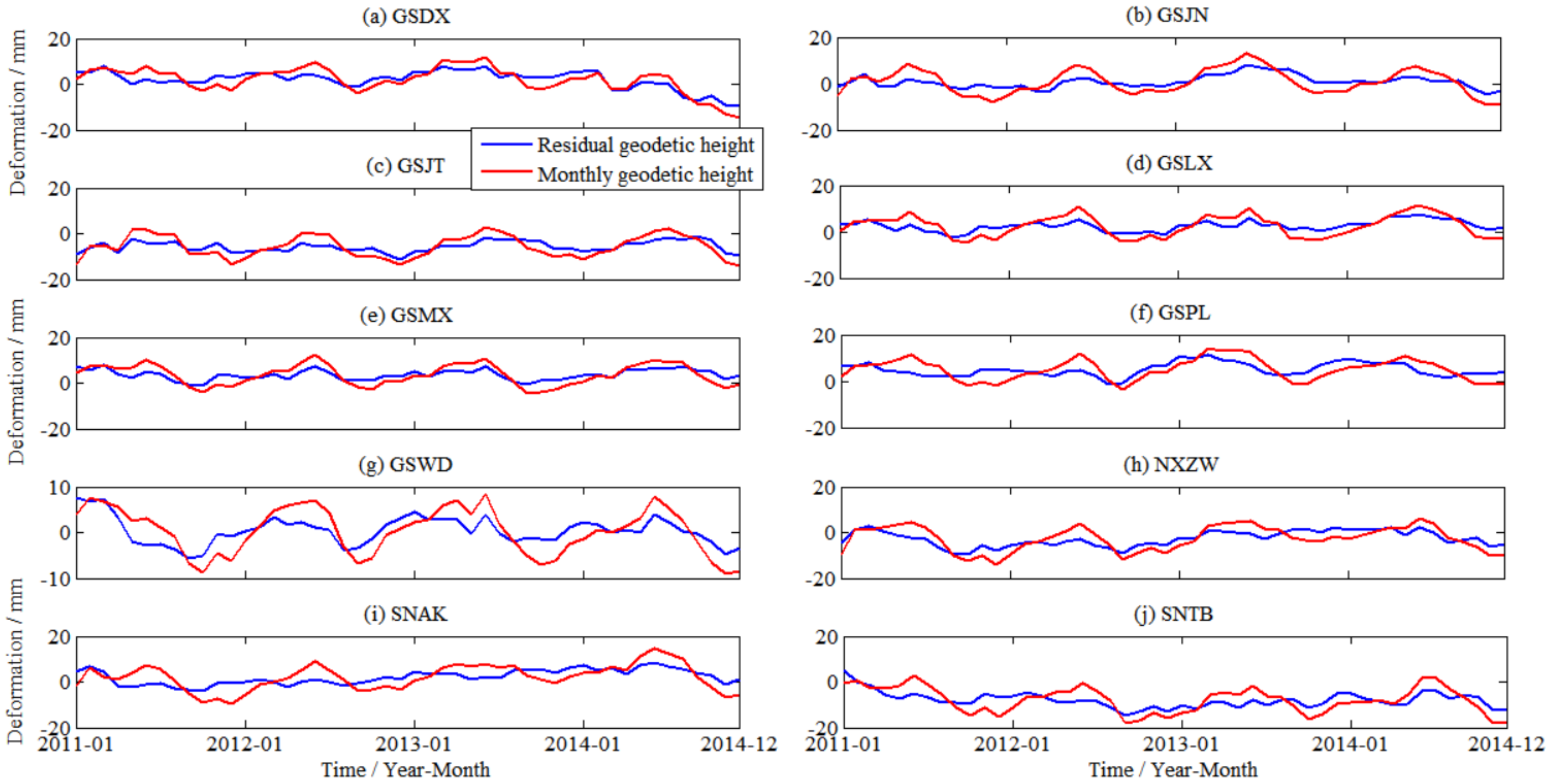
3.1. GNSS Data Extraction and Environmental Loading Deformation Calculation

In order to improve the accuracy of GWS changes derived from GNSS, the SSA method was used to carry out gross error detection, step term correction, filtering, and noise reduction on the original geodetic height time series of the ten CORS stations. In addition, monthly averaging is adopted, and the monthly variation in geodetic height is obtained, as shown by the red curve in Figure 3. The blue curve represents the time series after gross error detection and step term correction without filtering and monthly average processing.

In this paper, the vertical deformations from CORS stations caused by different environmental loads were comprehensively calculated, such as loads from atmospheric pressure, non-tidal ocean, soil water, ice and snow, vegetation, and water from rivers, lakes, and reservoirs. Deducting the same time benchmarks of all monthly averages, the monthly deformation sequence was obtained. These load deformation effects are shown in Figure 4.

To obtain the residual deformation observations in the GNSS inversion model, it was necessary to deduct the total load influence shown in Figure 4 from the processed time series from GNSS. The time series of residual geodetic height was obtained as shown in Figure 5.

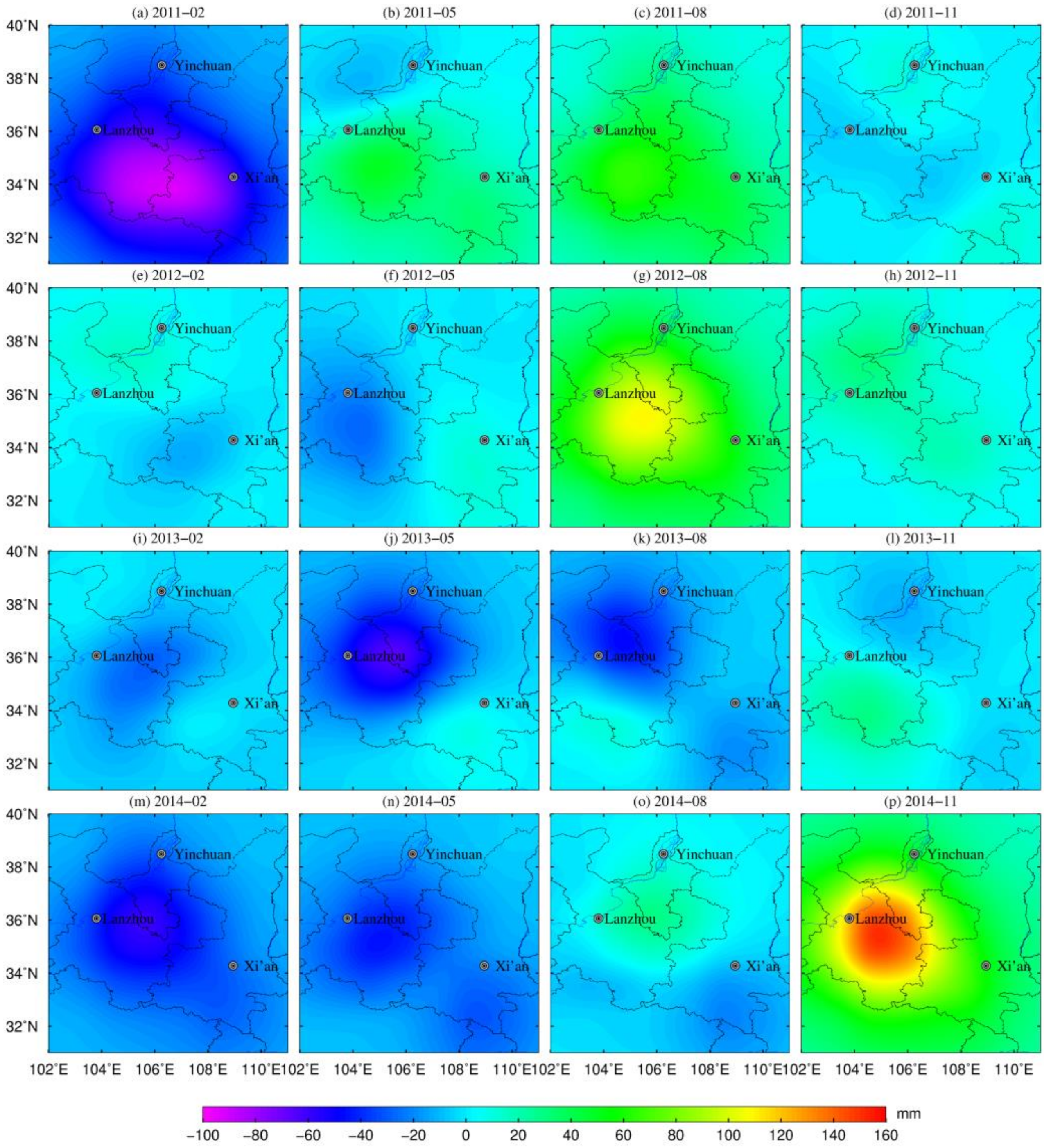
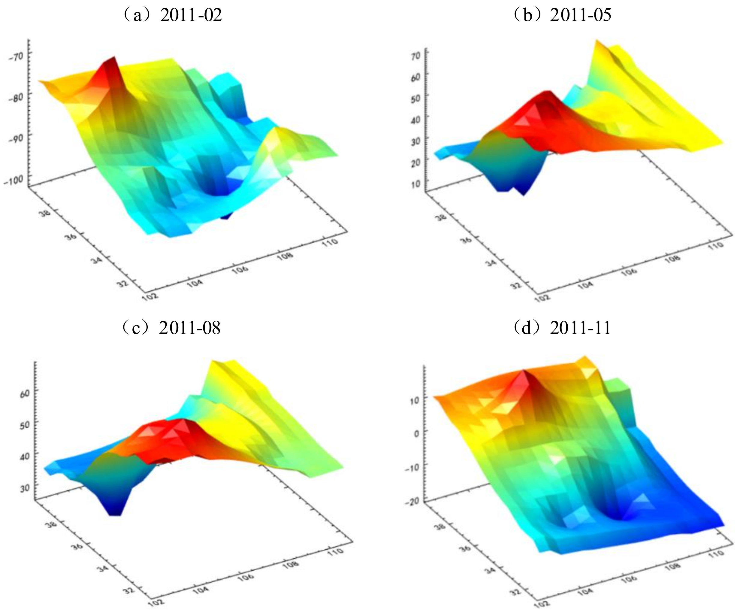
3.2. Regional GWS Variation Derived from GNSS

Based on the residual time series of geodetic height from GNSS, the Green’s function integral method was adopted to construct the GNSS inversion model, and the regularization method was adopted to solve the regional GWS variations with the resolution of 0.5° × 0.5°. The integral radius was set to 1 degree. The spatial grid of regional GWS changes inverted by GNSS is shown in Figure 6. To intuitively show the seasonal characteristics of the inversion results, the spatial distribution of the inversion results from February, May, August, and November from 2011 to 2014 are given in this paper. The x-axis represents the longitude range (102°~111°E), the y-axis represents the latitude range (31°~40°N), and the z-axis represents the actual numerical results of GWS variations.

It can be seen that the results derived from GNSS better reflect the spatiotemporal distribution characteristics of the regional GWS from 2011 to 2014. However, signals with large amplitudes were generally distributed close to the stations, and the local effects were obvious. In areas where stations were missing or sparsely distributed, such as the southwest and northeast of study area, the signal strength was relatively weak. In addition, there may have been greater uncertainty, and the reliability of the inversion results was therefore constrained.

On this basis, the spatial grid of regional GWS independently derived from GNSS was interpolated to the CORS stations via the Kriging interpolation method, and the time series of GWS changes at the ten CORS stations were obtained, as shown in Figure 7. At this time, the linear terms of the results were derived from GNSS. It can be observed from Figure 7 that the time series of GWS changes in each station derived from GNSS fluctuated obviously, and while there were amplitude changes of different degrees, the overall trend was consistent.

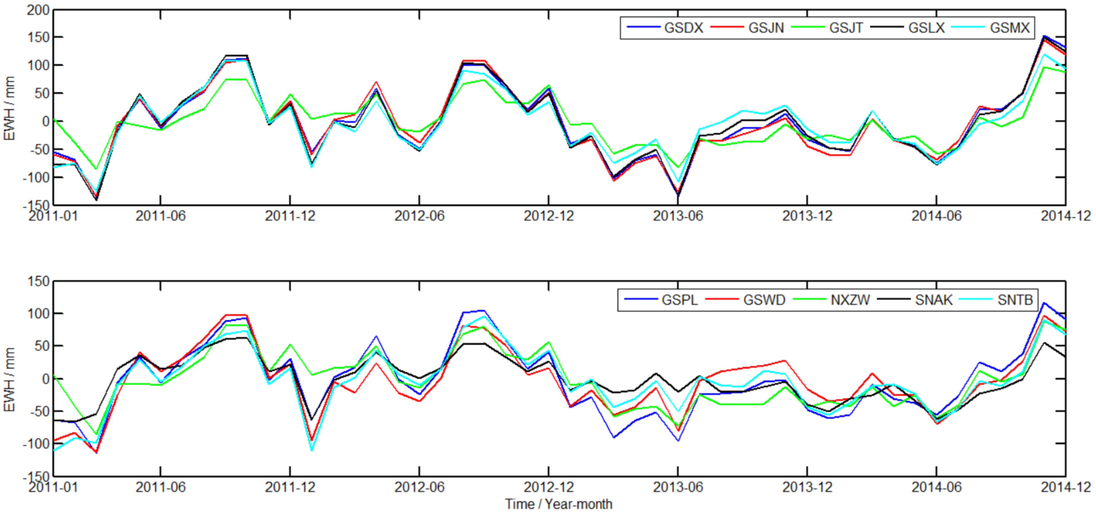
3.3. Regional GWS Changes Derived from GRACE

In this paper, the monthly gravity field model of GRACE from January 2011 to December 2014 was used to invert regional TWS changes with the same resolution. The relative variation in the monthly gravity field could be acquired after deducting the multi-year average [45]. The glacial isostatic adjustment (GIA) effect was subtracted depending on the crustal equilibrium model from Paulson [47]. Furthermore, a single-scale factor k = 1.21 [48] was used to redu ce leakage errors caused by filtering.

To obtain the change in GWS in the study area, it was necessary to deduct the soil water, ice and snow, vegetation water content, and the water storage of rivers, lakes, and reservoirs from TWS changes derived from GRACE. The surface water storage changes with a resolution of 0.5° × 0.5° (including soil water, ice and snow, and vegetation) in the study area were obtained by the GLDAS model. The water storage changes in rivers, lakes, and reservoir were extracted from the WGHM model. In this paper, taking July in 2011 as an example, the spatial distributions of the water storage of soil water, snow, rivers, lakes, and reservoirs are shown in Figure 8.

The spatial distribution of the TWS changes derived from GRACE after recovering the leakage signal are shown in Figure 9. Taking 2011 as an example, the spatial changes in TWS from GRACE in February, May, August, and November are given in the figure.

As can be seen from Figure 9, taking 2011 as an example, the change in TWS from GRACE has obvious spatiotemporal heterogeneity. In May 2011 and November 2011, the signal intensity in the SGN region showed a decreasing trend from east to west, and the change in water storage near Xi’an showed an obvious loss in May and a surplus in November. In February and August of the same year, there was no abnormal change in water storage, and the spatial distribution was more consistent.

To be consistent with the process for GRACE data, SH expansion, combined filtering, and scale factor correction were performed on the GLDAS model in this paper to further invert changes in soil water and snow and vegetation water content, which were deducted from the GRACE-corrected results. The obtained spatiotemporal distribution of the GWS in the SGN area is shown in Figure 10.

It can be observed from Figure 10 that the GWS changes derived from GRACE showed obvious spatial inhomogeneity within individual months. In winter and autumn, the GWS in most areas increased to varying degrees. In 2011 and February 2014, the GWS in Yinchuan and Xi’an increased most significantly. From 2011 to 2013, the loss of GWS in spring was serious. This strong loss signal appeared in the Xi’an area in May 2012 and August 2013. In May 2012 and August 2013, the GWS derived from GRACE in Xi’an showed a serious loss, and this loss signal may have been related to the impact of leakage in the signal from adjacent areas caused by GRACE filtering [49].

In addition, we estimated TWS changes by GPS station location using GRACE data in spherical harmonic form to further obtain the single-point time series of GRACE estimation results, rather than interpolate the GRACE results grid into the CORS station positions, as shown in Figure 11.

From Figure 10 and Figure 11, we can see that the spatial characteristics of regional GWS changes derived from GRACE were not refined, and the local characteristics were difficult to highlight. The fluctuation in the temporal distribution was more obvious. The overall time series trend of GWS from GRACE was consistent among stations, but the amplitude was slightly different.

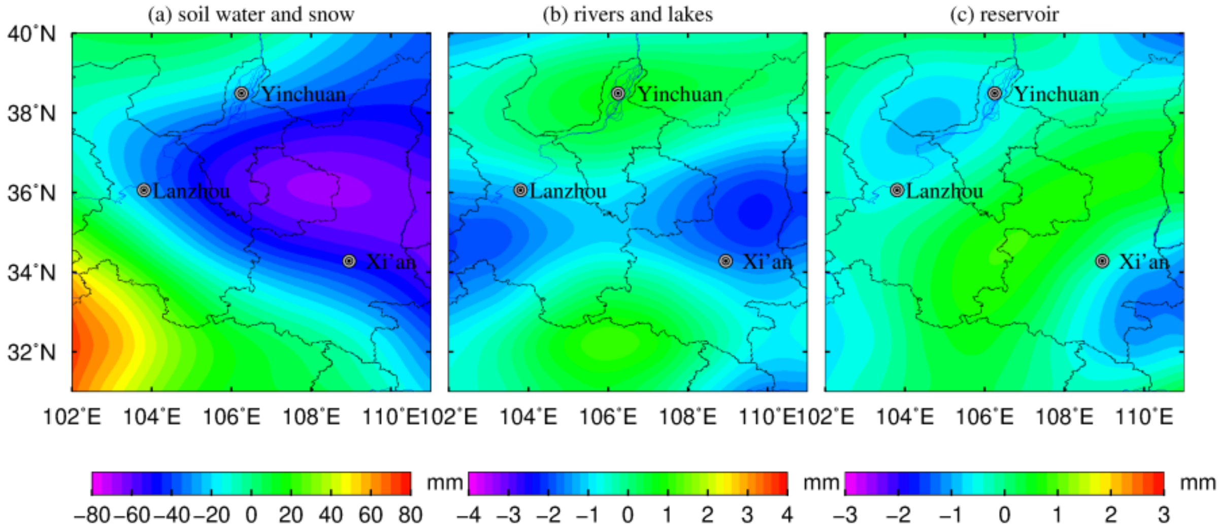
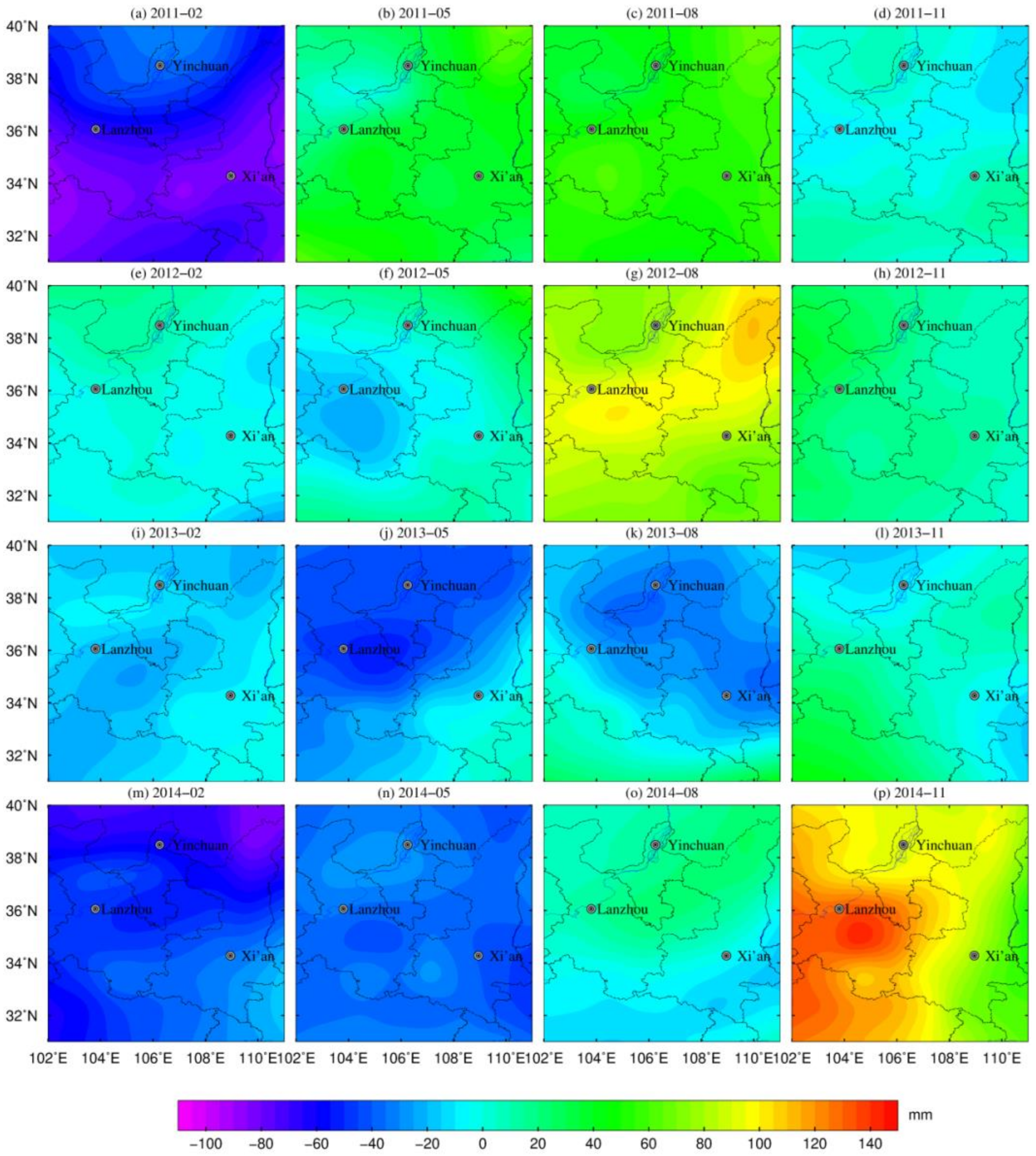
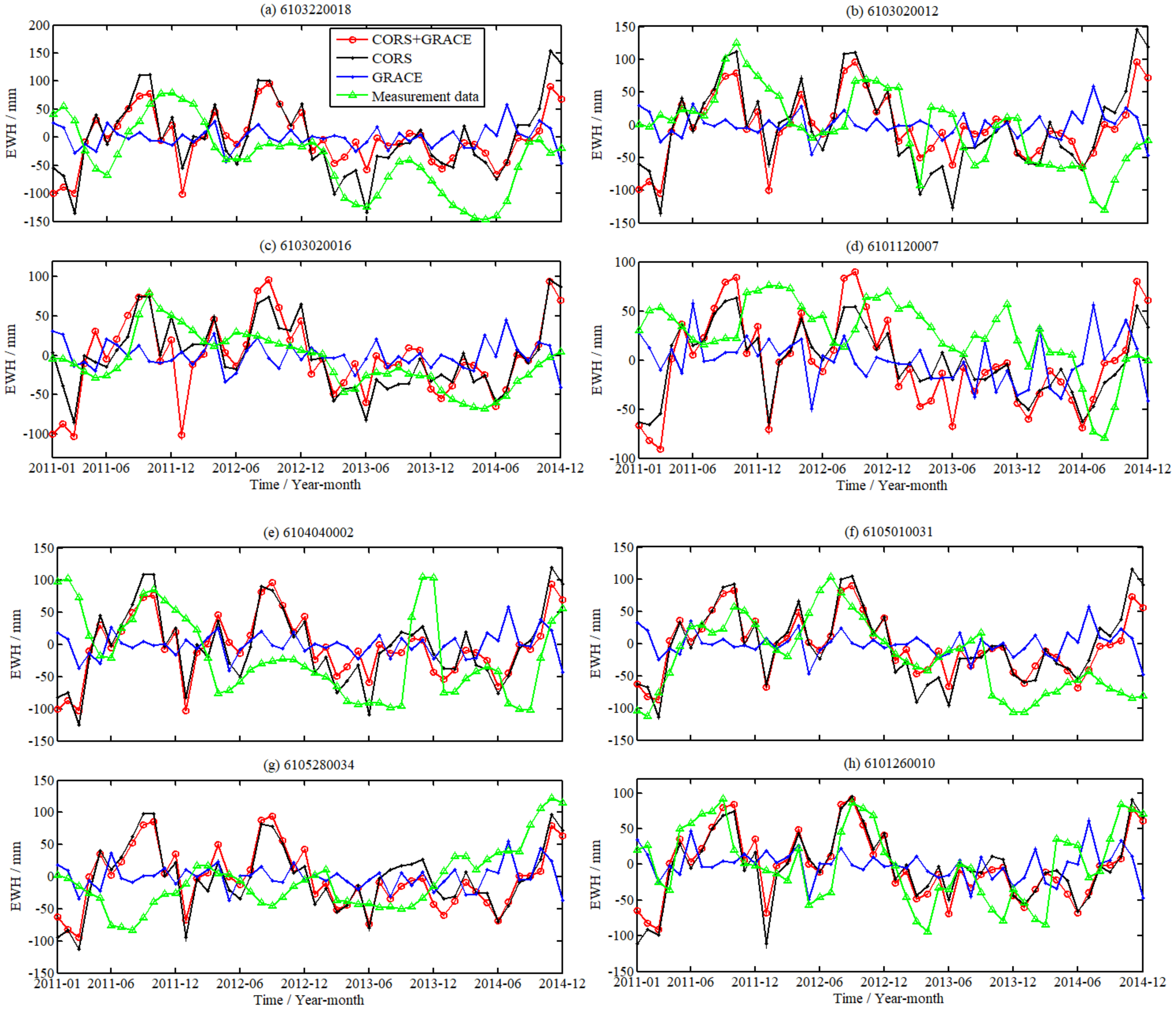
3.4. Regional GWS Changes Based on the Fusion Method

GNSS inversion mainly reflects the local signal characteristics and their short-wave signals, whereas GRACE results are mainly reflected in the mid-long wave signal. In this paper, based on the “remove and restore” method of local gravity field approximation, the residual signal after removing the long-wave signal was obtained by deducting the GRACE single-point results from the single-point time series of GNSS inversion at the position of CORS stations. The regional residual signal grid was then obtained by interpolation. On this basis, re-adding the mid-long wave signal of the GRACE result grid through the “remove-restore” step, the final full-wave band results of the groundwater storage change grid were obtained.

According to the fusion concept presented earlier in Figure 2, this paper needed to fuse the time series of regional GWS changes derived from GNSS and GRACE at the location of the CORS stations. Deducting the GRACE result in Figure 11 from the GNSS inversion result in Figure 7, the residual time series between them at the station location was obtained, as shown in Figure 12.

On this basis, Kriging interpolation was performed on the residual time series at the positions of ten CORS stations to obtain the residual grid value in the region. Taking February, May, August, and November in 2011 year as examples, the spatial distribution maps of the residual GWS variation grid after Kriging interpolation are given in Figure 13.

Figure 13 mainly reflects the residual signals after deducting the long-wave signals in GRACE from the short-wave signals retrieved by GNSS. Taking 2011 as an example, the residual signal had obvious spatial inhomogeneity, and the local signal characteristics were obvious, especially in the northwest and southwest regions of the study area.

Based on the above results, the spatiotemporal grid maps of regional GWS changes derived from GRACE in Figure 10 are added to the residual value grid map in Figure 13. The obtained spatiotemporal distribution of the fusion inversion results are shown in Figure 14.

It can be seen from Figure 14 that the spatial resolution of the regional GWS changes derived from the fusion method based on GNSS and GRACE data is improved compared with that from GRACE in Figure 10, and the detailed features are more prominent. For example, the GWS in southern Lanzhou showed a slight loss in May 2012; meanwhile, the GWS rebounded slightly in southeastern Lanzhou and eastern Yinchuan in August 2012. From February to August 2013, the GWS in the Lanzhou area was in a state of continuous loss, with the largest decrease occurring in May 2013. In February 2013, a slight decrease in the GWS in northeastern Yinchuan occurred, and the magnitude of loss in GWS in southwestern Yinchuan increased slightly in August 2013. In February 2014, the loss signal of GWS was particularly significant in the northeastern part of study area. In May 2014, the loss signal of GWS in southern Lanzhou and Xi’an was still strong. In August 2014, the loss in GWS in southern Xi’an was alleviated, and there was an obvious surplus in the regional water storage in November of the same year. However, the largest increase signal in regional GWS was particularly significant in southeastern Lanzhou in November 2014.

It can be seen that compared with the results derived from GRACE, the fusion inversion results also better captured the detailed characteristics of regional GWS changes, despite sparse and missing areas for CORS stations, such as the southwest and northeast in the study area.

To verify the reliability of the fusion method based on GNSS and GRACE data, the three kinds of spatial grid results derived from the GNSS, GRACE, and fusion methods were interpolated to the location of eight groundwater level monitoring wells in the study area, and the in situ groundwater level data were adopted for verification and analysis. The corresponding results derived from GNSS and GRACE are shown in Figure 15. It should be noted that gross error elimination and monthly average processing were carried out for the in situ groundwater level data.

We collected the measured groundwater level data for gross error detection and elimination and monthly average processing. At the same time, the change water level data were multiplied by the coefficient of “−1” and then compared with the GNSS/GRACE results. It should be noted that because the local soil porosity data were not collected, the measured groundwater level data were not multiplied by soil porosity. Therefore, this paper focuses on the comparison of phase correlation and the comprehensive analysis of the overall trend.

It can be seen from Figure 15 that both the results derived from the fusion method and GNSS were consistent with the overall trend of the in situ groundwater level. In the second halves of 2011 and 2014, when the groundwater level increased significantly, both the results from GNSS and the fusion method all showed a significant increase in GWS. From June 2012 to June 2013, the groundwater level of most monitoring wells decreased significantly, and the GWS derived from GNSS and fusion method also showed obvious losses.

To quantitatively analyze the effect of the fusion method, the correlation coefficient between the results derived from GNSS, GRACE, the fusion method, and the in situ groundwater level data were calculated in this paper, as shown in

Table 2. Correlation coefficients between results from GNSS/GRACE, fusion method and in situ groundwater level data.

IDS of Water Level Monitoring Station	Correlation Coefficients (GNSS/GRACE/Fusion)	IDS of Water Level Monitoring Station	Correlation Coefficients (GNSS/GRACE/Fusion)
6103220018	0.35/−0.02/0.20	6103020012	0.30/−0.18/0.32
6103020016	0.60/−0.06/0.40	6101120007	0.17/−0.06/0.07
6104040002	0.21/−0.11/0.05	6105010031	0.41/−0.02/0.53
6105280034	−0.06/0.15/−0.04	6101260010	0.49/0.21/0.56

. It can be seen from the GWS change trend in Figure 15 and the correlation coefficients in Table 2 that the results derived from GNSS were closer to the in situ groundwater level changes than those derived from GRACE. However, due to the small number and uneven distribution of CORS stations in the study area, the local effect on the inversion results from GNSS was significant. The GRACE data were thus added to improve the imbalance in the spatial signals of the GNSS results. From the perspective of individual stations, especially groundwater level monitoring stations 6105010031 and 6101260010, which were located in areas where CORS stations were missing, the accuracy of the fusion results was higher than that of the single inversion method. The accuracy of the fusion results from the four stations 6103220018, 6103020016, 6101120007, and 6104040002 was not as good as that of the GNSS inversion results. It may be that these four hydrological stations were located near the CORS station, which was mainly reflected in the GNSS inversion signals. The fusion method proposed in this paper is more suitable for areas where CORS stations are missing or sparsely distributed. In addition, the comparison results of only four hydrological stations cannot effectively show that GNSS inversion is more accurate than fusion results. It is necessary to further strengthen the comparative study in the missing area for CORS stations in future research.

4. Discussions on the Fusion Method

This paper focuses on testing and validating the reliability of the proposed fusion method for monitoring regional GWS changes based on GNSS and GRACE data. Furthermore, the corresponding implementation process is given. It can be seen from the verification and analysis for in situ groundwater level that the results from the fusion method can overcome the local effect caused by inversion from GNSS well. Moreover, the uncertainty of the corresponding regional inversion results caused by sparsely distributed or missing stations may be reduced. Compared with the results from GRACE, the spatial details are more prominent in the fusion results.

In our paper, we found that there was a large difference between results from regions such as Xi’an and Lanzhou derived by the fusion method and GRACE. Li [23] also found that obvious differences in spatial distributions still existed in some major cities from the SGN region when comparing total surface mass changes derived from GPS to GRACE/GFO SH solutions and mascon solutions.

Therefore, in future research, several factors need to be considered and improved, including phase difference correction, weight setting, and finer processing for in situ groundwater level data. In fact, there was a time delay between the results from both GNSS and GRACE, and phase difference correction should thus be performed. In view of the different sensitivities of GNSS and GRACE to regional GWS changes, the weight ratio for GNSS and GRACE data should be considered in the actual fusion inversion. The optimal weight ratio can be determined by the variance component estimation method. Strictly speaking, the in situ groundwater level data obtained from monitoring wells is derived from water level changes contained in the soil pores of underground aquifers. If equivalent water height data for GWS changes derived from the inversion method are being quantitatively compared with in situ groundwater level from wells data, the in situ groundwater level data should be multiplied by the corresponding soil porosity.

In addition, as the data collected in this paper were limited by the distribution density of CORS stations and the length of the time series, the accuracy of the inversion results may have been affected. Meanwhile, when comparing results of the fusion method with those from GNSS, more in situ groundwater level data should be added for areas where CORS stations are missing or scarce to help to enhance the contrast and credibility. Furthermore, because the spatial resolutions of the GNSS and GRACE monitoring methods were obviously different, taking the Amazon Basin as an example, Zhang and Sun [50] found that the load displacements obtained by GRACE and GNSS were significantly different in both spatial averages and single points. The fusion method proposed in this paper involves the process of inverting GWS data using the two techniques on a single point, which also increases the uncertainty of the results obtained by the fusion method. These factors will ultimately affect the accuracy of the fusion inversion results, which will be further studied in future research.

5. Conclusions

Considering that the reliability of applying Green’s function method to GNSS data to invert regional GWS changes is limited by the number and distribution of CORS stations, a new method for inverting regional GWS changes by fusing GNSS and GRACE data was proposed in this paper. Here, we took the SGN region as an example, and ten CORS stations and eight groundwater level monitoring wells were used for testing and analysis. Compared with the results from GRACE, the spatial signal from the fusion method was more detailed. Compared with that in GNSS, the local signal effect was weakened. In addition, the spatial distribution of the results derived from the fusion method was more uniform, especially in the southwest and northeast area, where CORS stations were missing or sparsely distributed. In addition, the results from the fusion method and GNSS were more consistent with the change trend of the in situ groundwater level. More specifically, in the wells “6105010031” and “6101260010” located in the area where CORS stations were missing, the accuracy of the fusion results from the two stations was higher than the accuracy of GNSS or GRACE. Therefore, it is reasonable to conclude that the fusion method can compensate for the shortcomings of independent inversion from GRACE. In addition, the fusion method may be more effective for areas where CORS stations are missing or sparsely distributed. In the follow-up work, it is necessary to deeply analyze the factors affecting the accuracy of fusion inversion and effectively correct them.

References

1. Zhong, M.; Duan, J.; Xu, H.; Peng, P.; Yan, H.; Zhu, Y. Trend of China land water storage redistribution at medi- and large-spatial scales in recent five years by satellite gravity observations. Chin. Sci. Bull. 2009, 54, 816–821. [Google Scholar] [CrossRef] [Green Version]
2. Yin, W.; Han, S.C.; Zheng, W.; Yeo, I.Y.; Hu, L.; Tangdamrongsub, N.; Ghobadi-Far, K. Improved water storage estimates within the North China Plain by assimilating GRACE data into the CABLE model. J. Hydrol. 2020, 590, 125348. [Google Scholar] [CrossRef]
3. Feng, W.; Wang, C.Q.; Mu, D.P.; Zhong, M.; Zhong, Y.L.; Xu, H.Z. Groundwater storage variations in the North China plain from GRACE with spatial constraints. Chin. J. Geophys. 2017, 60, 1630–1642. [Google Scholar]
4. Xu, C.; Gong, Z. Review of the Post-processing methods on GRACE time varied gravity data. Geomat. Inf. Sci. Wuhan Univ. 2016, 41, 503–510. [Google Scholar]
5. Cheng, P.; Wen, H.; Liu, H.; Dong, J. Research situation and future development of satellite geodesy. Geomat. Inf. Sci. Wuhan Univ. 2019, 44, 48–54. [Google Scholar]
6. Kornfeld, R.P.; Arnold, B.W.; Gross, M.A.; Dahya, N.T.; Klipstein, W.M.; Gath, P.F.; Bettadpur, S. GRACE-FO: The Gravity Recovery and Climate Experiment Follow-On mission. J. Spacecr. Rocket. 2019, 56, 931–951. [Google Scholar] [CrossRef]
7. Li, F.; Kusche, J.; Rietbroek, R.; Wang, Z.; Forootan, E.; Schulze, K.; Lück, C. Comparison of data-driven techniques to reconstruct (1992–2002) and predict (2017–2018) GRACE-like gridded total water storage changes using climate inputs. Water Resour. Res. 2020, 56, e2019WR026551. [Google Scholar] [CrossRef] [Green Version]
8. Jiang, Z.; Hsu, Y.J.; Yuan, L.; Huang, D. Monitoring time-varying terrestrial water storage changes using daily GNSS measurements in Yunnan, southwest China. Remote Sens. Environ. 2021, 254, 112249. [Google Scholar] [CrossRef]
9. Adusumilli, S.; Borsa, A.A.; Fish, M.A.; McMillan, H.K.; Silverii1et, F. A decade of water storage changes across the contiguous United States from GPS and satellite gravity. Geophys. Res. Lett. 2019, 46, 13006–13015. [Google Scholar] [CrossRef]
10. Famiglietti, J.S.; Lo, M.; Ho, S.L.; Bethune, J.; Anderson, K.J.; Syed, T.H.; Rodell, M. Satellites measure recent rates of groundwater depletion in California’s Central Valley. Geophys. Res. Lett. 2011, 38, L03403–L03406. [Google Scholar]
11. Tiwari, V.M.; Wahr, J.; Swenson, S. Dwindling groundwater resources in northern India, from satellite gravity observations. Geophys. Res. Lett. 2009, 36, 184–201. [Google Scholar] [CrossRef] [Green Version]
12. Hsieh, W. Nonlinear multichannel and time series analysis by neural network methods. Rev. Geophys. 2004, 42, 1003–1027. [Google Scholar] [CrossRef] [Green Version]
13. Jiang, W.; Wang, K.; Li, Z.; Zhou, X.; Ma, Y.; Ma, J. Prospect and Theory of GNSS Coordinate Time Series Analysis. Geomat. Inf. Sci. Wuhan Univ. 2018, 43, 2112–2123. [Google Scholar]
14. Liu, R.; Zou, R.; Li, J.; Zhang, C.; Zhao, B.; Zhang, Y. Vertical displacements driven by groundwater storage changes in the North China Plain detected by GPS observations. Remote Sens. 2018, 10, 259. [Google Scholar] [CrossRef] [Green Version]
15. Fu, Y.; Argus, D.F.; Freymueller, J.T.; Heflin, M.B. Horizontal motion in elastic response to seasonal loading of rain water in the Amazon Basin and monsoon water in Southeast Asia observed by GPS and inferred from GRACE. Geophys. Res. Lett. 2013, 40, 6048–6053. [Google Scholar] [CrossRef]
16. Wang, L.; Chen, C.; Zou, R.; Du, J. Surface gravity and deformation effects of water storage changes in China’s Three Gorges Reservoir constrained by modeled results and in situ measurements. J. Appl. Geophys. 2014, 108, 25–34. [Google Scholar] [CrossRef]
17. Jin, S.; Zhang, T. Terrestrial water storage anomalies associated with drought in southwestern USA from GPS observations. Surv. Geophys. 2016, 37, 1139–1156. [Google Scholar] [CrossRef]
18. Chanard, K.; Fleitout, L.; Calais, E.; Rebischung, P.; Avouac, J.P. Toward a global horizontal and vertical elastic loading deformation model derived from GRACE and GNSS station position time series. J. Geophys. Res. Solid Earth 2018, 123, 3225–3237. [Google Scholar] [CrossRef] [Green Version]
19. Rajner, M.; Liwosz, T. Analysis of seasonal position variation for selected GNSS sites in Poland using loading modelling and GRACE data. Geod. Geodyn. 2017, 8, 253–259. [Google Scholar] [CrossRef]
20. Sarkar, T.; Kannaujiya, S.; Taloor, A.K.; Ray, P.K.C.; Chauhan, P. Integrated study of GRACE data derived interannual groundwater storage variability over water stressed Indian regions. Groundw. Sustain. Dev. 2020, 10, 100376–100395. [Google Scholar] [CrossRef]
21. Liu, R.; Zhong, B.; Li, X.; Zheng, K.; Liang, H.; Cao, J.; Lyu, H. Analysis of groundwater changes (2003–2020) in the North China Plain using geodetic measurements. J. Hydrol. Reg. Stud. 2022, 41, 101085. [Google Scholar] [CrossRef]
22. Wang, H.; Xiang, L.; Steffen, H.; Wu, P.; Jiang, L.; Shen, Q.; Hayashi, M. GRACE-based estimates of groundwater variations over North America from 2002 to 2017. Geod. Geodyn. 2022, 13, 11–23. [Google Scholar] [CrossRef]
23. Li, X.; Zhong, B.; Li, J.; Liu, R. Analysis of terrestrial water storage changes in the Shaan-Gan-Ning Region using GPS and GRACE/GFO. Geod. Geodyn. 2022, 11, 179–188. [Google Scholar] [CrossRef]
24. Herring, T.A.; King, R.W.; Floyd, M.A.; McClusky, S.C. Introduction to GAMIT/GLOBK. Available online: http://geoweb.mit.edu/gg/Intro_GG.pdf (accessed on 2 June 2018).
25. Wang, L.; Chen, C.; Thomas, M.; Kaban, M.K.; Güntner, A.; Du, J. Increased water storage of Lake Qinghai during 2004–2012 from GRACE data, hydrological models, radar altimetry and in situ measurements. Geophys. J. Int. 2018, 212, 679–693. [Google Scholar] [CrossRef]
26. Li, W.; Wang, W.; Zhang, C.; Wen, H.; Zhong, Y.; Zhu, Y.; Li, Z. Bridging terrestrial water storage anomaly during GRACE/GRACE-FO gap using SSA method: A case study in China. Sensors 2019, 19, 4144. [Google Scholar] [CrossRef]
27. Li, W.; Dong, J.; Wang, W.; Wen, H.; Liu, H.; Guo, Q.; Zhang, C. Regional Crustal Vertical Deformation Driven by Terrestrial Water Load Depending on CORS Network and Environmental Loading Data: A Case Study of Southeast Zhejiang. Sensors 2021, 21, 7699. [Google Scholar] [CrossRef]
28. Shi, T.; Guo, J.; Yan, H.; Chang, X.; Ji, B.; Liu, X. Assessing Height Variations in Qinghai-Tibet Plateau from Time-Varying Gravity Data and Hydrological Model. Remote Sens. 2022, 14, 4707. [Google Scholar] [CrossRef]
29. Lenczuk, A.; Leszczuk, G.; Klos, A.; Kosek, W.; Bogusz, J. Study on the inter-annual hydrology-induced displacements in Europe using GRACE and hydrological models. J. Appl. Geod. 2020, 14, 393–403. [Google Scholar] [CrossRef]
30. Li, J.; Chen, J.L.; Wilson, C.R. Topographic effects on coseismic gravity change for the 2011 Tohoku-Oki earthquake and comparison with GRACE. J. Geophys. Res. Solid Earth 2016, 121, 5509–5537. [Google Scholar] [CrossRef]
31. Matsuo, K.; Heki, K. Coseismic and postseismic gravity changes of the 2011 Tohoku-Oki Earthquake from satellite gravimetry. AGU Fall Meet. Abstr. 2011, 38, 131010149. [Google Scholar]
32. Swenson, S.; Chambers, D.; Whar, J. Estimating geocenter variations from a combination of GRACE and ocean model output. J. Geophys. Res. 2008, 113, B8. [Google Scholar] [CrossRef] [Green Version]
33. Loomis, B.D.; Rachlin, K.E.; Luthcke, S.B. Improved Earth oblateness rate reveals increased ice sheet losses and mass-driven sea level rise. Geophys. Res. Lett. 2019, 46, 6910–6917. [Google Scholar] [CrossRef]
34. Zhong, Y.; Zhong, M.; Feng, W.; Zhang, Z.; Shen, Y.; Wu, D. Groundwater Depletion in the West Liaohe River Basin, China and its implications revealed by GRACE and in situ measurements. Remote Sens. 2018, 10, 493. [Google Scholar] [CrossRef] [Green Version]
35. Dee, D.P.; Uppala, S.M.; Simmons, A.J.; Berrisford, P.; Poli, P.; Kobayashi, S.; Vitart, F. The ERA-Interim reanalysis: Configuration and performance of the data assimilation system. Q. J. R. Meteorol. Soc. 2011, 137, 553–597. [Google Scholar] [CrossRef]
36. Save, H. GRACE RL06 Reprocessing and Results from CSR[R]; EGU General Assembly: Vienna, Austria, 2018. [Google Scholar]
37. Sheng, C. Characteristics of non-tectonic crustal deformation from surface loads around Chinese mainland and correction model. Recent Dev. World Seismol. 2014, 11, 45–48. [Google Scholar]
38. Hussain, D.; Khan, A.A.; Hassan SN, U.; Naqvi SA, A.; Jamil, A. A time series assessment of terrestrial water storage and its relationship with hydro-meteorological factors in Gilgit-Baltistan region using GRACE observation and GLDAS-Noah model. SN Appl. Sci. 2021, 3, 1–11. [Google Scholar] [CrossRef]
39. Döll, P.; Müller Schmied, H.; Schuh, C.; Portmann, F.T.; Eicker, A. Global-scale assessment of groundwater depletion and related groundwater abstractions: Combining hydrological modeling with information from well observations and GRACE satellites. Water Resour. Res. 2014, 50, 5698–5720. [Google Scholar] [CrossRef]
40. Zhou, M.; Liu, X.; Yuan, J.; Jin, X.; Niu, Y.; Guo, J.; Gao, H. Seasonal variation of GPS-derived the principal ocean tidal constituents’ loading displacement parameters based on moving harmonic analysis in Hong Kong. Remote Sens. 2021, 13, 279. [Google Scholar] [CrossRef]
41. Müller Schmied, H.; Cáceres, D.; Eisner, S.; Flörke, M.; Herbert, C.; Niemann, C.; Döll, P. The global water resources and use model WaterGAP v2.2d: Model description and evaluation. Geosci. Model Dev. 2021, 14, 1037–1079. [Google Scholar] [CrossRef]
42. Jiang, Z.; Hsu, Y.J.; Yuan, L.; Yang, X.; Ding, Y.; Tang, M.; Chen, C. Characterizing spatiotemporal patterns of terrestrial water storage variations using GNSS vertical data in Sichuan, China. J. Geophys. Res. Solid Earth 2021, 126, e2021JB022398. [Google Scholar] [CrossRef]
43. Jiang, Z.; Hsu, Y.J.; Yuan, L.; Cheng, S.; Feng, W.; Tang, M.; Yang, X. Insights into hydrological drought characteristics using GNSS-inferred large-scale terrestrial water storage deficits. Earth Planet. Sci. Lett. 2022, 578, 117294. [Google Scholar] [CrossRef]
44. Guo, J.; Wang, G.; Guo, H.; Lin, M.; Peng, H.; Chang, X.; Jiang, Y. Validating precise orbit determination from satellite-borne GPS data of Haiyang-2D. Remote Sens. 2022, 14, 2477. [Google Scholar] [CrossRef]
45. Zhong, Y.; Zhong, M.; Mao, Y.; Ji, B. Evaluation of evapotranspiration for exorheic catchments of China during the GRACE era: From a water balance perspective. Remote Sens. 2020, 12, 511. [Google Scholar] [CrossRef] [Green Version]
46. Wang, H.; Xiang, L.; Jia, L.; Jiang, L.; Wang, Z.; Hu, B.; Gao, P. Load Love numbers and Green’s functions for elastic Earth models PREM, iasp91, ak135, and modified models with refined crustal structure from Crust 2.0. Comput. Geosci. 2012, 49, 190–199. [Google Scholar] [CrossRef]
47. Paulson, A.; Zhong, S.; Wahr, J. Inference of Mantle Viscosity from GRACE and Relative Sea Level Data. Geophys. J. R. Astron. Soc. 2007, 171, 497–508. [Google Scholar] [CrossRef] [Green Version]
48. Li, W.; Dong, J.; Wang, W.; Zhong, Y.; Zhang, C.; Wen, H.; Yao, G. The Crustal Vertical Deformation Driven by Terrestrial Water Load from 2010 to 2014 in Shaanxi–Gansu–Ningxia Region Based on GRACE and GNSS. Water 2022, 14, 964. [Google Scholar] [CrossRef]
49. Shi, T.; Liu, X.; Mu, D.; Li, C.; Guo, J.; Xing, Y. Reconstructing gap data between GRACE and GRACE-FO based on multi-layer perceptron and analyzing terrestrial water storage changes in the Yellow River basin. Chin. J. Geophys. 2022, 65, 2448–2463. (In Chinese) [Google Scholar]
50. Zhang, L.; Tang, H.; Sun, W. Comparison of GRACE and GNSS seasonal load displacements considering regional averages and discrete points. J. Geophys. Res. Solid Earth 2021, 126, e2021JB021775. [Google Scholar] [CrossRef]
Figure 1. Location of CORS stations and wells for monitoring groundwater level in the SGN region.
Remotesensing 15 00520 g001
Figure 2. Method flow of regional GWS variation derived from the fusion of GNSS and GRACE data.
Remotesensing 15 00520 g002
Figure 3. Daily and monthly variation time series of geodetic height at 10 CORS stations.
Remotesensing 15 00520 g003
Figure 4. The influence of various environmental loads on the vertical deformation of ten CORS stations.
Remotesensing 15 00520 g004
Figure 5. The monthly variation in geodetic height at ten CORS stations and the residual geodetic height change after deducting the total load influence.
Remotesensing 15 00520 g005
Figure 6. Spatiotemporal variation in GWS in the SGN region from 2011 to 2014 derived from GNSS data.
Remotesensing 15 00520 g006
Figure 7. Time series of GWS changes at ten CORS stations derived from GNSS data.
Remotesensing 15 00520 g007
Figure 8. Spatial distribution of water storage in surface water, rivers, lakes, and reservoirs.
Remotesensing 15 00520 g008
Figure 9. Spatial distribution of regional TWS variations derived from GRACE.
Remotesensing 15 00520 g009
Figure 10. Spatiotemporal distribution of regional GWS derived from GRACE from 2011 to 2014.
Remotesensing 15 00520 g010
Figure 11. Time series of GWS changes at CORS stations derived from GRACE.
Remotesensing 15 00520 g011
Figure 12. The residual time series between GWS changes at CORS stations derived from GNSS and GRACE.
Remotesensing 15 00520 g012
Figure 13. Residual grid map of regional GWS variations obtained by Kriging interpolation method.
Remotesensing 15 00520 g013
Figure 14. Spatiotemporal distribution of regional GWS change from 2011 to 2014 derived from the fusion method depending on GNSS and GRACE data.
Remotesensing 15 00520 g014
Figure 15. Comparison of three kinds of inversion results with in situ groundwater level data.
Remotesensing 15 00520 g015