Article

Combined GRACE and GPS to Analyze the Seasonal Variation of Surface Vertical Deformation in Greenland and Its Influence

1
School of Geomatics and Municipal Engineering, Zhejiang University of Water Resources and Electric Power, Hangzhou 310018, China
2
College of Surveying and Geo-Informatics, North China University of Water Resources and Electric Power, Zhengzhou 450046, China
3
Luoyang Institute of Science and Technology, Luoyang 471023, China
*
Author to whom correspondence should be addressed.
Remote Sens. 2023, 15(2), 511; https://doi.org/10.3390/rs15020511
Submission received: 7 December 2022 / Revised: 7 January 2023 / Accepted: 9 January 2023 / Published: 14 January 2023
(This article belongs to the Special Issue Remote Sensing in Space Geodesy and Cartography Methods)

Abstract

:
The geophysical effects are the main factor that causes the nonlinear motion of the station, and a comprehensive analysis of the relationship between the GRACE seasonal load deformation and the GPS station coordinates is helpful to study the physical mechanism that causes the nonlinear motion of the station. Aiming at the continuous GPS coordinate time series in Greenland, this paper comprehensively analyzes the correlation between GRACE seasonal load deformation and GPS station coordinates. First, in order to improve the accuracy of GPS station coordinates, the principle component analysis (PCA) method was used to eliminate the common mode error (CME) of the station coordinates. The results show that this method effectively reduces the uncertainty of the station coordinates time series. Secondly, when extracting seasonal signals, it is found that the singular spectrum (SSA) method can effectively obtain the time-varying part of seasonal signals, and its extraction effect is better than that of the least square fitting (LSF) method. Finally, the seasonal relationship between GRACE load deformation and GPS station coordinates is analyzed from the aspects of time series change, correlation, and WRMS reduction. It is found that there are differences in the amplitude and phase parts of the time series. The mean value of correlation is 0.73, the maximum reduction of WRMS is 55.20% (QAQ1 station), and the minimum is −22.69% (KMJP station), indicating that most stations mainly exhibit seasonal load deformation, while individual stations cannot effectively reflect. In addition, the influence of GRACE seasonal load deformation on the station coordinate parameters is quantitatively analyzed. The results show that the best noise model of the station is mainly WN + FN, which effectively reduces the velocity uncertainty of the station coordinate, and weakens the seasonal term oscillation.

1. Introduction

The GPS coordinate data contain not only the linear crustal deformation signals, but also the non-structural signal with nonlinear motion. Studies have shown that the surface nonlinear motion is mainly affected by the annual and semiannual seasonal fluctuations [1], which will cause the distortion of the earth reference frame and thus the distortion of the station coordinates. Among them, environmental loads such as hydrology, non-tidal ocean, and atmosphere are the main reasons for GPS seasonal changes of vertical displacement [2], and exploring the geophysical source of non-tectonic deformation and quantitatively correcting its impact is the Stripping, the main way of non-tectonic deformation helps to better understand the real motion law of the station [3,4]. Therefore, how to effectively remove the influence of non-tectonic deformation caused by hydrological, atmospheric, and non-tidal ocean loads in GPS coordinate data, and maximize the movement information caused by real tectonic movement, has become a hotspot in GPS crustal deformation monitoring research in recent years [5,6,7].
Since the Earth’s Gravity Recovery and Climate Experiment (GRACE) satellite launches in March 2002, the satellite has been able to provide direct observational means for obtaining changes in surface mass, has been used in terrestrial hydrology, global or regional sea level changes, post-glacial rebound, polar ice sheet mass changes, and earthquakes play important applications in geosciences, and can effectively reflect mass changes in the atmosphere and non-tidal oceans [8]. Through the elastic load theory, the GRACE data can obtain the gravity field change caused by the surface mass change, and estimate the deformation of the surface load caused by it.
Comparing and analyzing the vertical surface deformation obtained by GRACE and GPS observation technology can not only provide a mutual verification of different geodetic technologies, but also help to understand and correct the characteristics of GPS nonlinear motion. At present, scholars at home and abroad have conducted a lot of research, mainly exploring the correlation between GRACE load deformation (hydrosphere) and the vertical seasonal changes of GPS stations, and found that there is a good consistency and correlation between them. Especially in the monitoring of hydrological load deformation in Amazon basin, Davis et al. [9] first investigated that the surface vertical deformation detected by GPS and GRACE had a strong consistency, which was superior to the consistency between GPS and hydrological models in this area. Subsequently, Moreira et al. [10] compared and analyzed 18 GPS stations distributed in the region, and obtained similar conclusions. Other regions, such as Europe [11], South Asia [12], Greenland [13], Sichuan [14], Yunnan [7,15], Qinghai Tibet Plateau [16,17], and Nepalese Himalayas [18] have confirmed good consistency between GRACE load deformation (hydrosphere) and the vertical seasonal changes of GPS stations. In terms of the combined effects of hydrological, non-tidal ocean loads and atmospheric, many scholars use the surface deformation calculated by the mass load model to analyze, except for the polar region. The results show that the root mean square (RMS) values of most stations have been reduced to varying degrees, but some stations have unsatisfactory results [2,19,20,21]. Wang et al. [2] studied the influence of environmental load deformation on the GPS stations vertical coordinates of China Crustal Monitoring Network, and found that the load deformation could reduce the RMS and annual amplitudes of 25 stations by an average of 1 mm and 37%, respectively. Jiang et al. [19] used the environmental load deformation data to analyze the 233 IGS stations vertical coordinate time series around the world, and found that the RMS of 64% stations was reduced. Fang et al. [20] extracted the seasonal signals of GPS vertical displacement and GRACE/GFO load deformation In the Amazon basin using the stack averaging method, and found that the two signals showed good consistency and had a approximately 20 mm seasonal amplitude between peaks. Liu et al. [21] corrected the vertical deformation of GPS stations in Taiwan based on the combined mass load model (CML). The results showed that after CML correction, the maximum positive RMS of the GPS coordinate time series was reduced by 13.87%, and the average RMS decreased to 5.28%. In addition, studies in recent years show that the colored noise needs to be considered when analyzing the GPS crustal movement. Some scholars found that the GPS noise characteristics are mainly represented by the WN+ Flicker Noise (FN) [22,23], and sometimes FN + random walk noise (RW), etc. [24,25,26,27], which have a greater impact on site speed and uncertainty.
Based on the above studies, previous studies mainly focused on hydrological load deformation, and less considered the influence of atmospheric and non-tidal ocean load deformation, especially in polar region. In addition, when analyzing the impact of environmental load on the seasonal variation of GPS vertical motion in Greenland, previous researchers paid less attention to the research on seasonal signal extraction, and often ignored the influence of common mode error (CME) and colored noise on station coordinates.
Therefore, based on the GPS coordinates and GRACE data in Greenland, this paper performs high-precision processing of GPS vertical coordinate data and seasonal signal extraction under the consideration of CME, and compared and analyzed the relationship between GPS and GRACE seasonal load deformation to identify whether GRACE data can effectively reflect the nonlinear motion of the station. In addition, the comprehensive effects of the GRACE seasonal load deformation on the station coordinates are quantitatively analyzed, including noise characteristics, linear velocity and uncertainty, and seasonal amplitude changes. In general, in consideration of the CME, high-precision processing and seasonal signal extraction of GPS vertical coordinate data are carried out to identify whether GRACE data can effectively reflect the nonlinear motion of the station.

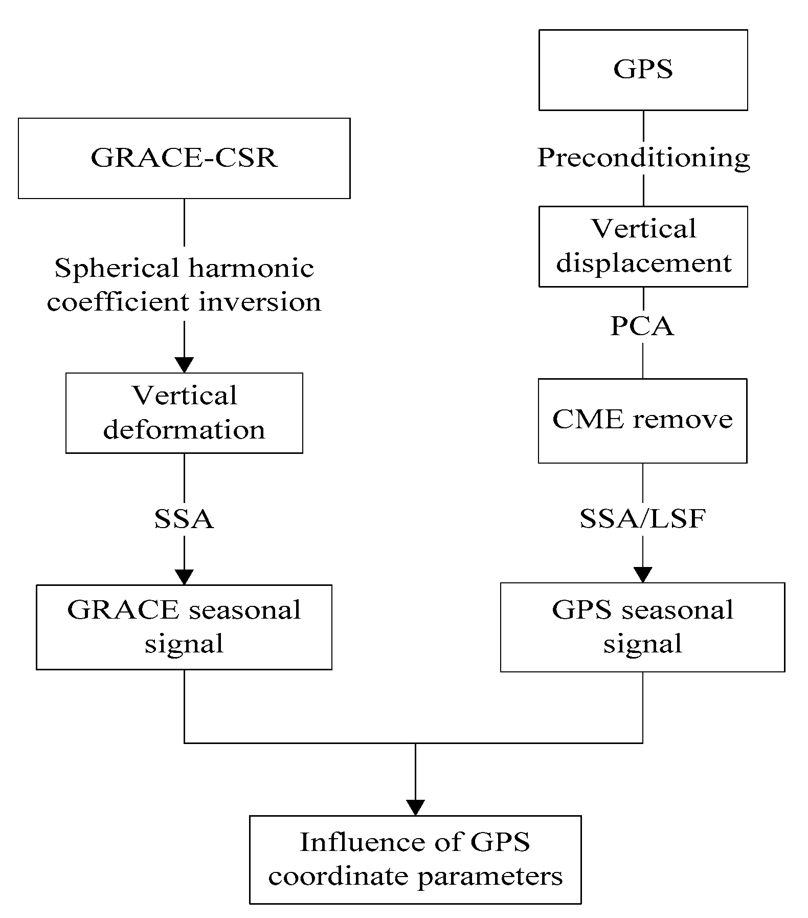
2. Materials and Methods
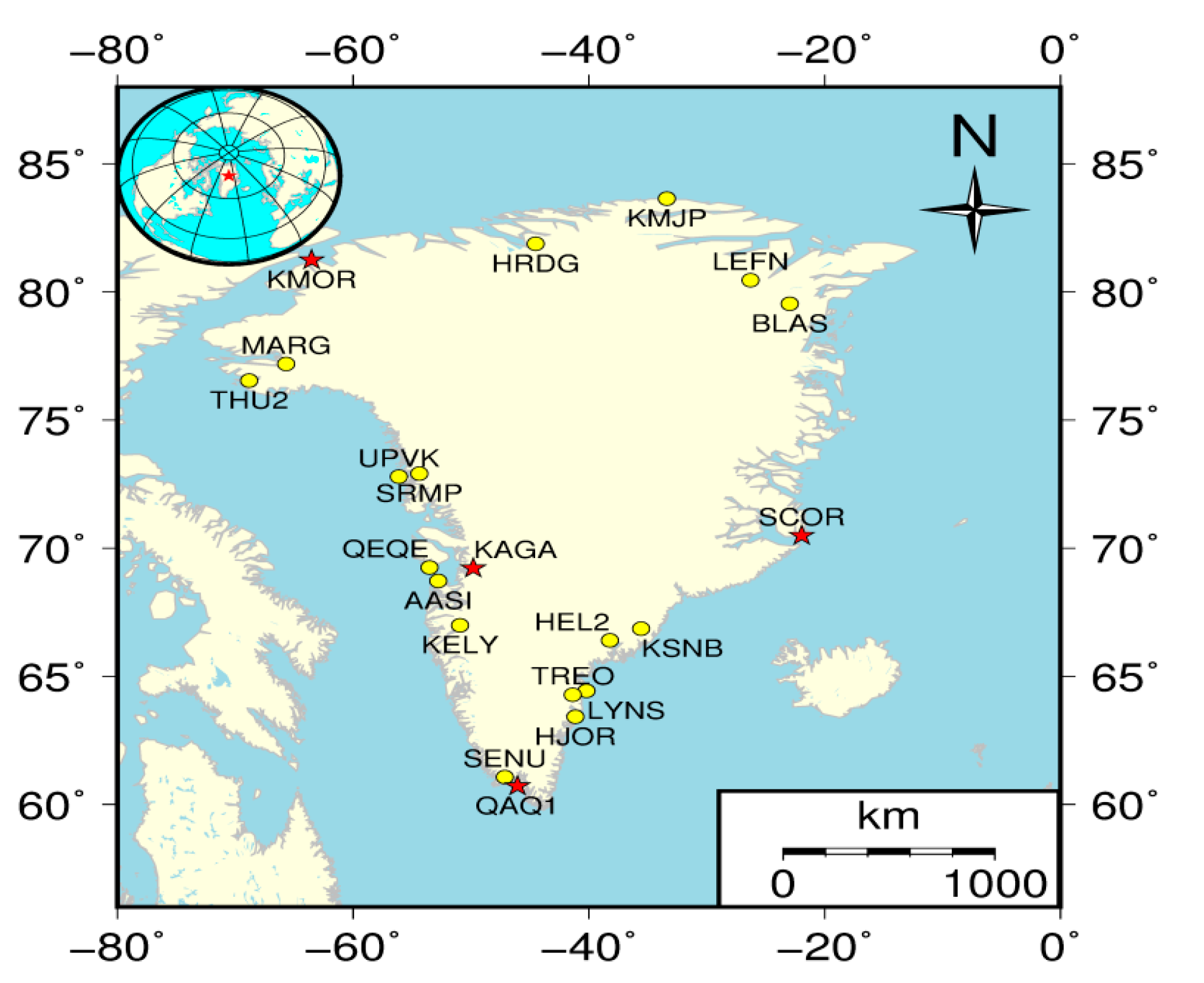
2.1. GPS Data

In order to overcome the problem of sparse distribution of IGS stations in Greenland, the POLENET organization effectively increased. Considering the accurate acquisition of the station velocity field, the station data need to be greater than 2.5 years [28], and have a low missing rate (no more than 10%). Therefore, this paper selects 21 observation stations (4 IGS stations) for research, with a time span from August 2008 to July 2016 (8 years), and the spatial distribution is shown in Figure 1.
In view of the problems such as step, gross error and missing data in the GPS station coordinate data, this paper has carried out a series of preprocessing measures, mainly including using the step time record data to correct the step term, the Triple Quartile Difference Method [29] to remove the isolated abnormal value, and combined interpolation method to fill in missing data [30]. In addition, we eliminated the linear trend of GPS station data according to the functional model adopted by Li et al. [31].

2.2. GRACE Data

The change of mass loads included atmosphere, and ocean and surface water of the earth, and will cause crustal elastic deformation. Studies have shown that the vertical surface deformation can be carried out through a set of spherical harmonic coefficients of the gravity field and loading Love numbers [11], and their spatial and temporal resolutions are month and 1° × 1°, written in Equation (1) as follows:
Δ h ( θ , λ ) = R l = 1 N max m = 1 l h l 1 + k l ( Δ C l m cos ( m λ ) + Δ S l m sin ( m λ ) ) P ˜ l m ( sin ( θ ) )
where   Δ h   θ , λ represents the vertical surface deformation, R is the Earth average radius (6371 km), S l m   a n d C l m   are the coefficients changes of the normalized complex spherical harmonic (Stokes’ coefficients), θ and λ are the latitude and longitude, P   ˜ ( sin θ represents the fully normalized Legendre function, Nmax is the gravity field model maximum coefficient, and   k   l   a n d   h   l are the L-order loading Love numbers provided by Farrell [32].
The data used are the GRACE RL06 spherical harmonic coefficients provided by the Center for Space Research (CSR) institution (ftp://podaac.jpl.nasa.gov/allData/grace/L2/CSR/RL06/) accessed on 12 September 2022, with the time span from August 2008 to July 2016. In the data preprocessing process, the variation value of spherical harmonic coefficients in each month is obtained by deducting the average gravity field model of all months. For the degree 1 terms, the evaluation of geocentric correction term (i.e., S11, C11 and C10) based on Sun et al. [33] are available here (https://podaac-tools.jpl.nasa.gov/drive/files/allData/grace/docs/TN-13_GEOC_CSR_RL06.txt) accessed on 12 September 2022, and the degree 2 coefficients were replaced from SLR [34] is available as TN14 (https://podaac-tools.jpl.nasa.gov/drive/files/allData/gracefo/docs/TN-14_C30_C20_GSFC_SLR.txt) accessed on 12 September 2022; Based on the experience of predecessors, the order of spherical harmonic coefficient was 60, and the higher order terms and correlation errors of spherical harmonic coefficients generated in the inversion process were eliminated by the combined form of Gaussian filtering (radius of 250 km) and P4M6 de-correlation filtering [35,36]. In the process of error processing, the forward-modeling method of Jin et al. [37] was used to solve the problem of signal leakage. Due to the influence of glacier equalization adjustment (GIA), the method provided by Geruo et al. [38] was used to solve the problem. In addition, since the acquired GPS vertical deformation data include the influence of non-tidal ocean and atmospheric loads, in order to maintain consistency, it is necessary to add the GAC product to the GRACE spherical harmonic solution.

2.3. Singular Spectrum Analysis

For seasonal periodic signal extraction of GPS coordinate time series, the least square-fitting method is usually used. The premise of this method is to assume that the phase and amplitude of the periodic signals are both fixed values, that is, sine cosine functions, which is not the case in reality.
The Singular Spectrum Analysis (SSA) method is formed based on the Karhumen-Loeve Orthogonal Decomposition Theory. This method can not only perform principal component analysis on one-dimensional time series, but also effectively identify and extract periodic signals without any prior information and non-sine cosine wave hypothetical conditions [39], so it is widely used in many fields such as meteorology, hydrology, and dynamics. For a given one-dimensional time series x = (x1, x2, …, xN), N is the length of the sequence. According to the window length L (1 ≤ LN/2), we calculate the trajectory matrix X for a given time series, expressed as follows:
X = x 1 x 2 x L x 2 x 3 x L + 1 x N L + 1 x N L + 2 x N
where X is the matrix with K rows and L columns, K = NL + 1. The covariance matrix C of the X matrix is solved as follows:
C = X X T
where XT is the transposition matrix of the X matrix. The eigenvalues λi ≥ 0 (1 ≤ iL) and eigenvectors of the matrix C are derived. The eigenvector Ek corresponding to λk is the empirical orthogonal function (EOF) [40]. The k-th principal component   a i k is expressed as follows:
a i k = j = 1 L x i + j E j k
where the range of i is 0 ≤ i ≤ N-L, and j is 1 ≤ jL.
Finally, the reconstruction component x i k can be composed Ek and a i k of the k-th [41], expressed as follows:
x i k =   1 i j = 1 i a i j k E j k                               f o r                                                         1     i     L 1 1 L j = 1 L a i j k E j k                                   f o r                     L     i     N L + 1   1 N i + 1 j = i N + L L a i j k E j k               f o r               N L +   2     i     N
According to Plaut and Vautar [42], the following criteria can be used to identify periodic harmonic oscillation signals: (1) a pair of consecutive near-equal eigenvalues; (2) the constructed RCs are nearly orthogonal; (3) the associated EOFs are near-periodic.

2.4. Evaluation Indices

2.4.1. Weighted Root Mean Square (WRMS)

In order to explore the relationship between GPS coordinates and GRACE load deformation, Van Dam et al. [11] proposed a method that a percentage change of the WRMS of GPS station vertical displacement time series before and after deducting GRACE load deformation to measure the correlation, and its expression is as follows:
W R M S r e d u c t i o n = W R M S G P S W R M S G P S G R A C E W R M S G P S × 100
where WRMSGPS represents the WRMS of the GPS vertical displacement after linear detrend, and WRMSGPS−GRACE shows the WRMS of the GPS vertical displacement after removing the GRACE load deformation. Ideally, when the two are identical, the GPS vertical displacement WRMS reduction ratio is 1. When WRMSGPS−GRACE is smaller than WRMSGPS, it indicates that the GPS vertical displacement accuracy is improved after the GRACE load deformation correction. Additionally, the smaller the former, the better the correction effect. When WRMSGPS−GRACE is greater than WRMSGPS, it indicates that the GPS vertical displacement accuracy is reduced after the GRACE load deformation correction, and the larger the former, the worse the correction effect.

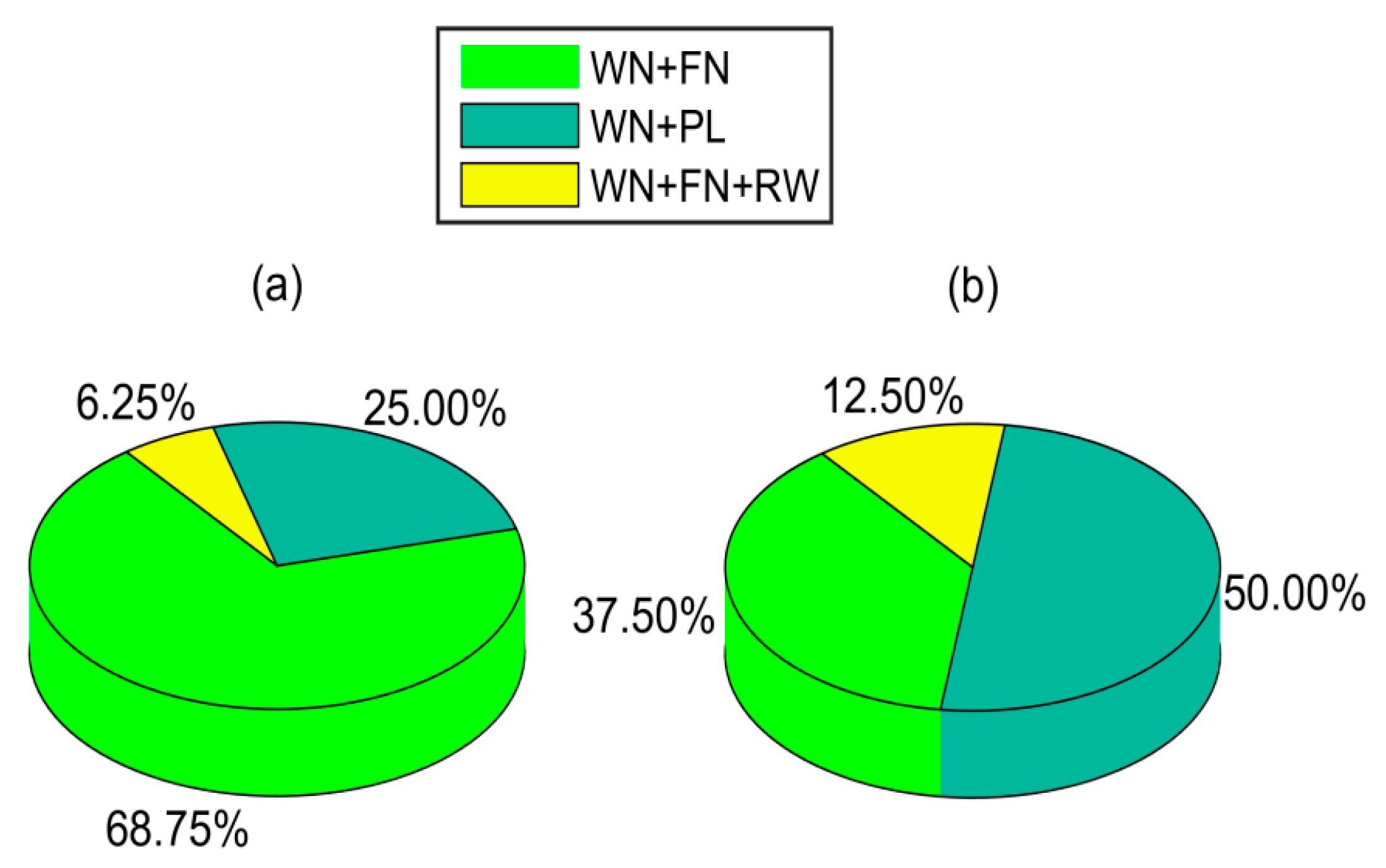
2.4.2. Optimal Noise Model

Theoretically, the noise characteristics of GPS station coordinate data should be pure white noise, which is not the case in reality. On the basis of maximum likelihood estimation (MLE), the Bayesian Information Criteria (BIC) and Akaike Information Criteria (AIC) methods can be used to determine the optimal model [43] to obtain a more reliable noise model to estimate the station coordinate parameters. The basic principle is as follows:
A I C = 2 k + 2 ln ( L )
B I C = k ln ( N ) + 2 ln ( L )
where k represents the model parameters number, N represents the data number, L represents the maximum likelihood function. When the results of AIC and BIC are consistent, the smaller model is selected as the optimal noise model. If the AIC and BIC results are inconsistent, the one with the smallest AIC value is preferred as the optimal noise model [27].

2.4.3. Amplitude Contribution

In order to intuitively express the influence of GRACE load deformation on the GPS station seasonal term (annual + semiannual), the Amplitude Contribution Rate (ACR) can be used to quantitatively describe its correction effect [27]:
A C R = ( 1 ( A c o r r e c t e d A o r i g i n a l ) ) × 100 %
In the formula, Aoriginal and Acorrected, respectively, are the seasonal amplitude before and after the GRACE load deformation correction station coordinates. When ACR > 0, it means the seasonal amplitude of the station after correction decreases. When the ACR value is closer to 1, this indicates that the seasonal amplitude reduction in the station after correction is more obvious. When ACR = 1, it means that the seasonal amplitude of the station after correction is 0.
In a word, our methodology can be summarized as follows and is shown in the flow diagram of Figure 2. Firstly, we analyzed the common mode errors of GPS stations and effectively eliminated them (Section 3.1). Secondly, the seasonal signals of GPS coordinates extracted by SSA and LSF methods are compared and analyzed (Section 3.2). On this basis, the seasonal signals of GRACE vertical deformation data are extracted by the SSA method and compared with GPS data (Section 3.3). Finally, the influence of seasonal load deformation of GRACE on coordinate parameters (noise characteristics, linear velocity, seasonal amplitude, etc.) of GPS stations is explored (Section 3.4).

3. Results and Discussions

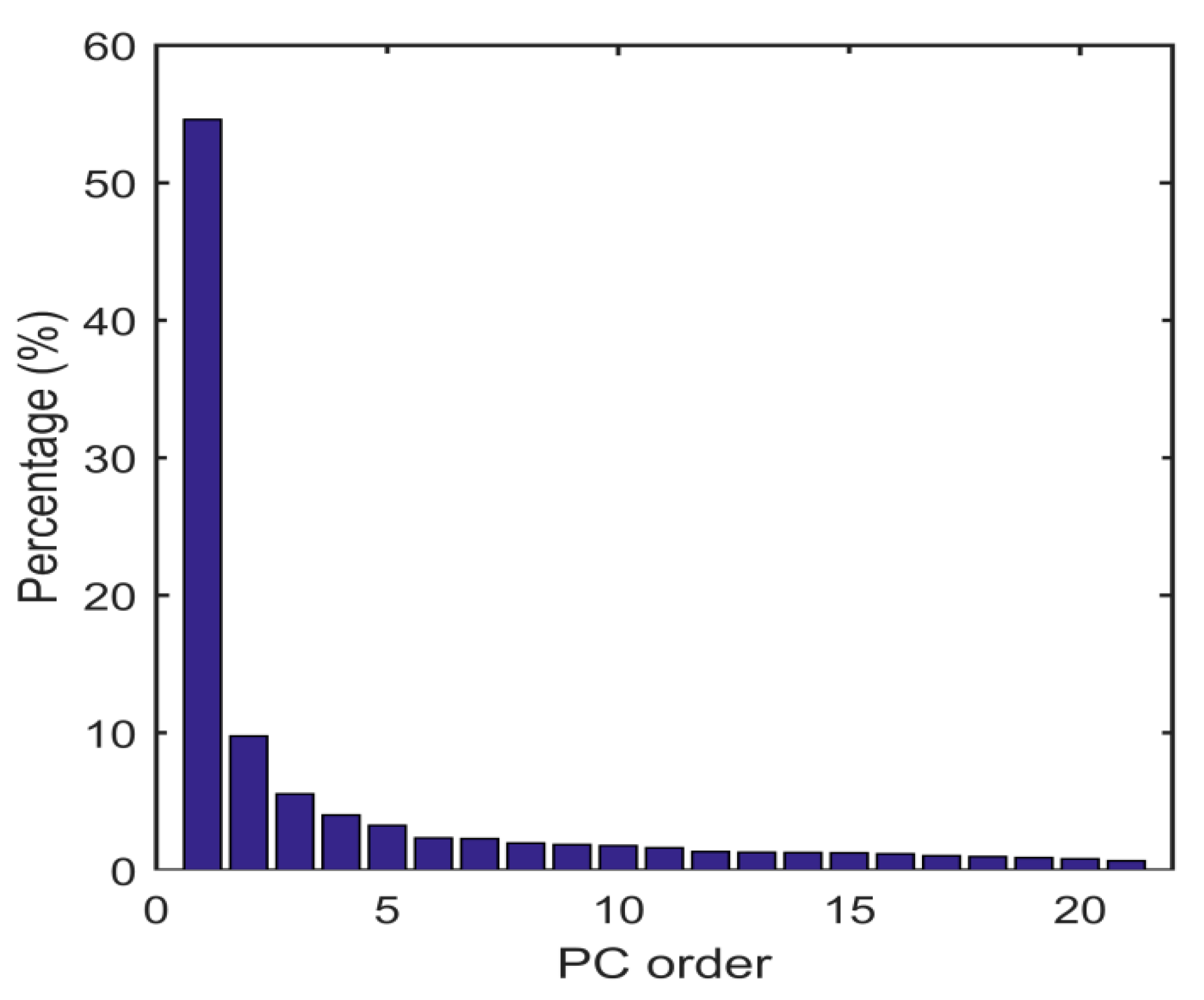
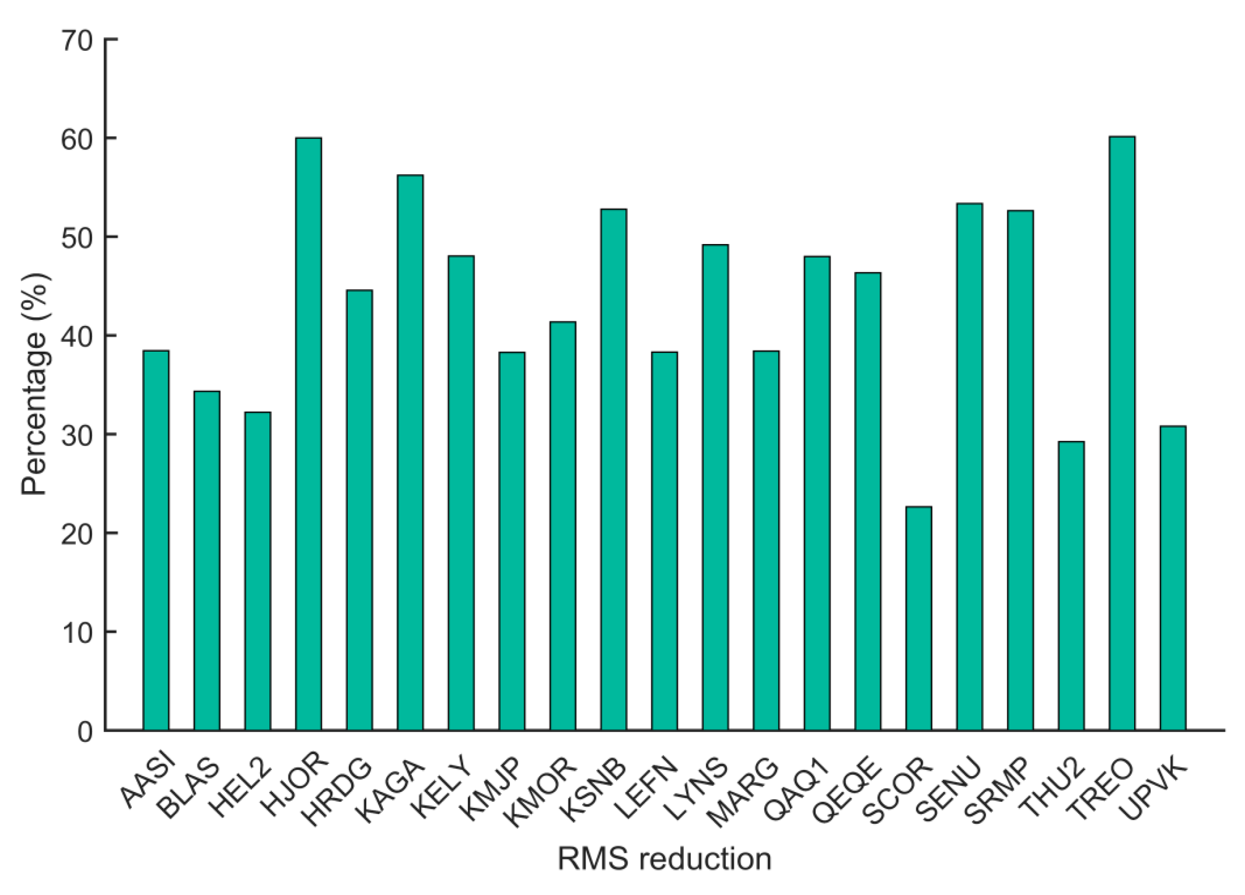
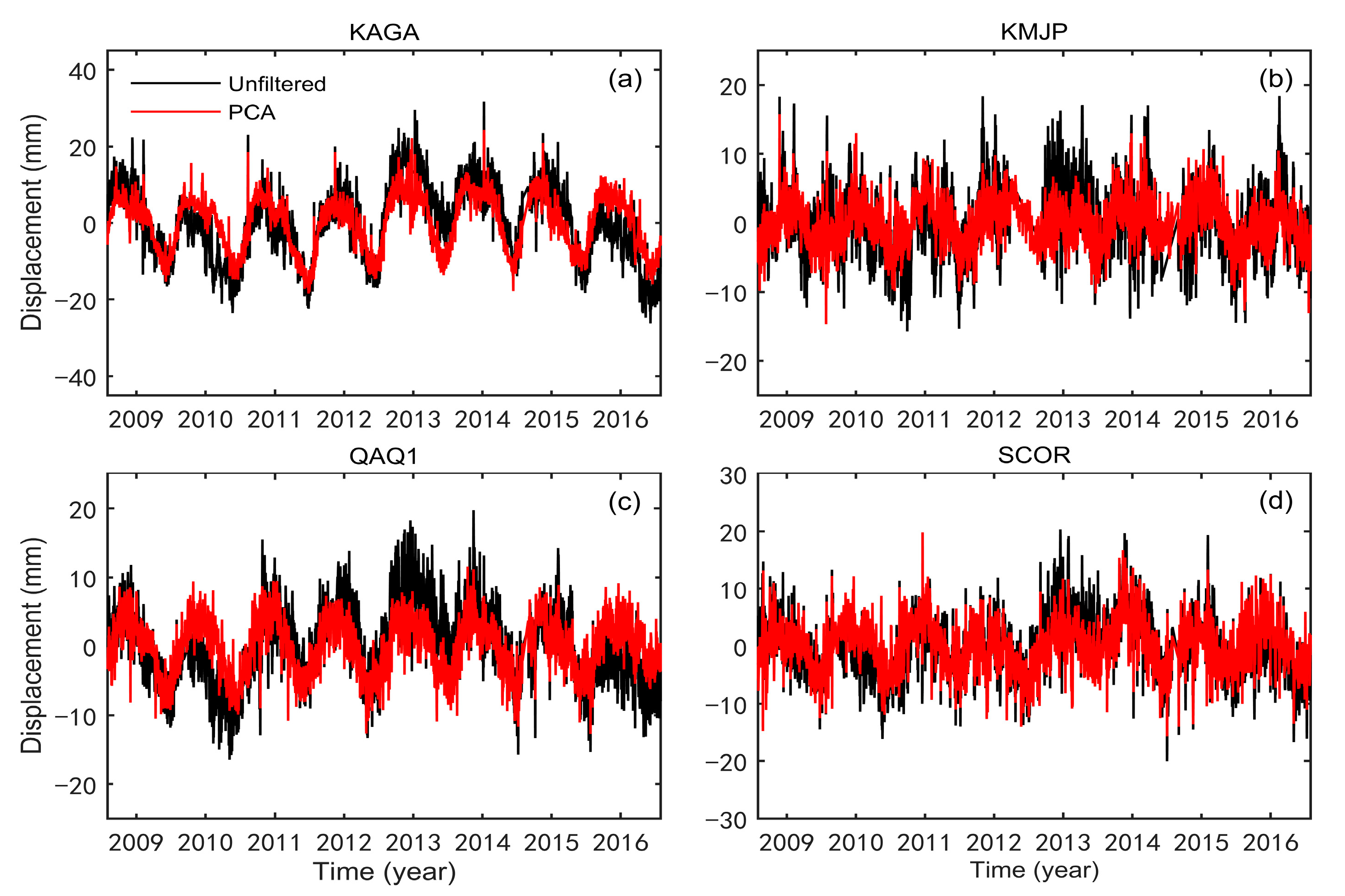
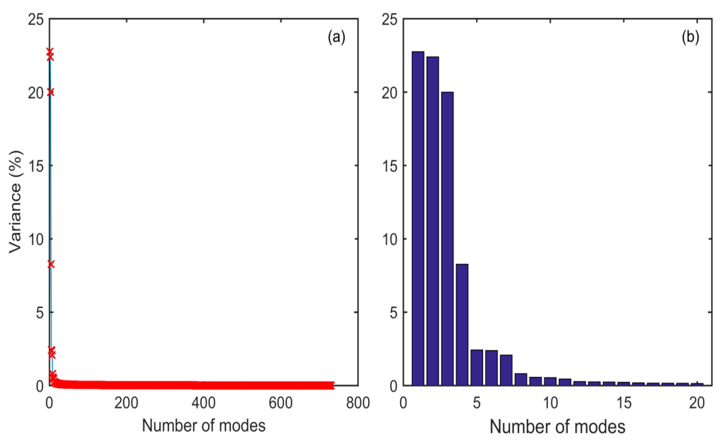
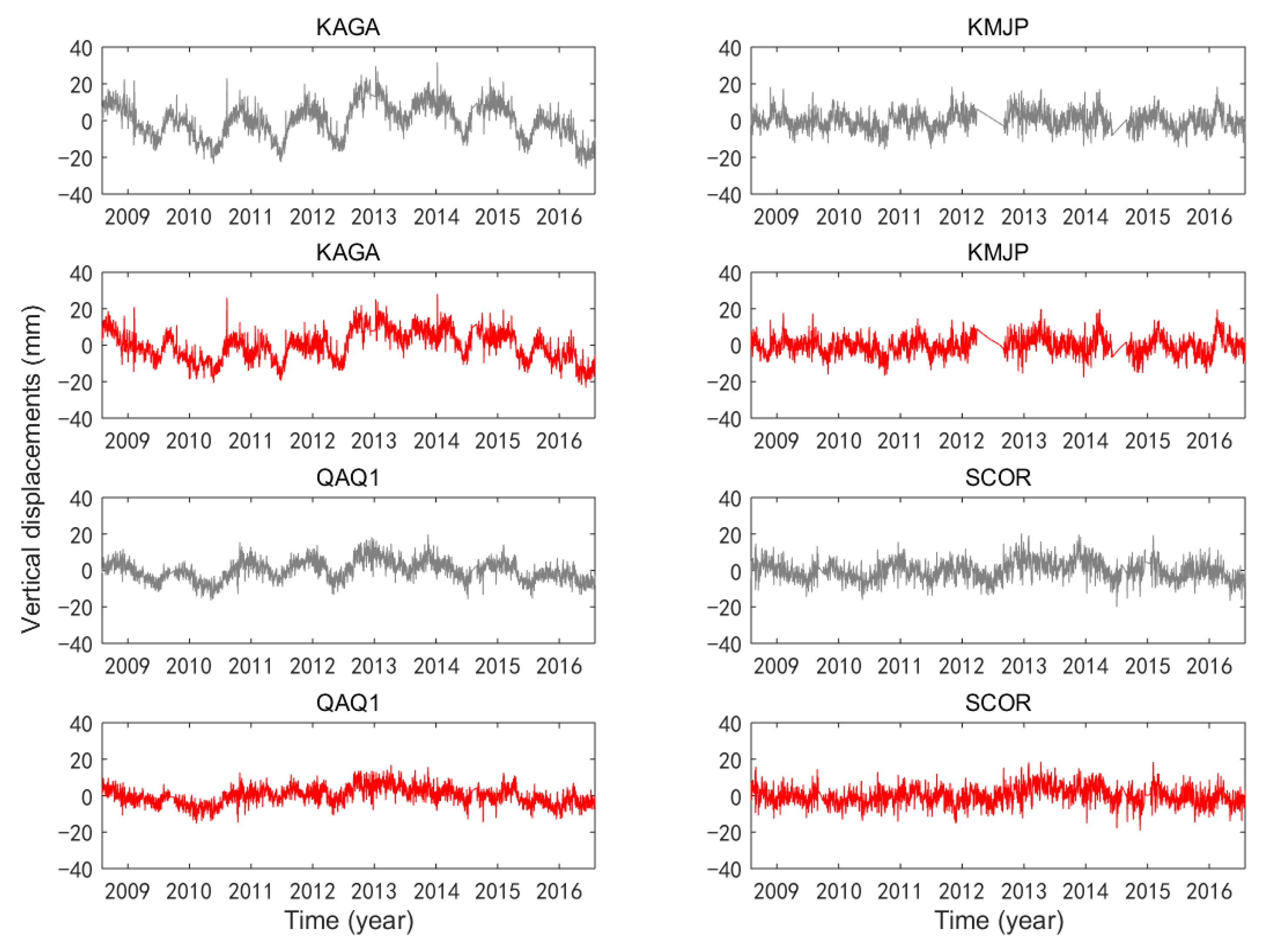
3.1. Common Model Error Analysis of GPS Station Coordinates

In order to improve the GPS station’s coordinate accuracy, the Common Modulus Error (CME) needs to be effectively eliminated. Bian et al. [23] found that the PCA method can better eliminate CME and improve coordinate accuracy in Greenland stations than KLE and Stacking. Therefore, this paper uses the PCA method for filtering. For more details, please refer to the literature of Bian et al. [23].
When determining the principal components constituted by CME, the normalized spatial response and eigenvalues are considered for each principal component mode, respectively. Figure 3 describe the proportion of normalized spatial responses and eigenvalues of the first 21 components extracted. It is found that the cumulative contribution rate of the first three principal components in the vertical direction obtained by PCA filtering is 69.91%, and the corresponding percentage of eigenvalues is greater than 1%. Table 1 shows the normalized spatial responses of the first four principal components of the stations (each eigenvector divided by its absolute maximum element). It can be seen that the normalized spatial responses of most stations in the first three principal components exceed 0.25, while at least half of the fourth principal components do not exceed 0.25, and only the first three principal components meet the so-called common mode criterion of Dong et al. [44] (For more than half of the stations, the standardized spatial response is greater than 25%, and the proportion of corresponding eigenvalue is greater than 1%.). To sum up, the first three principal components are selected as this region CME.
Furthermore, to quantify the impact of CME elimination on station coordinates, Figure 4 shows the RMS value changes of GPS station residual data before and after CME filtering, and can be seen that the RMS of the vertical coordinate residual of each station has decreased significantly. The minimum reduction is 22.64%, the maximum reduction is 60.13%, and the average value is 43.58%, which indicates that the CME in the station coordinates is well removed after filtering [45].
Furthermore, Figure 5 shows the coordinate time series changes in the vertical direction of four uniformly distributed GPS stations without filtering and after PCA filtering. It can be seen from the figure that the coordinate time series after filtering (red line) is more convergent than the pre-filtered sequence (black line), indicating that the PCA filtering is capable of effectively reducing the uncertainty of GPS station coordinate.

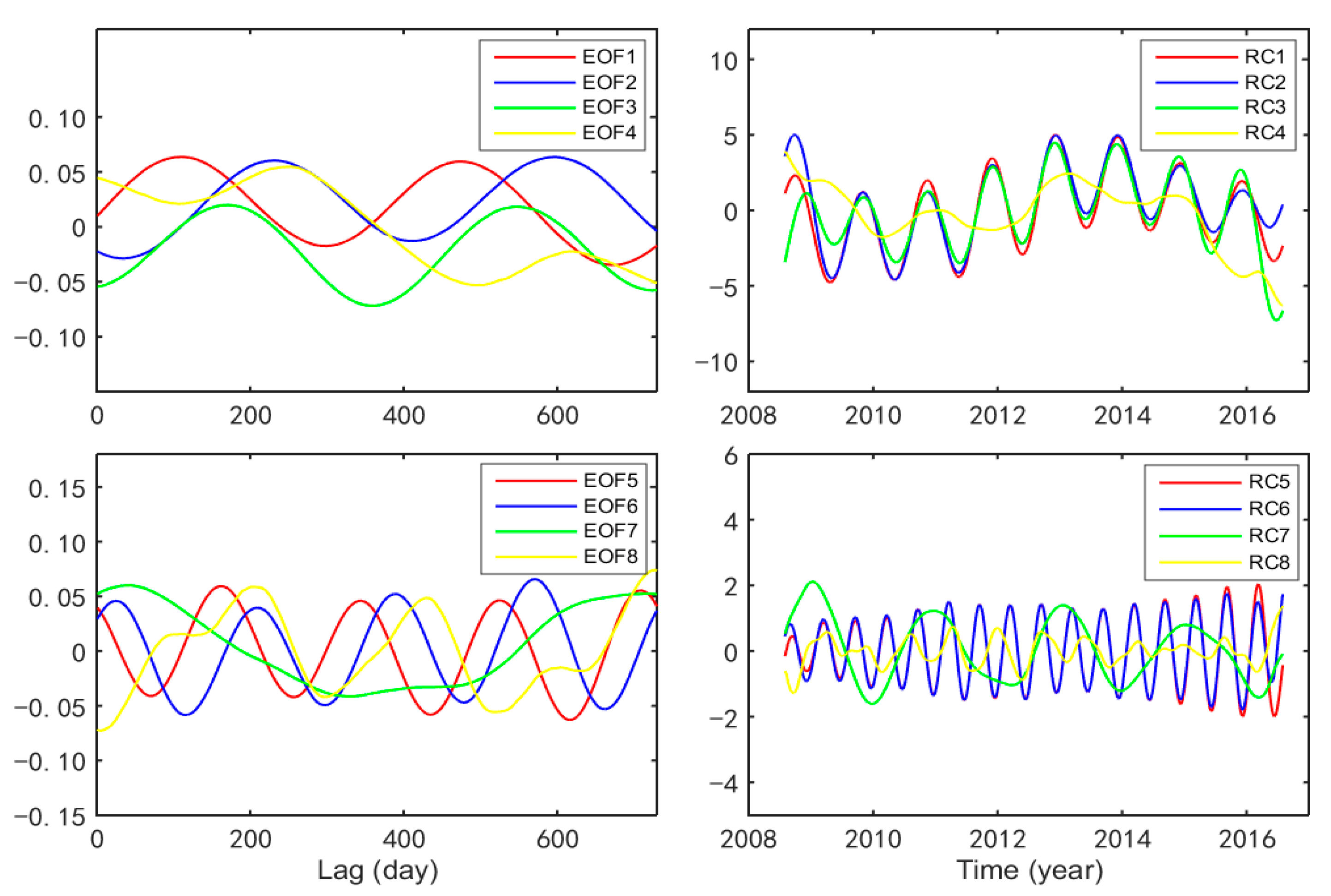
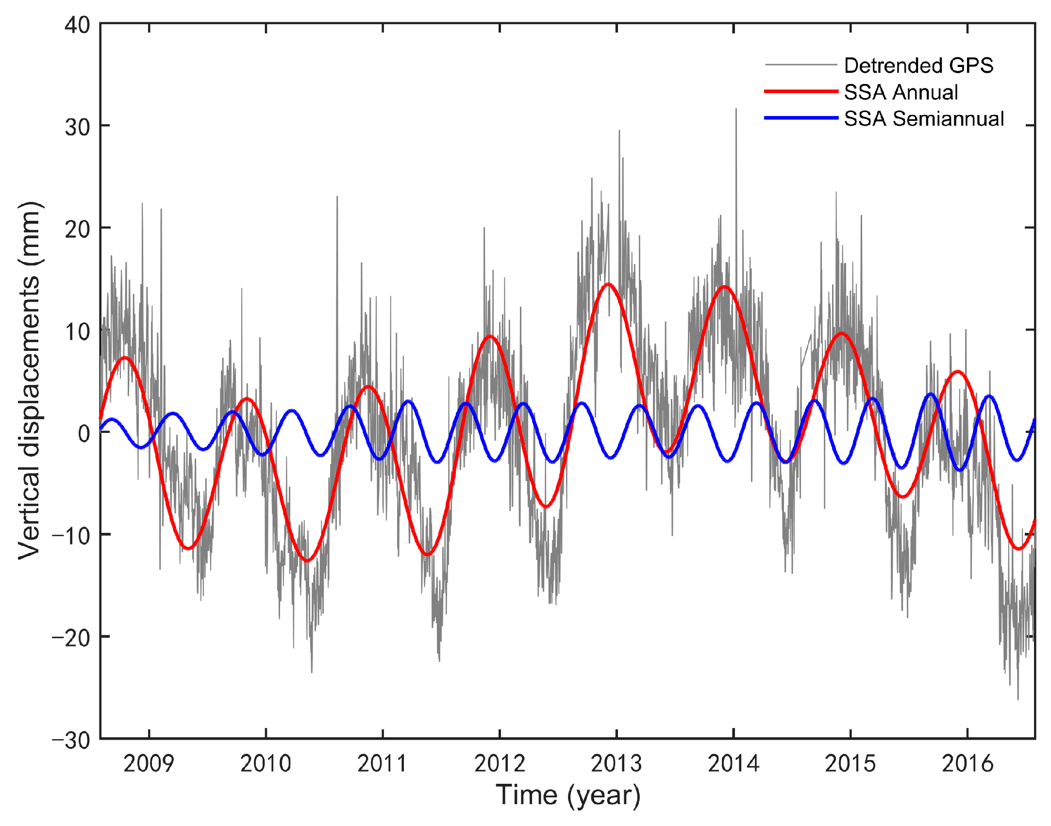
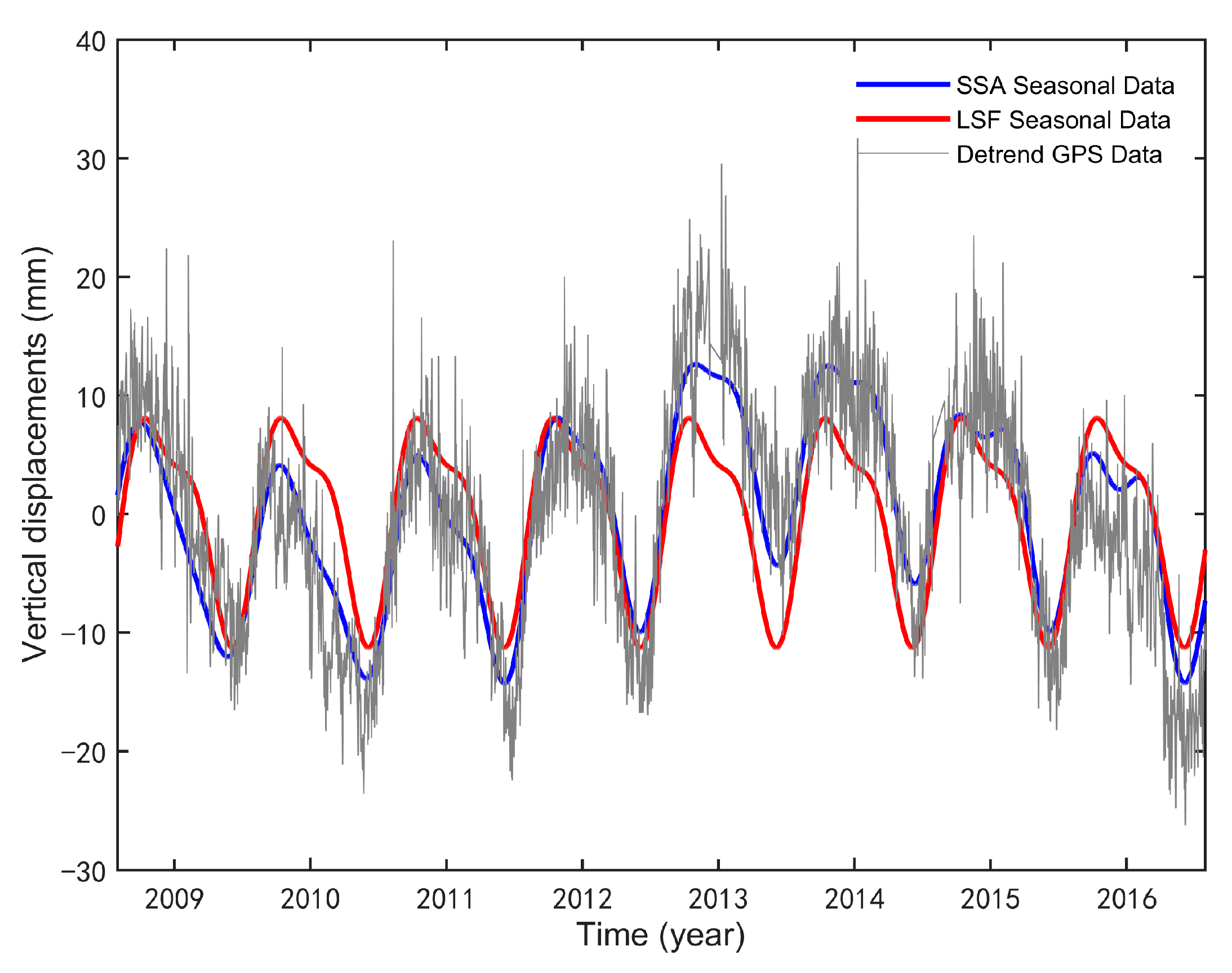
3.2. Seasonal Signal Extraction of GPS Station Coordinates

On this basis, in order to better compare and analyze the seasonal vertical deformation between GRACE and GPS, it is necessary to effectively extract seasonal signals. Chen et al. [46] studied the selection of lag window size in data simulation by the SSA method, and found that the 2 or 3 years was particularly suitable for seasonal signal extraction. Based on the research of some scholars [47,48], a 2-year lag window was selected to extract the seasonal periodic signal of GPS station coordinates. Taking the KAGA station as an example, and the same processing is carried out for other stations. Figure 6 and Figure 7 show the contribution rate of the first 20 time modes, and the variance of the first four pairs of temporal principal components (EOFs) and temporal principal components (RCs), respectively.
According to the criteria of Plaut and Vautar [42], the 1st to 3rd reconstruction components (RCs) are identified as vertical deformation annual signals, and the 5th to 6th reconstruction components (RCs) are identified as vertical deformation semiannual signals. Among them, the variance of the seasonal (annual + semi − annual) signals explained 49.97% of the total. Finally, the seasonal periodic signals of the station are reconstructed based on the above reconstructed components (RCs), as is shown in Figure 8.
To further evaluate the performance of SSA method for extracting vertical periodic signals from GPS stations, the station seasonal variation signals extracted by the SSA and the least squares fitting (LSF) methods were compared and analyzed, as shown in Figure 9. It can be seen that both SSA and LSF methods can effectively extract seasonal periodic signals. However, when its amplitude changes, SSA has the ability to obtain the peak value of the time-varying periodic signal, while the amplitude of the LSF extracted periodic signal is always fixed, and the seasonal signal obtained by the SSA method is closer to the GPS real signal, indicating that the SSA method is superior to LSF in extracting seasonal signal.

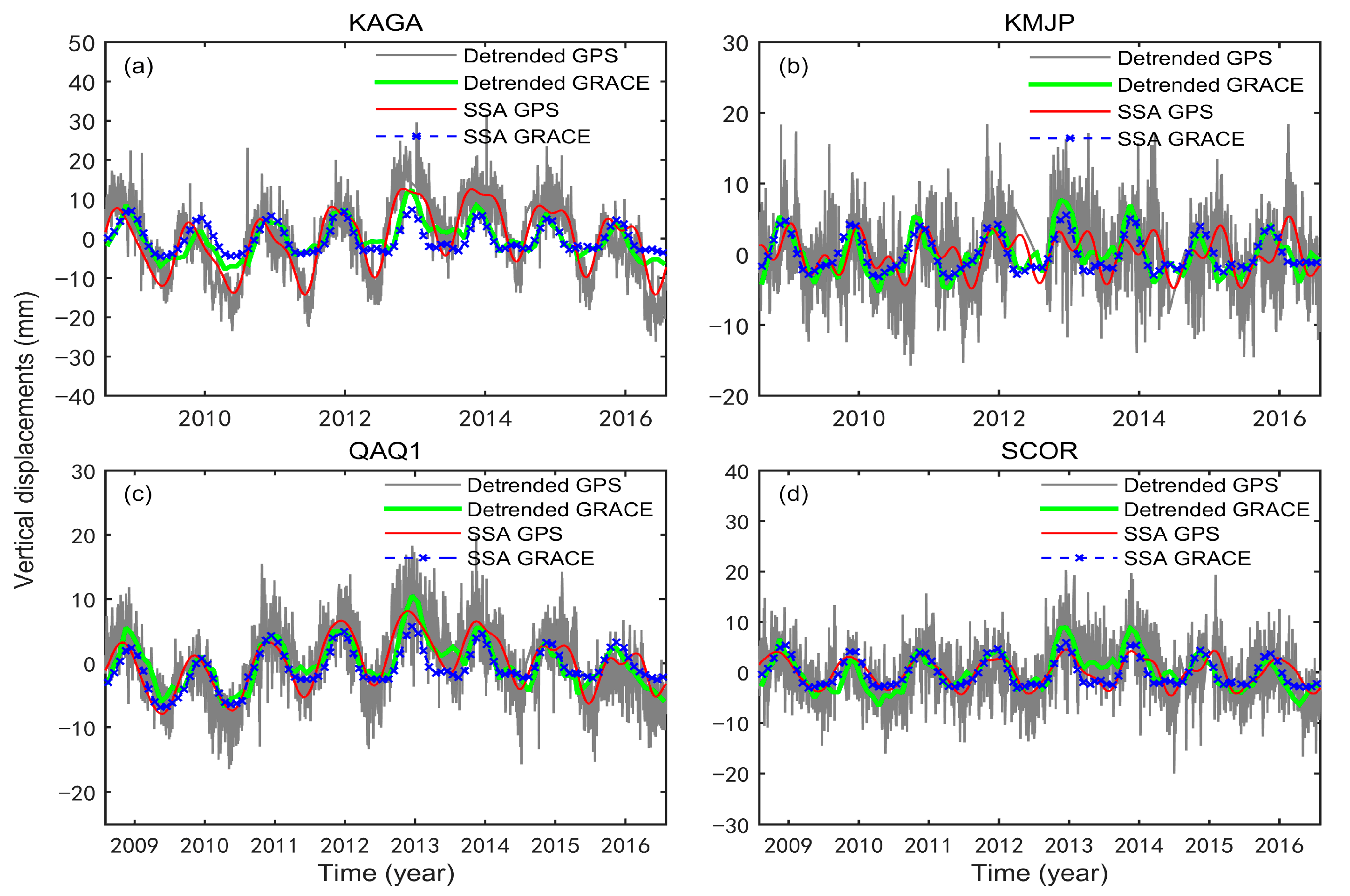
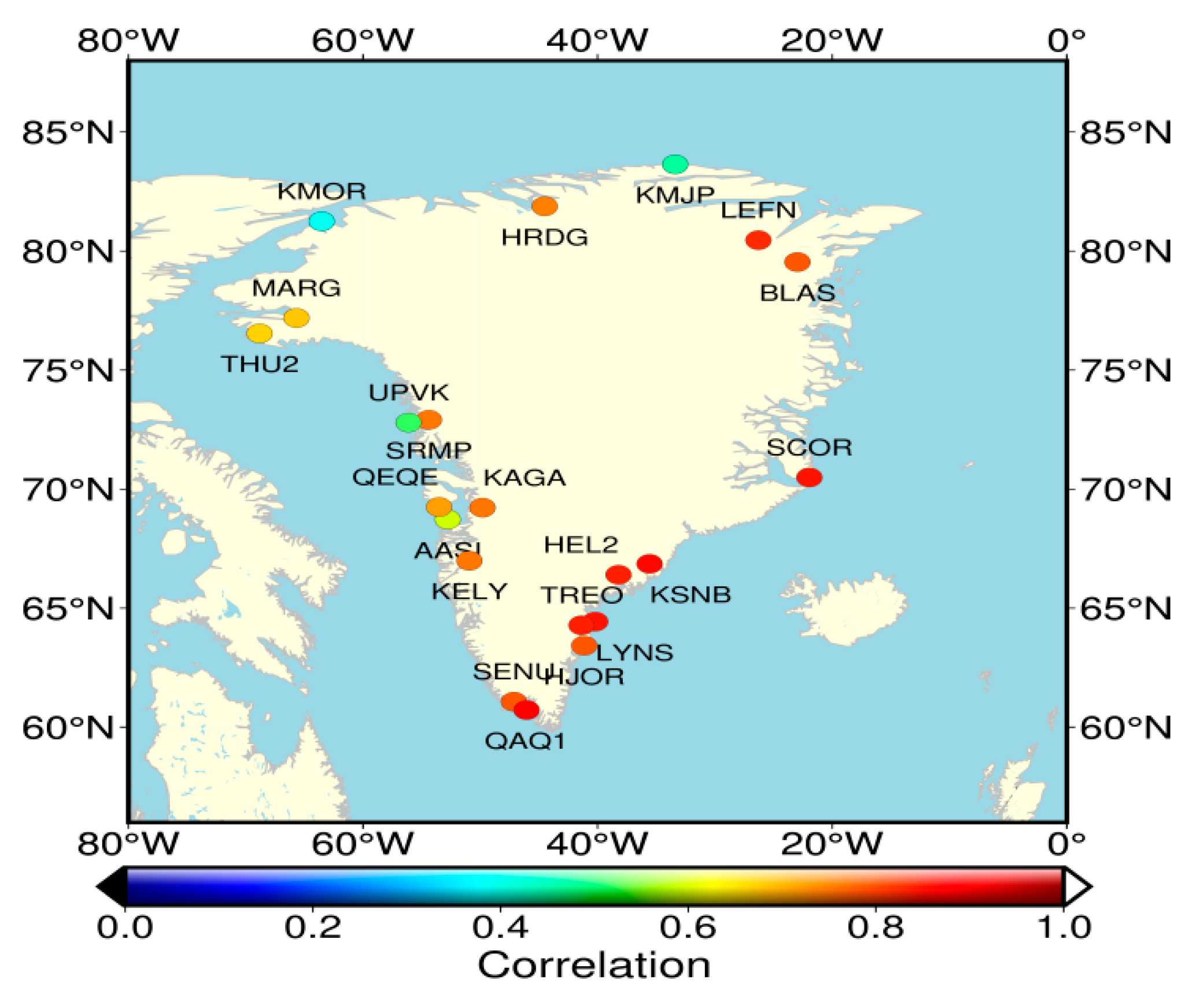
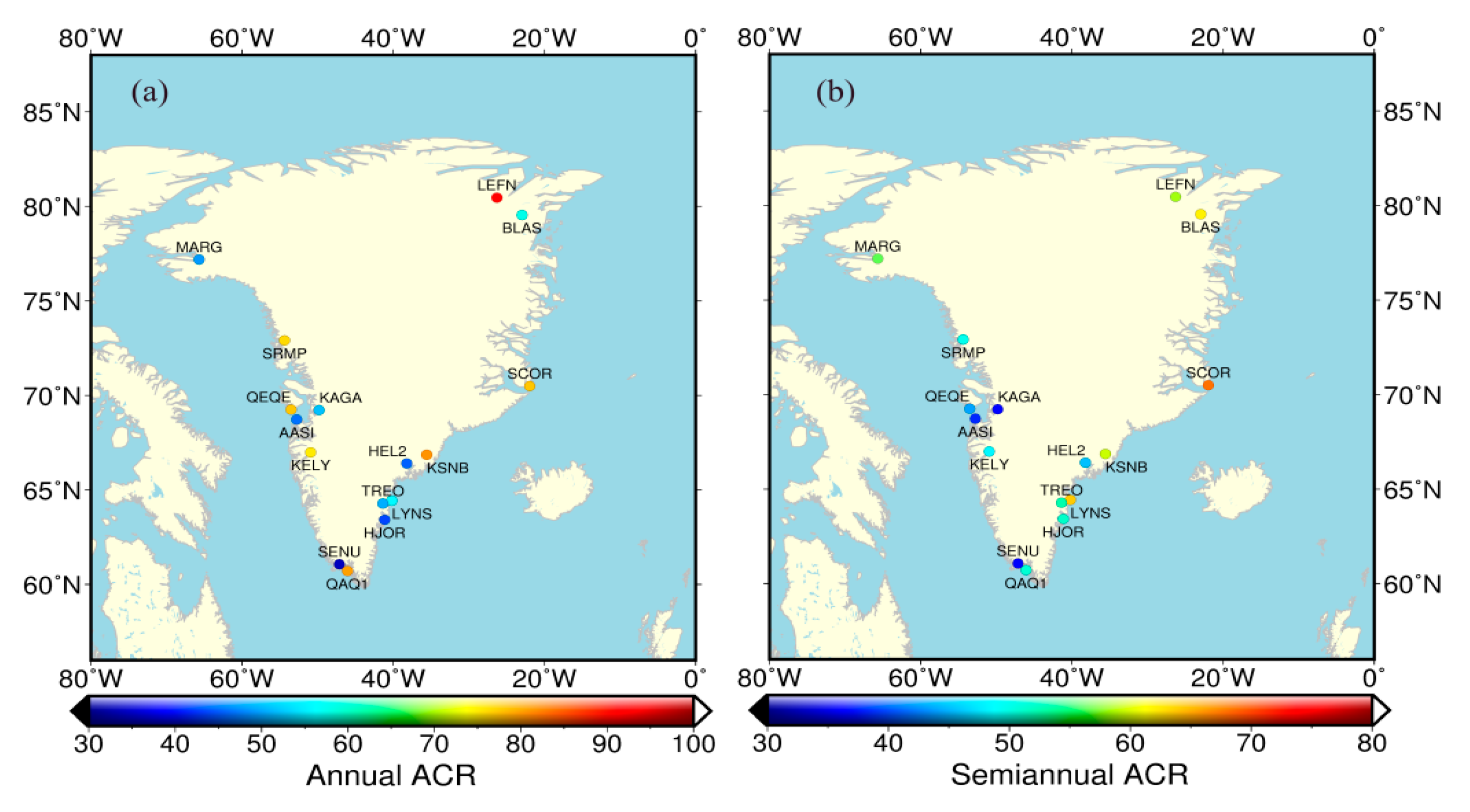
3.3. Comparative Analysis of GRACE and GPS Seasonal Vertical Deformation

In order to explore whether the geophysical signal process can explain the seasonal periodic movement of GPS stations, the seasonal periodic signals of the vertical displacement and GRACE mass load deformation of each station were obtained by the SSA method, and the amplitude and phase were compared and analyzed, as shown in Figure 10. Figure 10 shows that the QAQ1 and SCOR stations located in the south and east of Greenland, respectively, have obvious consistency with the seasonal vertical deformation signals of GRACE and GPS, in that not only the amplitudes are the same, but the phases are also basically the same, indicating that the seasonal vertical displacement of GPS stations mainly comes from the mass load deformation [19,21]. The KAGA stations in the west are basically consistent in phase, but the amplitude is smaller than the station coordinates, indicating that the mass load deformation may only be partly caused by the nonlinear motion of the GPS stations. At the KMJP station, there are obvious inconsistencies in the amplitude and phase, indicating that the seasonal load effect observed by GRACE cannot explain the seasonal term of the vertical displacement of the station. In addition, from the analysis of the detrended change angle of GRACE and GPS data, it is found that the amplitude and phase relationship between them also have the above-mentioned situations and are consistent. For the remaining station data, the same processing is carried out in this paper.
From the correlation, we explored whether the seasonal deformation of GRACE and GPS are periodic vibrations caused by the same physical factors, and the correlation coefficient between them was calculated using the Pearson correlation, as shown in Figure 11. Figure 11 shows that the vertical displacement of GPS stations in Greenland is positively correlated with the GRACE mass load deformation, and the overall correlation average is 0.73, which indicates that there is a strong correlation. Among them, the correlation of 67% stations is around 0.8, indicating that the seasonal signals of GPS vertical displacement may mainly come from the mass load deformation. However, there are also some stations with weak correlation, among which the correlation coefficients of the northern stations (KMJP and KMOR stations) are below 0.5, which is different from the spatial differences in other regions [19,20,21].
The relationship between GPS and GRACE seasonal vertical deformation was further explored, and percentage change of WRMS at each station was calculated separately, as shown in Figure 12. Figure 12 shows that after the seasonal displacement of GPS stations is corrected by the seasonal load deformation of GRACE, the WRMS values of most stations become smaller, and some stations also increase. Among them, the maximum change is a decrease of 55.20% (QAQ1 station), the minimum value is −22.69% (KMJP station), and the average value is 25.38% with the obvious differences, which may be related to the complex changes of vertical motion in Greenland. For the QAQ1 and SCOR stations in the south and east, the WRMS reduction of the seasonal vertical deformation is 55.20% and 42.72%, respectively, indicating that it is feasible to use GRACE seasonal load deformation to correct the seasonal displacement of the GPS stations, and the effect is very obvious. However, the WRMS of the KAGA station in the east decreased by 32.29%, and the correction effect is relatively insignificant. The stations in the north (HRDG, KMJP, and KMOR stations) even showed increased WRMS, with values of −15.29%, −22.69%, and −4.78%, respectively, indicating that these stations could not be effectively corrected. In general, the seasonal variation of most GPS stations is mainly manifested as GRACE seasonal load deformation, and individual stations cannot reflect it effectively.
To more intuitively express the influence of the seasonal changes in GPS station coordinates, Figure 13 shows the selected GPS coordinate residual time series after removing the GRACE seasonal vertical load deformation. Among them, QAQ1 and SCOR stations hardly found any seasonal signals, indicating that the use of GRACE can effectively eliminate seasonal signals in GPS data. The KAGA station has some seasonal signals, indicating that the elimination effect is not good. However, the seasonal signal of KMJP station become more obvious, indicating that it cannot be eliminated. In conclusion, it can be found that the conclusion obtained from the station coordinates residual is consistent with the WRMS reduction ratio of the seasonal signal of GPS data corrected by GRACE.

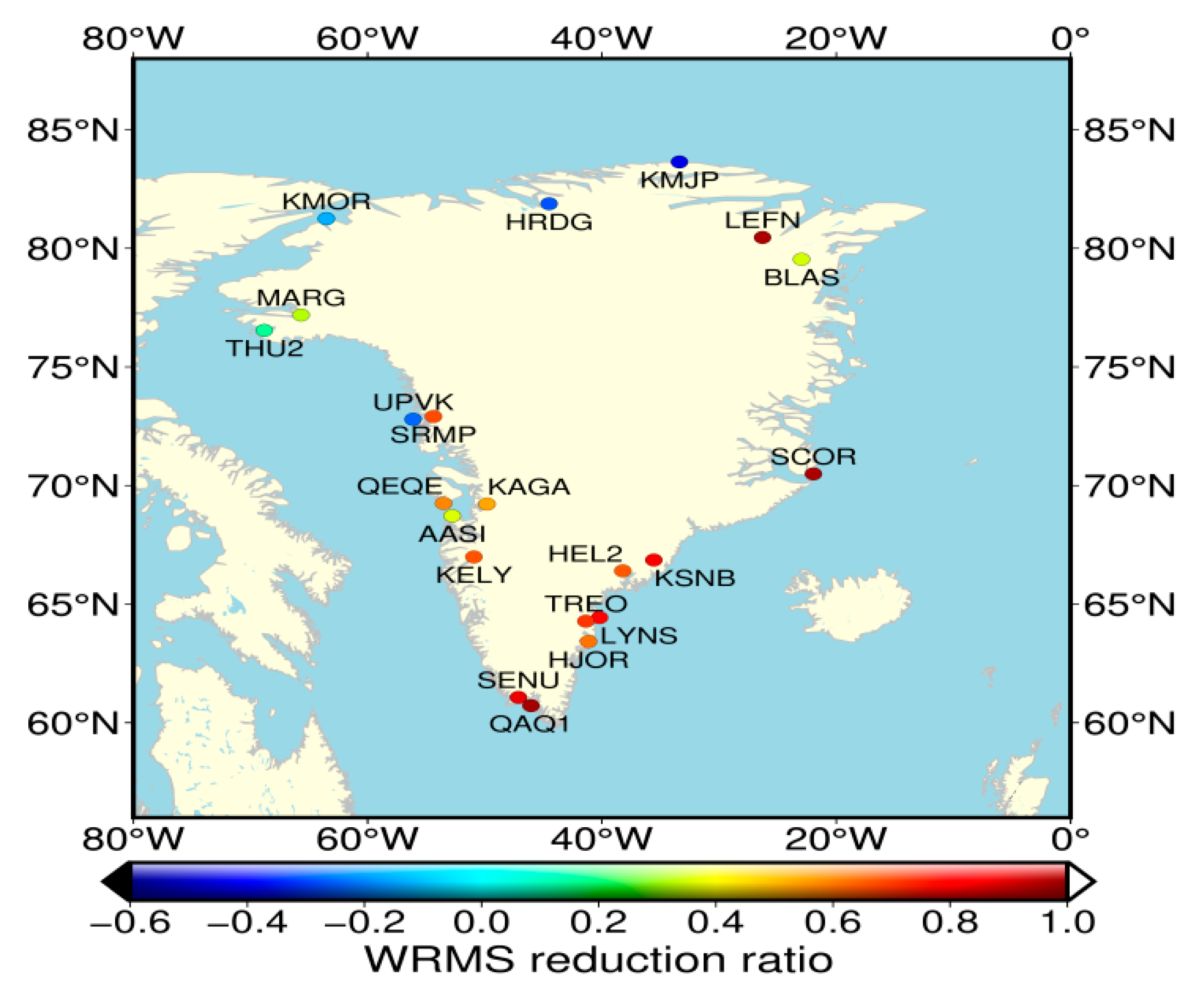
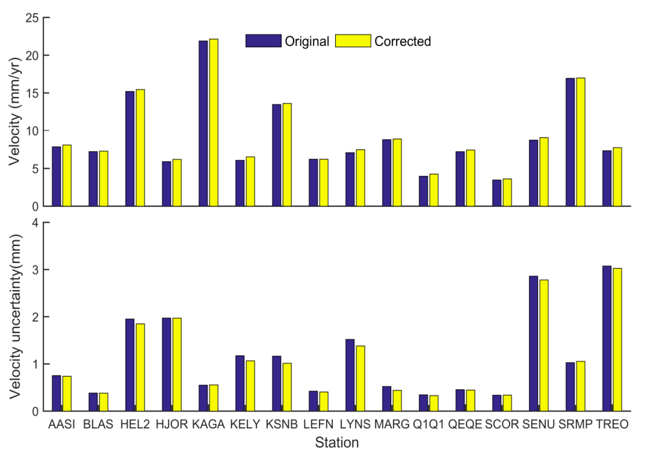
3.4. Influence of GRACE Seasonal Load Deformation on GPS Station Coordinates

On the basis of the above research, the influence of GRACE seasonal load deformation on the GPS station coordinate parameters is further analyzed, mainly including noise characteristics, linear velocity and uncertainty, and seasonal amplitude amplitude change.
In order to analyze the influence of GRACE seasonal load deformation on the noise of GPS stations in the study area, the noise models variation of the station coordinate before and after load correction were studied, based on four common combination models: white noise + power law noise (WN + PL), white noise + flicker noise (WN + FN), power law noise + random walk noise (PL + RW), and white noise + flicker noise + random (WN + FN + RW). The noise analysis before and after the GRACE load deformation is removed for each reference station and performed by CATS software, and the AIC and BIC indicators are used to identify the optimal noise model, as shown in Table 2.
At the same time, the optimal noise model changes before and after GPS station coordinates are corrected by the GRACE load deformation are given, as shown in Figure 14. It can be seen from Figure 14 that the proportion of WN + FN model decreased from 68.75 to 37.50%, and the WN + FN + RW model increased from 6.25 to 12.50%, while the FN + RW model is always 0, and the WN + PL model increased from 25.00 to 50.00%. Therefore, the optimal noise model in the station seasonal term is mainly WN + FN, and there are also some RW models. The above conclusions are different from the noise model of GPS stations on the Antarctic Peninsula studied by Li et al. [24], indicating that seasonal deformation of GRACE mass loading has different effects on the GPS stations coordinates in different geographical locations.
Based on the above optimal noise model, the CATS software was used to estimate the velocity and uncertainty changes before and after the GPS station coordinates were corrected by the GRACE seasonal mass load, as shown in Figure 15. It can be seen that the station velocity does not change much before and after removing the GRACE seasonal load deformation. The velocity of each station varies between 0.01 and 0.46 mm/yr, with an average value of 0.23 mm/yr, and all stations show an increase. The uncertainty ranges from −0.03 to 0.15 mm/yr, with an average value of 0.05 mm/yr, which basically shows a decrease, except for individual stations of KAGA and SRMP. The above shows that the influence of the GRACE seasonal load deformation on the station vertical velocity reaches the order of 0.01 mm/yr, and the uncertainty of the station velocity is basically reduced, which is very important for the construction of millimeter level and higher precision earth reference frame.
In addition, in order to intuitively express the influence of GRACE seasonal load deformation on the amplitude of GPS stations seasonal term (annual + semi−annual), the ACR was used to quantitatively describe its correction effect. Figure 16 shows that the annual and semiannual amplitudes of the station decrease after the GRACE seasonal load deformation correction. Among them, the ACR value of the annual amplitude in Figure 16a is between 33.95% and 90.97%, and the average value is 62.11%, indicating that the maximum contribution rate of GRACE seasonal load deformation to the vertical annual amplitude of the station reaches 90.97%, and the average contribution rate is 62.11%. Meanwhile, Figure 16b shows the semiannual amplitude change after GRACE seasonal load deformation correction. It is found that the relative annual amplitude change is small, with the ACR values ranging from 35.87 to 68.26%, with an average value of 51.33%. To sum up, the annual and semiannual signals fluctuation of GPS station coordinates are weakened after the GRACE seasonal load deformation correction, which is beneficial from the point of view of signal denoising.

4. Discussions

4.1. Cause for Vertical Seasonal Changes Affecting Differences

This paper discusses the relationship between GRACE seasonal load deformation and GPS station coordinate data from the aspects of time series amplitude and phase, correlation degree, and WRMS change. Among them, Section 3.3 of the paper finds that the seasonal signals of most stations in eastern and southern Greenland are mainly from environmental load deformation, and the western region can explain a few reasons, while the northern region cannot. For example, QAQ1 and SCOR stations, located in the east and south, KAGA stations in the west, and HRDG, KMJP, and KMOR stations in the north. The reason for the above may be that some scholars found that the GPS stations seasonal changes were caused by the combined effects of surface mass load deformation, imperfect GPS processing models (troposphere, atmospheric tide, and ionospheric delay, etc.), and geophysical model related factors (temperature), among which the hydrological load deformation in surface mass load deformation has a large difference in different regions [4,7,49]. For the analysis of the above influencing factors, due to the lack of certain data and equipment, it is difficult to conduct a comprehensive and detailed study, especially for individual stations that cannot be explained, the reasons need to be further explored.

4.2. Cause for Coordinate Parameters Affecting Differences

In terms of changes in the optimal noise model, it is found that Greenland is quite different from other regions (Antarctica, China, North America, etc.), which may be due to the correlation between the noise model and the surrounding environment, load deformation, coordinate residual model and other factors [24,49,50]. Meanwhile, in Section 3.4 it is found that there are significant regional differences in the variation of velocity field and amplitude contribution rate for different regions, which may be related to the change of ice sheet mass. When the ice sheet mass is accelerated to melt, the rate of crustal rise increases, and the amplitude will become larger. However, when the ice sheet mass accelerates freezing, the crustal subsidence rate will increase, and then the amplitude will decrease [51,52,53]. In addition, the reasons for the increased uncertainty of some stations are beyond this paper’s scope and need further study.

5. Conclusions

For the continuous GPS coordinate data in Greenland, the CME processing is performed, and seasonal vertical deformation signals are extracted and compared with the GRACE mass load deformation. The main conclusions are as follows.
(1) Using the PCA method to eliminate CME in the GPS station coordinates, the results show that the station coordinate after filtering is more convergent than the ones before filterisng, indicating that the filtering process can effectively decrease the uncertainty of the station coordinate.
(2) Based on the above research, the effects of SSA and LSF methods on extracting seasonal terms of GPS vertical coordinate and GRACE environmental load deformation was compared and analyzed. The results show that the SSA method could effectively obtain the time-varying part of seasonal signals, and its results were more consistent with the seasonal movement of GPS vertical displacement than LSF method.
(3) Through the time series, correlation and WRMS analysis of GRACE and GPS seasonal vertical deformation, it is found that the sequence amplitude and phase are not completely consistent, the mean value of correlation is 0.73, the maximum reduction of WRMS is 55.20% (QAQ1 station), and the minimum is −22.69% (KMJP station), indicating that most stations mainly exhibit seasonal load deformation, while individual stations cannot reflect them effectively.
(4) Comprehensive analysis of noise characteristics, linear velocity, velocity uncertainty, and seasonal amplitude. Based on the analysis of noise characteristics, linear velocity, velocity uncertainty, and seasonal term amplitude, the results found that the optimal noise model for GPS station coordinates is mainly WN + FN. After the GRACE seasonal load deformation correction, the velocity is reduced uncertainty and weakened seasonal oscillations.

Author Contributions

Y.B. and Z.L. designed the study and completed the experiments; Y.B. wrote the manuscript draft; Z.L. supervised the research; Z.H., B.H., L.S. and S.M. mainly check and revise. All authors have read and agreed to the published version of the manuscript.

Funding

This work was financially supported by Central Plains Science and Technology Innovation Leader Project (No. 214200510030), Key Research and Development Project of Henan province (No. 221111321500), General scientific research projects of Zhejiang Provincial Department of Education (No. Y202045296), and National Natural Science Foundation of China (No. 42201423).

Institutional Review Board Statement

We choose to exclude this statement.

Informed Consent Statement

Informed consent was obtained from all subjects involved in the study.

Data Availability Statement

The POLENET organization provides the GPS station data (ftp://ftp.spacecenter.dk/pub/abbas/GNET/v1/) accessed on 12 September 2022, and the CSR for providing the GRACE Level-2 RL06 data (ftp://podaac.jpl.nasa.gov/allData/grace/L2/CSR/RL06/) accessed on 12 September 2022; For the degree 1 terms, the evaluation of geocentric correction term (i.e., S11, C11 and C10) based on Sun et al. (2016) are available here (https://podaac-tools.jpl.nasa.gov/drive/files/allData/grace/docs/TN-13_GEOC_CSR_RL06.txt) accessed on 12 September 2022, and the degree 2 coefficients were replaced from SLR is available as TN14 (https://podaac-tools.jpl.nasa.gov/drive/files/allData/gracefo/docs/TN-14_C30_C20_GSFC_SLR.txt) accessed on 12 September 2022.

Acknowledgments

We appreciate the Center for Space Research (CSR) for providing Level-2 RL06 data, and the POLENET organization provides the GPS station data. Meanwhile, we also appreciate Geruo A. for providing the GIA model of Geruo13. In addition, the evaluation of geocentric correction term based on Sun et al. (2016) [33], and the degree 2 coefficients based on Loomis et al. (2019) [34].

Conflicts of Interest

The authors declare no conflict of interest.

References

  1. Dong, D.; Herring, T.A.; King, R.W. Estimating regional deformation from a combination of space and terrestrial geodetic data. J. Geod. 1998, 72, 200–214. [Google Scholar] [CrossRef]
  2. Wang, M.; Zhang, Z.S.; Xu, M.Y.; Zhou, W.; Li, P.; You, X.Q. Data processing and accuracy analysis of national 2000′ GPS geodetic control network. Chin. J. Geophys. 2005, 48, 817–823. (In Chinese) [Google Scholar] [CrossRef]
  3. Jiang, W.P.; Xia, C.Y.; Li, Z.; Guo, Q.Y.; Zhang, S.Q. Analysis of environmental loading effects on regional GPS coordinate time series. Acta Geod. Cartogr. Sin. 2014, 43, 1217–1223. [Google Scholar]
  4. Deng, L.S. Research on effects of unmodeled errors and environmental loading on GPS coordinate time series. Acta Geod. Cartogr. Sin. 2018, 47, 1560. [Google Scholar]
  5. Pan, Y.; Chen, R.Z.; Ding, H.; Xu, X.Y.; Gang, Z.; Shen, W.B.; Xiao, Y.X.; Li, S.Y. Common Mode Component and Its Potential Effect on GPS-Inferred Three-Dimensional Crustal Deformations in the Eastern Tibetan Plateau. Remote Sens. 2019, 11, 1975. [Google Scholar] [CrossRef] [Green Version]
  6. Zhan, W.; Tian, Y.F.; Zhang, Z.W.; Zhu, C.D.; Wang, Y. Seasonal patterns of 3D crustal motions across the seismically active southeastern Tibetan Plateau. J. Asian Earth Sci. 2020, 192, 104274. [Google Scholar] [CrossRef]
  7. Hu, S.Q.; Wang, T.; Guan, Y.H.; Yang, Z.Y. Analyzing the seasonal fluctuation and vertical deformation in Yunnan province based on GPS measurement and hydrological loading model. Chin. J. Geophys 2021, 64, 2613–2630. (In Chinese). [Google Scholar]
  8. Swenson, S.; Wahr, J. Methods for inferring regional surface-mass anomalies from Gravity Recovery and Climate Experiment (GRACE) measurements of time-variable gravity. J. Geophys. Res. Solid Earth 2002, 107, ETG 3-1−ETG 3-13. [Google Scholar] [CrossRef] [Green Version]
  9. Davis, J.L.; Elósegui, P.; Mitrovica, J.X.; Tamisiea, M.E. Climate-driven deformation of the solid Earth from GRACE and GPS. Geophys. Res. Lett. 2004, 31, L24605. [Google Scholar] [CrossRef] [Green Version]
  10. Moreira, D.M.; Calmant, S.; Perosanz, F.; Xavier, L.; Rotunno Filho, O.C.; Seyler, F.; Monteiro, A.C. Comparisons of observed and modeled elastic responses to hydrological loading in the Amazon basin. Geophys. Res. Lett. 2016, 43, 9604–9610. [Google Scholar] [CrossRef]
  11. Van Dam, T.; Wahr, J.; Lavallée, D. A comparison of annual vertical crustal displacements from GPS and Gravity Recovery and Climate Experiment (GRACE) over Europe. J. Geophys. Res. Solid Earth 2007, 112, B03404. [Google Scholar] [CrossRef] [Green Version]
  12. Chanard, K.; Avouac, J.P.; Ramillien, G.; Genrich, J. Modeling deformation induced by seasonal variations of continental water in the Himalaya region: Sensitivity to Earth elastic structure. J. Geophys. Res. Solid Earth 2014, 119, 5097–5113. [Google Scholar] [CrossRef] [Green Version]
  13. Bevis, M.; Wahr, J.; Khan, S.A.; Madsen, F.B.; Brown, A.; Willis, M.; Kendrick, E.; Knudsen, P.; Box, J.E.; Francis, O.; et al. Bedrock displacements in Greenland manifest ice mass variations, climate cycles and climate change. Proc. Natl. Acad. Sci. USA 2012, 109, 11944–11948. [Google Scholar] [CrossRef] [PubMed]
  14. Ding, Y.H.; Huang, D.F.; Shi, Y.L.; Jiang, Z.S.; Chen, T. Determination of vertical surface displacements in Sichuan using GPS and GRACE measurements. Chin. J. Geophys. 2018, 61, 4777–4788. (In Chinese). [Google Scholar]
  15. Zhan, W.; Li, F.; Hao, W.F.; Yan, J.G. Regional characteristics and influencing factors of seasonal vertical crustal motions in Yunnan, China. Geophys. J. Int. 2017, 210, 1295–1304. [Google Scholar] [CrossRef]
  16. Hao, M.; Freymueller, J.T.; Wang, Q.; Cui, D.X.; Qin, S.L. Vertical crustal movement around the southeastern Tibetan Plateau constrained by GPS and GRACE data. Earth Planet. Sci. Lett. 2016, 437, 1–8. [Google Scholar] [CrossRef]
  17. Chen, C.; Zou, R.; Liu, R.L. Vertical deformation of seasonal hydrological loading in the southern Tibet detected by joint analysis of GPS and GRACE. Geomat. Inf. Sci. Wuhan Univ. 2018, 43, 30–36. [Google Scholar]
  18. Nagale, D.S.; Kannaujiya, S.; Gautam, P.K.; Taloor, A.K.; Sarkar, T. Impact assessment of the seasonal hydrological loading on geodetic movement and seismicity in Nepal Himalaya using GRACE and GNSS measurements. Geod. Geodyn. 2022, 13, 445–455. [Google Scholar] [CrossRef]
  19. Jiang, W.P.; Li, Z.; Van Dam, T.; Ding, W.W. Comparative analysis of different environmental loading methods and their impacts on the GPS height time series. J. Geod. 2013, 87, 687–703. [Google Scholar] [CrossRef]
  20. Fang, J.; He, M.L.; Luan, W.; Jiao, J.H. Crustal vertical deformation of Amazon Basin derived from GPS and GRACE/GFO data over past two decades. Geod. Geody. 2021, 12, 441–450. [Google Scholar] [CrossRef]
  21. Liu, B.; Ma, X.J.; Xing, X.M.; Tan, J.B.; Peng, W.; Zhang, L.Q. Quantitative Evaluation of Environmental Loading Products and Thermal Expansion Effect for Correcting GNSS Vertical Coordinate Time Series in Taiwan. Remote Sens. 2022, 14, 4480. [Google Scholar] [CrossRef]
  22. Jiang, W.P.; Deng, L.S.; Li, Z.; Zhou, X.H.; Liu, H.F. Effects on noise properties of GPS time series caused by higher-order ionospheric corrections. Adv. Space Res. 2014, 53, 1035–1046. [Google Scholar] [CrossRef]
  23. Bian, Y.; Yue, J.P.; Ferreira, V.G.; Cong, K.L.; Cai, D.J. Common Mode Component and Its Potential Effect on GPS-Inferred Crustal Deformations in Greenland. Pure Appl. Geophys. 2021, 178, 1805–1823. [Google Scholar] [CrossRef]
  24. Li, F.; Ma, C.; Zhang, S.K.; Lei, J.T.; Hao, W.F.; Zhang, Q.C.; Li, W.H. Noise analysis of the coordinate time series of the continuous GPS station and the deformation patterns in the Antarctic Peninsula. Chin. J. Geophys 2016, 59, 2402–2412. (In Chinese). [Google Scholar]
  25. He, X.; Bos, M.S.; Montillet, J.P.; Fernandes, R.M.S. Investigation of the noise properties at low frequencies in long GNSS time series. J. Geod. 2019, 93, 1271–1282. [Google Scholar] [CrossRef]
  26. He, X.X.; Yu, K.G.; Montillet, J.P.; Xiong, C.L.; Lu, T.D.; Zhou, S.J.; Ma, X.P.; Cui, H.C.; Ming, F. GNSS-TS-NRS: An Open-Source MATLAB-Based GNSS Time Series Noise Reduction Software. Remote Sens. 2020, 12, 3532. [Google Scholar] [CrossRef]
  27. Li, Z. Research on Seasonal Variations and Noise of GNSS Coordinate Time Series. Ph.D. Thesis, Hohai University, Nanjing, China, 2020. [Google Scholar]
  28. Blewitt, G.; Lavallée, D. Effect of annual signals on geodetic velocity. J. Geophys. Res. Solid Earth 2002, 107, 9–11. [Google Scholar] [CrossRef] [Green Version]
  29. Nikolaidis, R. Observation of Geodetic and Seismic Deformation with the Global Positioning System. Ph.D. Thesis, University of California, San Diego, CA, USA, 2002. [Google Scholar]
  30. Wang, M.R. Study of Time-Frequency Analysis of GPS Coordinate Time Series in Antarctica. Ph.D. Thesis, North China University of Science and Technology, Tangshan, China, 2016. [Google Scholar]
  31. Li, Z.; Jiang, W.P.; Liu, H.F.; Qu, X.C. Noise Model Establishment of IGS Reference Station Time Series inside China and its Analysis. Acta Geod. Cartogr. Sin. 2012, 41, 496–503. [Google Scholar]
  32. Farrell, W.E. Deformation of the Earth by surface loads. Rev. Geophys. 1972, 10, 761–797. [Google Scholar] [CrossRef]
  33. Sun, Y.; Riva, R.; Ditmar, P. Optimizing estimates of annual variations and trends in geocenter motion and J2 from a combination of GRACE data and geophysical models. J. Geophys. Res. Solid Earth 2016, 121, 8352–8370. [Google Scholar] [CrossRef] [Green Version]
  34. Loomis, B.D.; Rachlin, K.E.; Luthcke, S.B. Improved Earth oblateness rate reveals increased ice sheet losses and mass-driven sea level rise. Geophys. Res. Lett. 2019, 46, 6910–6917. [Google Scholar] [CrossRef]
  35. Swenson, S.; Wahr, J. Post-processing removal of correlated errors in GRACE data. Geophys. Res. Lett. 2006, 33, L08402. [Google Scholar] [CrossRef]
  36. Han, S.C.; Shum, C.K.; Jekeli, C.; Kuo, C.Y.; Wilson, C.; Seo, K.W. Non-isotropic filtering of GRACE temporal gravity for geophysical signal enhancement. Geophys. J. Int. 2010, 163, 18–25. [Google Scholar] [CrossRef] [Green Version]
  37. Jin, S.; Zou, F. Re-estimation of glacier mass loss in Greenland from GRACE with correction of land-ocean leakage effects. Glob. Planet. Chang. 2015, 135, 170–178. [Google Scholar] [CrossRef]
  38. Geruo, A.; Wahr, J.; Zhong, S. Computations of the viscoelastic response of a 3-D compressible Earth to surface loading: An application to Glacial Isostatic Adjustment in Antarctica and Canada. Geophys. J. Int. 2013, 192, 557–572. [Google Scholar]
  39. Vautard, R.; Ghil, M. Singular spectrum analysis in nonlinear dynamics, with applications to paleoclimatic time series. Phys. D 1989, 35, 395–424. [Google Scholar] [CrossRef]
  40. Jiang, Z.H.; Ding, Y.G. Generality and Applied Features for Singular Spectrum Analysis. Acta Meteorol. Sin. 1998, 56, 736–745. [Google Scholar]
  41. Vautard, R.; Yiou, P.; Ghil, M. Singular-spectrum analysis: A toolkit forshort, noisy chaotic signals. Phys. D 1992, 58, 95–126. [Google Scholar] [CrossRef]
  42. Plaut, G.; Vautard, R. Spells of low-frequency oscillations and weather regimesin the northern hemisphere. J. Atmos. Sci. 1994, 51, 210–236. [Google Scholar] [CrossRef]
  43. Schwarz, G. Estimating the dimension of a model. Ann. Stat. 1978, 6, 461–464. [Google Scholar] [CrossRef]
  44. Dong, D.; Fang, P.; Bock, Y.; Webb, F.; Prawirodirdjo, L.; Kedar, S.; Jamason, P. Spatiotemporal filtering using principal component analysis and Karhunen-Loeve expansion approaches for regional GPS network analysis. J. Geophys. Res. Solid Earth 2006, 111, B03405. [Google Scholar] [CrossRef] [Green Version]
  45. Ma, C.; Li, F.; Zhang, S.K.; Lei, J.T.; Dong-Chen, E.; Hao, W.F.; Zhang, Q.C. The coordinate time series analysis of continuous GPS stations in the Antarctic Peninsula with consideration of common mode error. J. Geophys. 2016, 59, 2783–2795. (In Chinese) [Google Scholar]
  46. Chen, Q.; Van Dam, T.; Sneeuw, N.; Collilieux, X.; Weigelt, M.; Rebischung, P. Singular spectrum analysis for modeling seasonal signals from GPS time series. J. Geodyn. 2013, 72, 25–35. [Google Scholar] [CrossRef]
  47. Li, Z.; Yue, J.P.; Li, W.; Lu, D.K. Investigating mass loading contributes of annual GPS observations for the Eurasian plate. J. Geodyn. 2017, 111, 43–49. [Google Scholar] [CrossRef]
  48. Feng, T.F.; Shen, Y.Z.; Chen, Q.J.; Wang, F.W. Seasonal driving sources and hydrological-induced secular trend of the vertical displacement in North China. J. Hydrol. Reg. Stud. 2022, 41, 101091. [Google Scholar] [CrossRef]
  49. Jiang, W.P.; Li, Z.; Liu, H.F.; Zhao, Q. Cause analysis of the non-linear variation of the IGS reference station coordinate time series inside China. J. Geophys. 2013, 56, 2228–2237. (In Chinese) [Google Scholar]
  50. He, X.; Bos, M.S.; Montillet, J.P.; Fernandes, R.M.S. Spatial variations of stochastic noise properties in GPS time series. Remote Sens. 2021, 13, 4534. [Google Scholar] [CrossRef]
  51. Bian, Y.K.; Yue, J.P.; Gao, W.; Li, Z.; Lu, D.K.; Xiang, Y.F.; Chen, J. Analysis of the spatiotemporal changes of ice sheet mass and driving factors in Greenland. Remote Sens. 2019, 11, 862. [Google Scholar] [CrossRef] [Green Version]
  52. Zhang, B.; Liu, L.; Khan, S.A.; Van Dam, T.; Bjørk, A.A.; Peings, Y.; Zhang, E.Z.; Bevis, M.; Yao, Y.B.; Noël, B. Geodetic and model data reveal different spatio-temporal patterns of transient mass changes over Greenland from 2007 to 2017. Earth Planet Sci. Lett. 2019, 515, 154–163. [Google Scholar] [CrossRef]
  53. Zou, F.; Tenzer, R.; Fok, H.S.; Nichol, J.E. Recent Climate Change Feedbacks to Greenland Ice Sheet Mass Changes from GRACE. Remote Sens. 2020, 12, 3250. [Google Scholar] [CrossRef]
Figure 1. Distribution of GPS coordinate sites in Greenland.
Remotesensing 15 00511 g001
Figure 2. Flowchart describes the main steps of analyzing the seasonal variation of surface vertical deformation in Greenland and its influence by GRACE and GPS data. For more details refer to Section 3.
Remotesensing 15 00511 g002
Figure 3. Contribution rate corresponding to the vertical component of the first 21 eigenvalues of PCA filtering.
Remotesensing 15 00511 g003
Figure 4. RMS reduction change of the GPS coordinate residual after filtering processing.
Remotesensing 15 00511 g004
Figure 5. The GPS station time series changes before and after the CME filtering, where the black line represents the station data without filtering, and the red line represents the coordinate data after filtering.
Remotesensing 15 00511 g005
Figure 6. Contribution rate of covariance in KAGA station vertical coordinate (a) and contribution rate of its first 20 time patterns (b).
Remotesensing 15 00511 g006
Figure 7. Variations of the first 8 EOFs and RCs in KAGA station vertical coordinates.
Remotesensing 15 00511 g007
Figure 8. Vertical coordinate time series (detrended) of the KAGA station, annual and semiannual signals extracted by the SSA method.
Remotesensing 15 00511 g008
Figure 9. Comparison of the seasonal signals (annual + semiannual) extracted by the SSA and LSF methods at KAGA station.
Remotesensing 15 00511 g009
Figure 10. Vertical coordinate time series (detrended) and seasonal periodic signals of the GPS and GRACE experimental stations.
Remotesensing 15 00511 g010
Figure 11. Correlation between GPS and GRACE data in seasonal vertical deformation.
Remotesensing 15 00511 g011
Figure 12. WRMS reduction ratio of GPS station coordinates corrected by GRACE data.
Remotesensing 15 00511 g012
Figure 13. GPS station: detrended vertical time series (gray line), seasonal periodic displacement (red line) corrected by GRACE data.
Remotesensing 15 00511 g013
Figure 14. (a,b) represent the proportion of the optimal noise model in GPS station before and after the CME filtering, respectively.
Remotesensing 15 00511 g014
Figure 15. The variation of GPS station velocity (top) and uncertainty (bottom) based on the optimal noise model.
Remotesensing 15 00511 g015
Figure 16. ACR value of GRACE mass load seasonal deformation on vertical annual (a) and semiannual (b) signals of the station.
Remotesensing 15 00511 g016
Table 1. The PCA method for extracting the first 4 normalized spatial eigenvectors.
StationPCAStationPCA
U1U2U3U4U1U2U3U4
AASI0.580.371.001.00LYNS0.720.540.560.06
BLAS0.420.600.330.26MARG0.420.710.360.13
HEL20.560.310.510.00QAQ10.560.230.120.10
HJOR0.720.540.430.09QEQE0.610.010.570.03
HRDG0.370.930.310.06SCOR0.420.220.140.31
KAGA0.830.060.860.51SENU0.790.750.090.25
KELY0.650.090.530.23SRMP0.600.140.170.03
KMJP0.330.900.380.00THU20.350.690.160.23
KMOR0.490.950.250.04TREO1.001.000.620.52
KSNB0.700.160.400.32UPVK0.420.370.130.21
LEFN0.430.770.200.16
Table 2. The optimal noise model of GPS network determined by the AIC and BIC indicators.
StationUnfilteredFiltered
AICBICAICBIC
AASIWN + PLWN + PLWN + FNWN + FN
BLASWN + FNWN + FNWN + FNWN + FN
HEL2WN + FNWN + FNWN + PLWN + PL
HJORWN + FNWN + FNWN + PLWN + PL
KAGAWN + FN + RWWN + FNWN + FNWN + FN
KELYWN + PLWN + PLWN + PLWN + PL
KSNBWN + FNWN + FNWN + PLWN + PL
LEFNWN + FNWN + FNWN + FNWN + FN
LYNSWN + PLWN + PLWN + PLWN + PL
MARGWN + FNWN + FNWN + FNWN + FN
QAQ1WN + FNWN + FNWN + PLWN + PL
QEQEWN + FNWN + FNWN + PLWN + PL
SCORWN + PLWN + PLWN + FN + RWWN + FN + RW
SENUWN + FN + RWWN + FNWN + PLWN + PL
SRMPWN + FNWN + FNWN + PLWN + PL
TREOWN + FN + RWWN + FN + RWWN + FN + RWWN + FN + RW
Disclaimer/Publisher’s Note: The statements, opinions and data contained in all publications are solely those of the individual author(s) and contributor(s) and not of MDPI and/or the editor(s). MDPI and/or the editor(s) disclaim responsibility for any injury to people or property resulting from any ideas, methods, instructions or products referred to in the content.

