1. Introduction
The quality of water in bays and estuaries is important because a large portion of human settlements are near the coast. The impact of human activities on bays and estuaries has been a hot topic in research [
1]. Focus has been on how inland pollution sources can affect the water quality of bays and estuaries, and how proper management can mitigate such an impact [
2,
3].
On the other hand, land reclamation threatens the water quality of bays and estuaries in different ways. Dredging of the bottom material directly resuspends sediment particles [
4]. Drainage of water from the dredged material is required for the material to settle, which can return a significant amount of sediment to the water [
5]. Underwater explosions also cause sediment disturbances, polluting water up to 100 km
2 with high sediment concentrations [
6]. Reclaimed land can interfere with the hydrodynamic circulation of bays and estuaries, thus deteriorating water quality [
7]. Since heavy metal is often absorbed by sediments, disturbance by land reclamations was also found to increase heavy metal concentrations in water [
8].
Dredging is a means used by most land reclamation projects to acquire a steady supply of fill material. Dredging causes water quality issues as mentioned above, and can actively cause shorelines to retreat. The part of the shore near the dredging location can show accretion, while the part adjacent to the accretion point is eroded, resulting in net erosion of the coast [
9]. Demir et al. [
9] found that the shallow coast is the most vulnerable to deterioration by dredging.
In addition to the above issues, land reclamation deteriorates the marine ecosystem. The higher concentration of sediment attenuates the penetration of light into the water column, which interferes with the growth of the benthic flora [
10]. Underwater explosions have a serious impact on marine life up to a distance of several hundred meters [
6]. Wetlands and mangrove forests are decimated by land reclamation, leading to a significant loss of habitat and biodiversity. All of these lead to a reduction in ecosystem services, leading to a higher tendency of floods and geological disasters (for example, land subsidence and soil liquefaction) in coastal communities [
11,
12].
Evaluating the influence of land reclamation projects is a difficult task. Comprehensive modeling including hydrodynamic and hydro-biogeochemical simulations is required, but not all land reclamation projects receive equal attention from the scientific society. Kinmen, an island that borders the Chinese coast, is located a few kilometers away from a new airport (Xiang’an Airport) built on reclaimed land (approximate location marked in
Figure 1). Despite the sheer scale of the project, only one hydrodynamic simulation has been performed so far [
5]. Mao and Hong [
5] found that most sediment drained from the reclamation site is unlikely to enter the semi-enclosed bay between Kinmen and the airport, but the tidal flux is likely to increase in the semi-enclosed bay. The study by Mao and Hong used readily available bathymetric data and, therefore, did not consider the bottom topography changed by dredging. In addition to this study, no hydrodynamic or hydro-biogeochemical simulations have been performed for the semi-enclosed bay between Kinmen and Xiang’an Airport.
Despite the lack of academic studies, many news articles [
13,
14] alleged a causal relationship that the land reclamation project had caused the Kinmen coast to change and the oyster-growing areas of northern Kinmen to shrink. To gain more insight into this matter, the current study aims to provide an empirical analysis based on remotely sensed satellite data to investigate the statistical relations linking the progress of the land reclamation project with water quality and coast condition in the semi-enclosed bay in northern Kinmen. Remote sensing is an excellent tool with high temporal resolution and wide spatial coverage. The suspended solid is the water quality constituent most commonly detected using remote sensing by measuring the light reflected by particles in water. Other water quality constituents, such as nitrogen and phosphorous concentrations, are also commonly detected by remote sensing by detecting optically active constituents (such as phytoplankton) highly correlated with the water quality constituents of interest [
15]. The results of the current study also contribute to our understanding of the integrated coastal management of semi-enclosed coastlines where extensive land reclamation projects are taking place in East Asia and beyond (e.g., in the Gulf States).
2. Regional Description
Kinmen is an island located on the southeast coast of China (
Figure 1), only about 10 km from the major Chinese city of Xiamen. The shortest distance from Kinmen to Chinese-controlled land is only 1.8 km. Due to its proximity to Chinese territory, it experienced several major battles during the Chinese Civil War. Kinmen has been controlled by Taiwan as an outpost since then. Kinmen’s land area is 151
with a population of approximately 141,000 [
16]. Kinmen’s main economic activities are tourism (42.15% of all productivity) and iconic local products related to tourism (55.68% of all productivity), including liquors, candies, ceramics, herbal medicines, cutting utensils, noodles, etc. [
17].
Kinmen’s climate is marine subtropical with a high temperature of around 37 °C in the summer and a low temperature of around 4 °C in winter. The annual mean temperature is approximately 21 °C. Rainfall is relatively scarce because the island lacks high mountains (the highest elevation is only 253 m). The annual rainfall is around 1000 mm, which is less than half of that of Taiwan [
18].
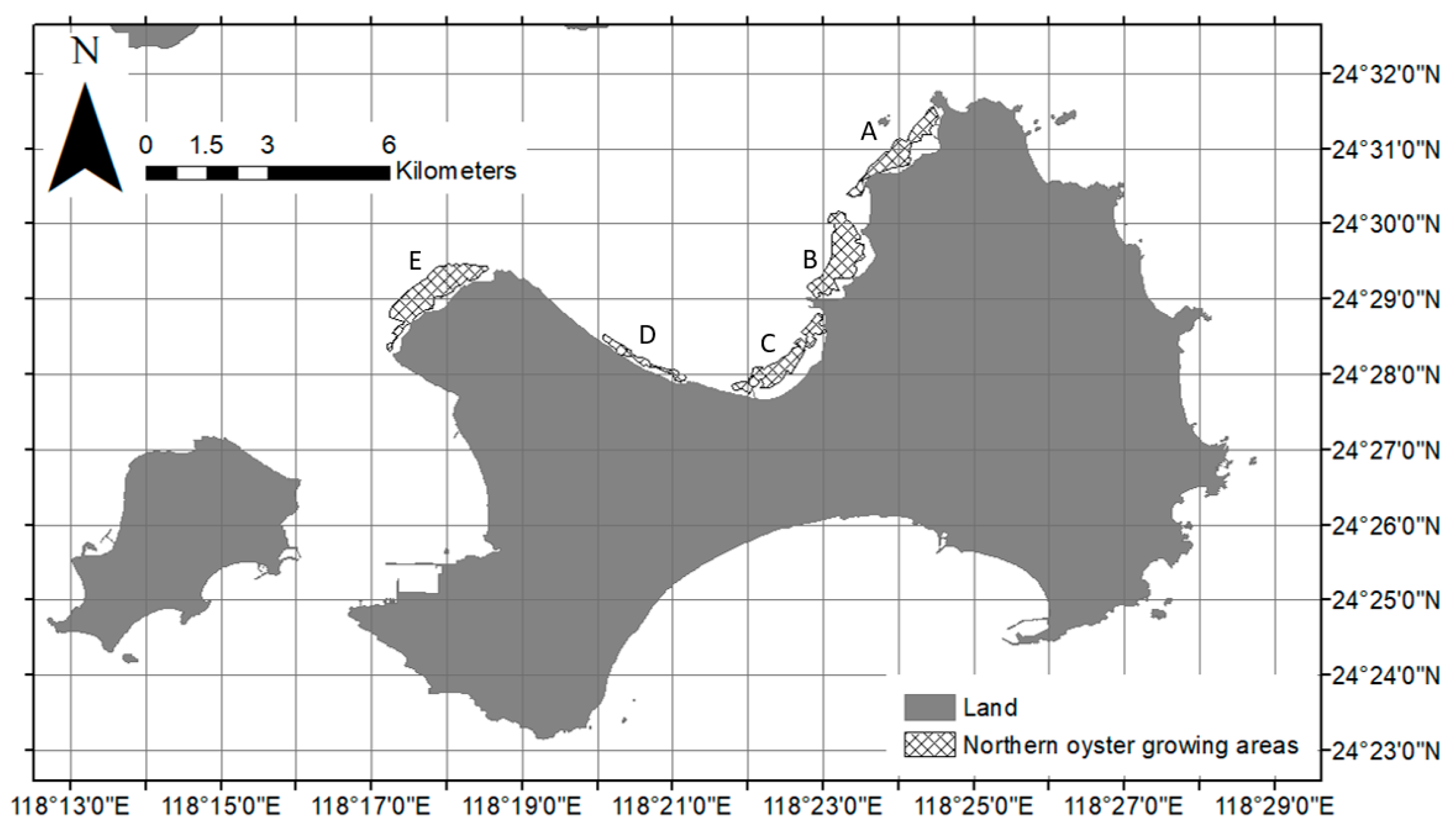
Oyster growth is an important fishing activity in Kinmen. Most oyster-growing areas are located in shallow water in the bay in northern Kinmen, and the five most important are delineated in
Figure 2 (coded A-E in the figure). The annual productivity of oysters is approximately 22 million NTD (about 733 thousand USD), about 30% of all fishery productivity in Kinmen [
19].
Due to the rapid economic growth of China in recent years, the coastal regions of China have seen widespread urbanization, while the island of Kinmen still retains its natural appearance. One of such main development activities is the construction of Xiang’an Airport on newly reclaimed land. In addition to water quality issues, dredging for land reclamation is also considered detrimental to coast stability [
9].
Figure 3 shows the progress of the land reclamation project from 2010 to 2020. A total of 25.58 km
2 of land was reclaimed in the process.
3. Data Availability
Data used by the current study are obtained from several sources. Water quality data near the island of Kinmen is downloaded for the time frame 2005–2021 from the iOcean website [
21]. The time frame covers all stages of the land reclamation project (2010–2018) and provides sufficient baseline information before and after the project. There are three sampling sites near the coast of Kinmen (
Figure 4), and in this study, the one in the semi-enclosed bay with coordinates of (24.467°N, 118.352°E) is chosen. The current study focuses only on this area as it is the area most likely to be affected by the land reclamation project.
Level-2 Landsat 5/7 reflectance data are downloaded from EarthExplorer [
22]. Instead of the newer Landsat 8/9 data, Landsat 5/7 data is used because Landsat 5/7 covers the whole timeframe of 2005–2021, while Landsat 8 did not start working until 2013. Since Landsat 8 and Landsat 5/7 have different band designations, the current study adopts only data from Landsat 5/7. Collection 2 Level-2 data are used because they have been corrected for atmospheric gases, aerosols, water vapor, and surface characteristics before being released [
23] and thus are ready to be used.
Regarding the actual schedule of the land reclamation project, there is no official channel to download or request this information from the Chinese government. The only piece of information available is the on-site billboard [
24]. The total reclaimed area of 25.58
is divided into the phases described in
Table 1.
4. Methodology and Data Analysis
4.1. Derivation of Predictive Statistical Models
Landsat images are used to determine the surface water quality of the entire bay with high spatial and temporal resolutions. Multiple regression-based statistical models are derived to calculate the surface concentration of water constituents from combinations of band reflectance. Following the recommendations of Tu et al. [
25], environmental factors in
Table 2 are included to increase accuracy by accounting for the influence of the gap between water sampling and image dates, energy transfer between water and air, wind speed, and solar radiation.
Table 2 shows all initial predictor (independent) variables in the forward-selection variable selection process.
The relationship between band reflectance and water quality is valid only when the bottom reflection is negligible [
25]. Bottom reflection should not be a concern because the Secchi disk depth (
0.6 m based on the mean Total Suspended Solid (TSS) concentration) [
26] is lower than the mean water depth at the sampling site (
1 m) [
27]. To ensure sufficient depth of water, only images with a water level higher than the mean value (~3 m) during satellite flyovers are chosen [
28]. All Landsat images taken ±7 days from the water sampling dates with water level >3 m are divided into a calibration group and a validation group provided by
Table 3 and
Table 4, respectively.
The forward-selection stepwise regression method is used in building the statistical model based on multiple regression. Minimal Akaike Information Criterion (AIC) is considered when choosing variables. At each step of the selection of variables, only the variable that decreases the most AIC enters the model. A model with minimal AIC explains the most variation with the least number of predictive variables. AIC is a commonly used criterion and is often superior to other selection methods [
29]. The Variation Inflation Factor (VIF) of each selected variable is monitored to keep multicollinearity in check.
The concentrations of two water constituents (TSS and dissolved inorganic nitrogen (DIN)) are the focus. The parameters of the predictive statistical models for TSS and DIN are provided in
Table 5 and
Table 6, respectively. Note that the dependent variables are transformed. The calibration accuracy (represented by the R
2 value) is 0.84 and 0.97 for TSS and DIN, respectively. The validation accuracy is 0.90 and 0.58 for TSS and DIN, respectively. Most accuracy values are considered “Very Good” (defined as R
2 > 0.80 for sediment or R
2 > 0.70 for nitrogen) according to Moriasi et al. [
30]. The only exception is the satisfactory performance (defined as 0.3 < R
2 ≤ 0.60) of the DIN validation accuracy. Scatter plots of measured and predicted TSS and DIN concentrations are provided in
Figure 5 and
Figure 6, respectively.
The variables chosen in the final models show the importance of environmental factors in the determination of water quality constituents using remotely sensed data. Inclusion of temporal differences in both models is deemed to increase accuracy. To predict the TSS concentration, mean air temperature is another important environmental factor, which might be related to water column convection caused by energy transfer between air and water. It was found to alter the convective mass flux up to three orders of magnitude [
31]. Algae and phytoplankton, which are regulated by solar radiation, are closely related to nitrogen concentration, and this interaction is shown in
Table 6.
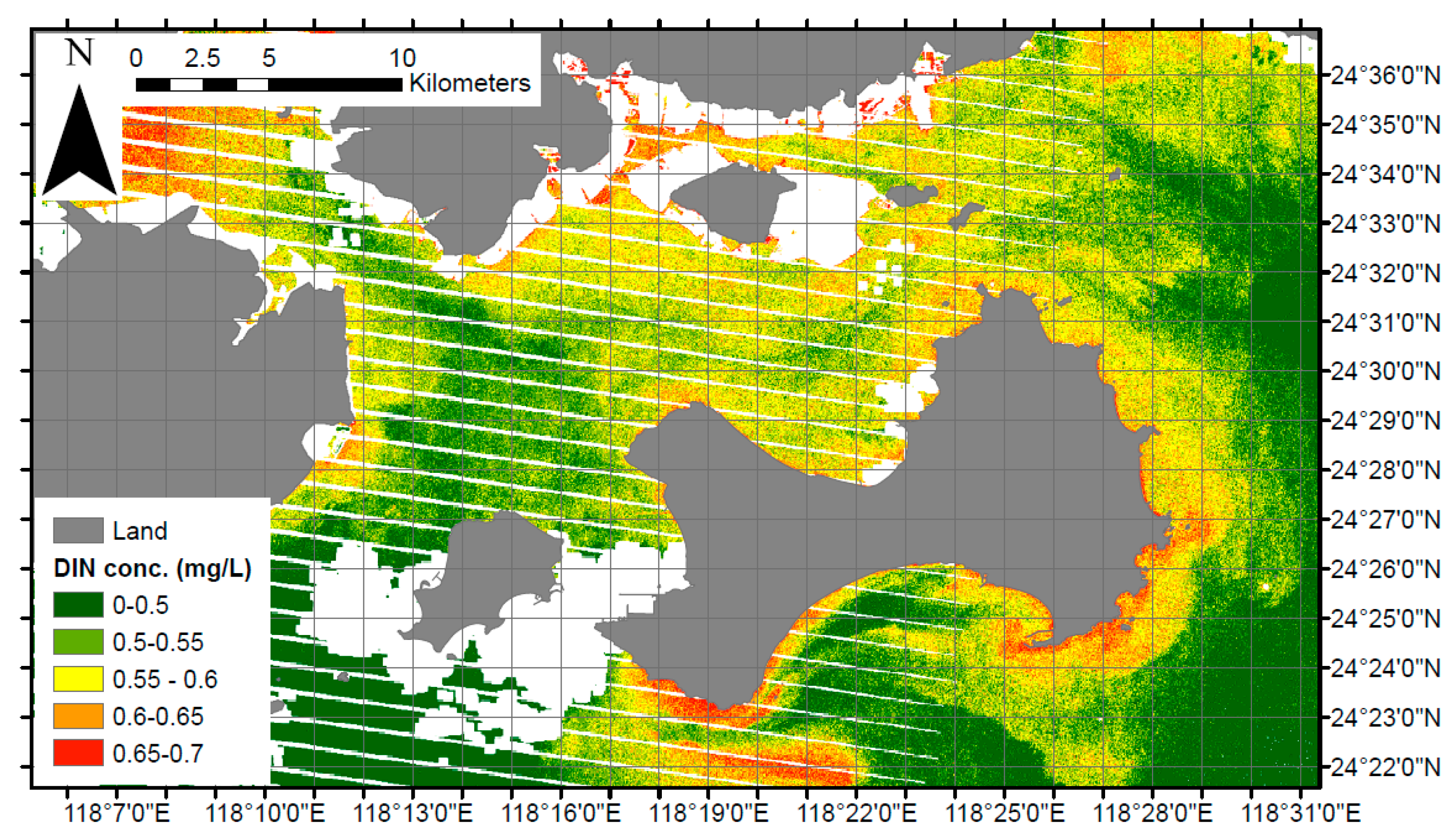
Utilizing the derived statistical models,
Figure 7 and
Figure 8 provide examples of TSS and DIN concentration distributions, respectively, based on Landsat-7 imagery of 8/10/2018. In
Figure 7 and
Figure 8, white-out masks indicate the effect of the failed Landsat-7 scan line corrector (SLC), reclaimed land, cloud cover, or cloud shadow [
32]. Pollutant plumes can be distinguished around the island in
Figure 7 and
Figure 8, with one TSS plume particularly distinguishable in the north of the island (at approximately 24°30′N, 118°21′E). It was possibly caused by dredging activities, but the sediment appears to redeposit quickly so it did not affect water quality at the shore. Because no DIN plume is found in the same area, it can be concluded that the bottom material does not contain a lot of nutrients.
Figure 7 and
Figure 8 also show great variation at different parts of the island’s shore, which is a good demonstration of why remote sensing techniques were chosen by many studies similar to the present one.
4.2. Temporal Variation of Water Quality
To delineate the variation of the concentration of water quality constituents, Landsat images are selected for each season (that is, January–March, April–June, July–September, and October–December) from 2005 to 2021. The water level of all selected images at the flyover is higher than the mean water level of 3 m. A total of 54 images are chosen.
The distribution of the concentration of surface water quality constituents can be calculated for the 54 images utilizing the statistical models in
Table 5 and
Table 6. The mean and maximum concentrations of TSS and DIN in the five oyster-growing areas from 2005 to 2021 are provided in
Figure 9 and
Figure 10, respectively. Note that only an area with a mean depth > 1 m is included in the calculation of the mean and maximum concentration.
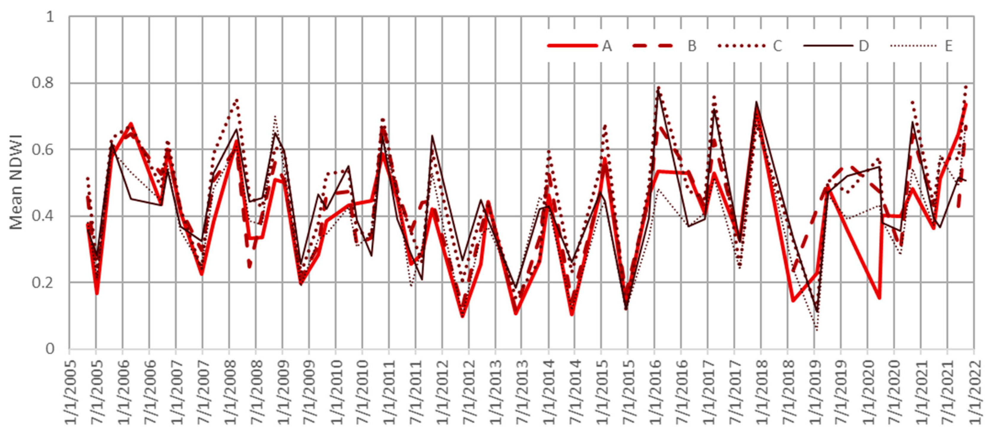
4.3. Temporal Variation of the Coastline Recession
The normalized difference water index (NDWI, given by Equation (1)) is used as a surrogate for the conditions of the coast. In Equation (1),
is the reflectance at the visible green band, and
is the reflectance at the near-infrared band.
NDWI, which detects the existence of water and is insensitive to TSS concentration [
33,
34,
35], has been widely used in coastline determination [
36,
37]. Decreasing NDWI indicates sedimentation of the beach, while increasing NDWI implies shore erosion. The five oyster-growing areas are used again as ‘monitoring areas’. To improve the detection sensitivity, only areas with a mean depth of water <1 m are used, as shown in
Figure 11 below. The seasonal mean NDWI (based on the 54 images) in the five monitoring areas is provided in
Figure 12.
4.4. Factors Impacting Water Quality Constituents and Coast Conditions
An important goal of the current study is to determine the relationship between the land reclamation project and variations in the concentration of water quality constituents and the conditions of the coast. To achieve this goal, another set of statistical models utilizing multiple regression is derived following the process below. Stepwise regression with forward selection with TSS concentration, DIN concentration, or NDWI as the dependent variable is used. The variables listed in
Table 7 are the initial selection of predictor (independent) variables. Disturbed areas (active or cumulative) are directly related to the progress of land reclamation. Tide is known to be the main mechanism to influence sediment diffusion [
6]. The antecedent dry days and 7-day cumulative rainfall depth are related to the amount of sediment washed off by runoff. To explore potentially significant interactions between independent variables, all possible two-way interactions are initially included, but only the main effects are shown in
Table 7 for brevity and clarity of the table. Using forward selection with minimal AIC as a criterion, the statistical models that represent the relationship are provided in
Table 8,
Table 9 and
Table 10. Note that the dependent variables are transformed in the models.
5. Discussion
5.1. Overall Trends of TSS Concentration, DIN Concentration, and Coast Conditions
According to
Figure 9, the concentration of TSS in the bay in northern Kinmen is acceptable for oyster growth (significantly below the hazardous level of 188 mg/L for oysters [
19]) in the observation period of 2005–2021. No long-term increasing or decreasing trend was found for either the mean or maximum value. The mean TSS value reaches 50.58 mg/L in area E on 2/28/2011, and the maximum TSS value is at 96.11 mg/L on the same day.
The TSS concentration shows great short-term variations for all five oyster-growing areas. Using area E as an example, which has the highest maximum TSS concentration of 23.82 mg/L with a standard deviation of 18.89 mg/L. Using available data and assuming a normal distribution for the maximum TSS concentration, the possibility that the maximum TSS concentration reaches 188 mg/L or greater at area E is less than 1 %. Therefore, the oyster-growing industry in the bay in northern Kinmen is unlikely to be jeopardized even with the presence of the nearby land reclamation project.
Similarly, DIN also exhibits a steady trend for long-term concentration with significant short-term variations. Taking into account the rapid development in all coastal cities in China,
Figure 10 implies that the semi-enclosed bay in northern Kinmen is hydrodynamically isolated from the major cities to a certain degree [
5,
38], and the land reclamation activity probably did not significantly alter the circulation of nutrients in the bay.
The trend for coast conditions (using NDWI as a surrogate,
Figure 12) is somehow different. No general trend exists, but two time periods exhibit noticeable trends in NDWI, namely 2008–2013 (sedimentation) and 2018–2021 (erosion). The second period is particularly significant, which might be causally related to the completion of the final phase (July 2016 – December 2018) of the land reclamation project. Longer observations and comprehensive simulations are required to confirm such a trend.
5.2. Factors Influencing TSS Concentration, DIN, and Coast Conditions
The statistical models derived in
Table 8,
Table 9 and
Table 10 revealed factors that influence TSS concentration, DIN concentration, and coast conditions, respectively. Moderate R
2 values limit their use in directly predicting TSS, DIN, or NDWI, but the statistical significance of the individual predictor variable can still be confirmed. For TSS, the interaction between the 7-day cumulative rainfall depth and tide direction (
) is the most significant variable among all five areas. The coefficient for that term suggests that the sediment source is outside the bay (potentially from rainfall-induced runoff from land reclamation sites) as
is positively correlated to TSS (note that the dependent variable in the model is
) during rising tides (i.e., flowing into the bay).
Area C is the only area with TSS that is potentially influenced by the cumulative area () or active area () of the land reclamation project. This is intriguing because area C is located deep in the bay. This finding implies the potential existence of hydrodynamic connections between the interior of a bay and offshore pollution sources. This is a topic worth further study.
For DIN, the interaction between the active area and the 7-day cumulative rainfall depth (
) is significant for all areas. Nevertheless,
and
are mostly not significant. This indicates a “crossover” interaction in which only the two main effects together have explanatory power, and the effect of either main effect alone would be offset by the effect of the interaction [
39]. The result shows an instantaneous connection between the active area and nutrient concentration; however, more active reclamation area and more rainfall appear to decrease the concentration of DIN (note that the dependent variable in the model is
). One reasonable explanation is that runoff from newly reclaimed land dilutes the concentration of nutrients in water. The land reclamation project is confirmed not to have a detrimental influence on nutrient concentration in the bay. Such a conclusion should be accepted with caution as the validation accuracy for DIN estimation is not satisfactory (
Figure 6b).
The coast condition in the monitoring areas A–D is simply affected by the interaction between tide and the 7-day cumulative rainfall depth (
), showing the short-term influence of storms and tides on beach conditions. During rising tides, more antecedent rainfall induces shore erosion (while sedimentation occurs in falling tides). Area E appears to be influenced by different mechanisms, however. The cumulative reclaimed area (
) and interactions involving
are significant factors for the coast condition in monitoring area E. This coincides with what Lin et al. [
40] found: coastline progression in northern Kinmen is a complex process: beach erosion and sedimentation can follow one another at the same location in the short term.
5.3. Implications for the Integrated Coastal Management of Semi-Enclosed Coastlines
The mechanism of interaction between land reclamation and the water quality of a semi-enclosed bay can be complicated. In the case of Xiang’an Airport, land reclamation does not have a direct causal relationship with water quality and coast conditions, whereas studies in other parts of the world had mixed findings.
For suspended sediment, a study in Palu Bay in Indonesia [
41] had a result similar to that of the current study, that the TSS concentration is mostly stable after land reclamation. However, this is not the case for bays with more restricted external access [
42]. The relative alteration of the sea current by land reclamation could be the key factor controlling the outcome of the TSS concentration. A future study that provides empirical criteria on whether the concentration of TSS will be impacted after land reclamation based on the reclaimed area and the geometry of the bay can advance integrated coastal management.
For nutrients, two independent studies conducted by Lyu et al. [
7] and Zhang et al. [
43] both determined that land reclamation contributes significantly to the change of nutrient concentration and can intensify the effect of land-based pollutant inputs. Therefore, the current study could be a special case as the semi-enclosed bay lacks significant land-based pollutant sources. The synergy between land reclamation and land-based pollution is crucial to effective integrated coastal management.
The current study only observes a noted trend in coastline changes after the land reclamation project was completed in 2018. Another study in the Pearl River Delta in China [
44] with a much longer (about 40 years) observation time frame confirmed that land reclamation causes long-term geomorphological changes. Therefore, the geomorphological effect of Xiang-an Airport is worth close monitoring before it can contribute to our understanding of integrated coastal management.
The current study also highlights the importance of transboundary corporation in environmental issues. Due to the lack of key information (such as the actual land reclamation schedule) released by the Chinese government, the current study can only use the best information available on the Internet. An integrated management scheme can only be achieved with the cooperation of all parties.
6. Conclusions
Utilizing remotely sensed data, this study investigates the two main concerns of Kinmen residents caused by a nearby land reclamation project, namely the deterioration of water quality and the change in coastline. TSS and DIN are used to represent the general trends of the water quality constituents and NDWI for the coast conditions.
The TSS concentration, DIN concentration, and coast conditions do not show a clear trend for the observation time frame of 2005–2021. From 2005 to 2021, the TSS concentration is generally low in the bay regardless of the existence of the major land reclamation project. Statistical analyses gauge the possibility for TSS to achieve a hazardous level (188 mg/L) in the bay at less than 1 %. The DIN concentration shows an even more steady trend despite the rapid urbanization on the Chinese coast. Regarding coast conditions (surrogated by NDWI), there is a significant rising trend (i.e., coast erosion) after the completion of the project in 2018 despite the long-term stability, but such a recent trend can only be confirmed with longer observations in the future.
Factors that influence short-term variations in TSS concentration and coast conditions are also analyzed by models derived from multiple regression, and neither the actively reclaimed area () nor cumulative reclaimed area () is among the main influencers. The 7-day cumulative rainfall depth () positively and significantly influences TSS only when the tide ( increases, suggesting that the sediment source is outside the bay (potentially from rainfall-induced runoff from the land reclamation sites). Coast conditions are influenced by similar factors, with larger storms followed by shore erosion at rising tides (while shore sedimentation at falling tides).
DIN concentration is affected by , but a larger actively reclaimed area decreases DIN concentration, not increasing it, suggesting a dilution effect from rainfall-induced runoff. Newly claimed land is not a source of nutrients in this case. Such a conclusion should be accepted with caution as the validation accuracy for DIN estimation is not satisfactory.
In summary, the concentration of TSS, the concentration of nutrient (DIN), and the conditions of the coast are in satisfactory numerical range and stable. All three indicators (TSS, DIN, and NDWI) are not negatively affected by the land reclamation project after utilizing multiple regression models. However, some intriguing findings are found from the current study and require further investigation in the future:
(1) The concentration of TSS in area C deep in the bay is potentially affected by the cumulative area () or active area () of the land reclamation project. It might imply the potential existence of hydrodynamic connections between the interior of a bay and offshore pollution sources; and
(2) The coast condition in area E is affected not only by the cumulative reclaimed area () but also by several interactions involving . More delicate investigations are needed to understand the erosion/sedimentation mechanisms in that area.
Author Contributions
Conceptualization, Y.-c.H.; Methodology, M.-c.T.; Software, M.-c.T. and Y.-c.H.; Validation, M.-c.T.; Formal analysis, M.-c.T.; Investigation, M.-c.T. and Y.-c.H.; Resources, M.-c.T.; Data curation, M.-c.T. and Y.-c.H.; Writing—original draft, M.-c.T.; Writing—review & editing, M.-c.T.; Visualization, M.-c.T.; Supervision, M.-c.T.; Project administration, M.-c.T.; Funding acquisition, M.-c.T. All authors have read and agreed to the published version of the manuscript.
Funding
This research received no external funding.
Data Availability Statement
All data available from publicly accessible sources delineated in the article.
Conflicts of Interest
The authors declare no conflict of interest.
References
- Freeman, L.A.; Corbett, D.R.; Fitzgerald, A.M.; Lemley, D.A.; Quigg, A.; Steppe, C.N. Impacts of Urbanization and Development on Estuarine Ecosystems and Water Quality. Estuaries Coasts 2019, 42, 1821–1838. [Google Scholar] [CrossRef]
- Abal, E.G.; Dennison, W.C.; Greenfield, P.F. Managing the Brisbane River and Moreton Bay: An integrated research/management program to reduce impacts on an Australian estuary. Water Sci. Technol. 2001, 43, 57–70. [Google Scholar] [CrossRef] [PubMed]
- Alber, M. A conceptual model of estuarine freshwater inflow management. Estuaries 2002, 25, 1246–1261. [Google Scholar] [CrossRef]
- van Maren, D.S.; Oost, A.P.; Wang, Z.B.; Vos, P.C. The effect of land reclamations and sediment extraction on the suspended sediment concentration in the Ems Estuary. Mar. Geol. 2016, 376, 147–157. [Google Scholar] [CrossRef]
- Mao, X.; Hong, G. Analysis of dredging impact of an airport reclamation on hydrodynamic environment in a semi-enclosed bay with force tide. In Proceedings of the Thirteenth Pacific-Asia Offshore Mechanics Symposium, Jeju, Republic of Korea, 14–17 October 2018. [Google Scholar]
- Yan, H.-K.; Wang, N.; Yu, T.-L.; Fu, Q.; Liang, C. Comparing effects of land reclamation techniques on water pollution and fishery loss for a large-scale offshore airport island in Jinzhou Bay, Bohai Sea, China. Mar. Pollut. Bull. 2013, 71, 29–40. [Google Scholar] [CrossRef]
- Lyu, H.; Song, D.; Zhang, S.; Wu, W.; Bao, X. Compound effect of land reclamation and land-based pollutant input on water quality in Qinzhou Bay, China. Sci. Total Environ. 2022, 826, 154183. [Google Scholar] [CrossRef]
- Zhu, H.; Bing, H.; Yi, H.; Wu, Y.; Sun, Z. Spatial Distribution and Contamination Assessment of Heavy Metals in Surface Sediments of the Caofeidian Adjacent Sea after the Land Reclamation, Bohai Bay. J. Chem. 2018, 2018, 2049353. [Google Scholar] [CrossRef] [Green Version]
- Demir, H.; Otay, E.N.; Work, P.A.; Borekci, O.S. Impacts of Dredging on Shoreline Change. J. Waterw. Port Coast. Ocean Eng. 2004, 130, 170–178. [Google Scholar] [CrossRef]
- Mostafa, Y.E.S. Environmental impacts of dredging and land reclamation at Abu Qir Bay, Egypt. Ain Shams Eng. J. 2012, 3, 1–15. [Google Scholar] [CrossRef] [Green Version]
- Wang, W.; Liu, H.; Li, Y.; Su, J. Development and management of land reclamation in China. Ocean Coast. Manag. 2014, 102, 415–425. [Google Scholar] [CrossRef]
- Duan, H.; Zhang, H.; Huang, Q.; Zhang, Y.; Hu, M.; Niu, Y.; Zhu, J. Characterization and environmental impact analysis of sea land reclamation activities in China. Ocean Coast. Manag. 2016, 130, 128–137. [Google Scholar] [CrossRef]
- CNA News. Mainland China Pumping Sea Sand to Build Airport Threatens to Erode Kinmen Coast. 2013. Available online: https://www.cna.com.tw/Proj_County/012/cht_news/201307310482.aspx?page=74 (accessed on 12 October 2022).
- Kinmen News. The Construction of Xiamen Xiang’an Airport Has a Profound Impact on Kinmen. 2017. Available online: https://www.kinmen.gov.tw/News_Content2.aspx?n=98E3CA7358C89100&sms=BF7D6D478B935644&s=99239E94F08960A3&Create=1 (accessed on 12 October 2022).
- Gholizadeh, M.H.; Melesse, A.M.; Reddi, L. A Comprehensive Review on Water Quality Parameters Estimation Using Remote Sensing Techniques. Sensors 2016, 16, 1298. [Google Scholar] [CrossRef] [PubMed] [Green Version]
- Kinmen County Government. 2022 Kinmen Big Data Analytics. Available online: https://www.kinmen.gov.tw/bigdata/cp.aspx?n=4A61630A0002B0D4 (accessed on 4 October 2022).
- Kinmen News. The Orientation of Kinmen’s Development and the Conception of Industry Forward-looking Planning. 2013. Available online: https://www.kmdn.gov.tw/1117/1271/1276/224453/?cprint=pt (accessed on 5 October 2022).
- Kinmen County Government. Advance Planning for Additional Passenger Terminals on Daidian and Eidian Islands. 2016. Available online: https://ws.kinmen.gov.tw/Download.ashx?u=LzAwMS9VcGxvYWQvMzA0L3JlbGZpbGUvMC8zMTg1Mi80MTRjNmY3Ni04MmE4LTRjNjgtOTA2Zi1iMzA4NDAyNjk5MmEucGRm&n=RmNoMi3ln7rmnKzos4fmlpnokpDpm4bliIbmnpAucGRm (accessed on 31 October 2022).
- Huang, W.-B. The Impact of Silt Deposition along the Coast of Kinmen on the Oyster Aquaculture Production Area—A Preliminary Analysis. 2014. Available online: https://ws.kinmen.gov.tw/Download.ashx?u=LzAwMS9VcGxvYWQvMzIzL3JlbGZpbGUvMC8xODc4OS8xMDPlubTluqbph5HploDmsr%2Fmtbfmt6Tms6XmsonnqY3lsI3niaHooKPppIrmrpbnlJ%2FnlKLljYDkuYvlvbHpn7%2FliJ3mraXoqZXmnpDmnJ%2FmnKvloLHlkYoucGRm&n=MTAz5bm05bqm6YeR6ZaA5rK%2F5rW35rek5rOl5rKJ56mN5bCN54mh6KCj6aSK5q6W55Sf55Si5Y2A5LmL5b2x6Z%2B%2F5Yid5q2l6KmV5p6Q5pyf5pyr5aCx5ZGKLnBkZg%3D%3D (accessed on 4 October 2022).
- Google Earth. 24.50°N, 118.35°E, Elevation 24.4 km. 2022. Available online: http://www.google.com/earth/index.html (accessed on 12 October 2022).
- Taiwan Ocean Conservation Administration. iOcean Ocean Conservation Network. 2022. Available online: https://iocean.oca.gov.tw/OCA_OceanConservation/PUBLIC/Marine_WaterQuality_v2.aspx (accessed on 18 September 2022).
- USGS. EarthExplorer. 2022. Available online: https://earthexplorer.usgs.gov/ (accessed on 24 September 2022).
- USGS. Landsat Collection 2 Level-2 Science Products. 2022. Available online: https://www.usgs.gov/landsat-missions/landsat-collection-2-level-2-science-products (accessed on 19 September 2022).
- Anyuan Co. Ltd. Aerial Observation of the Land Reclamation Project for Xiangan Airport. 2016. Available online: https://read01.com/zh-tw/6jBR8k.html#.Yy1Y53ZBxPY (accessed on 23 September 2022).
- Tu, M.-C.; Smith, P.; Filippi, A.M. Hybrid forward-selection method-based water-quality estimation via combining Landsat TM, ETM+, and OLI/TIRS images and ancillary environmental data. PLoS ONE 2018, 13, e0201255. [Google Scholar] [CrossRef] [PubMed] [Green Version]
- Gurlin, D. Near Infrared-red Models for the Remote Estimation of Chlorophyll-α Concentration in Optically Complex Turbid Productive Waters: From in Situ Measurements to Aerial Imagery. Doctoral Dissertation, University of Nebraska, Lincoln, NE, USA, 2012. [Google Scholar]
- Ocean Data Bank. Water Depth Database. 2022. Available online: https://www.odb.ntu.edu.tw/bathy/ (accessed on 18 September 2022).
- Dayu Tide Table. Dayu Tide Table. 2022. Available online: http://chaoxibiao.net (accessed on 18 September 2022).
- Hastie, T.; Tibshirani, R.; Friedman, J. The Elements of Statistical Learning: Data Mining, Inference and Prediction; Springer: New York, NY, USA, 2001. [Google Scholar]
- Moriasi, D.; Gitau, M.W.; Pai, N.; Daggupati, P. Hydrologic and water quality models: Performance measures and evaluation criteria. Trans. ASABE 2015, 58, 1763–1785. [Google Scholar]
- Kirillin, G.; Engelhardt, C.; Golosov, S. Transient convection in upper lake sediments produced by internal seiching. Geophys. Res. Lett. 2009, 36, L18601. [Google Scholar] [CrossRef]
- Sayler, K. Landsat 4-7 Collection 2 (C2) Level 2 Science Product (L2SP) Guide; EROS: Sioux Falls, SD, USA, 2021. [Google Scholar]
- Hou, X.; Feng, L.; Duan, H.; Chen, X.; Sun, D.; Shi, K. Fifteen-year monitoring of the turbidity dynamics in large lakes and reservoirs in the middle and lower basin of the Yangtze River, China. Remote Sens. Environ. 2017, 190, 107–121. [Google Scholar] [CrossRef]
- Ehmann, K.; Kelleher, C.; Condon, L.E. Monitoring turbidity from above: Deploying small unoccupied aerial vehicles to image in-stream turbidity. Hydrol. Process. 2018, 33, 1013–1021. [Google Scholar] [CrossRef]
- Garg, V.; Aggarwal, S.P.; Chauhan, P. Changes in turbidity along Ganga River using Sentinel-2 satellite data during lockdown associated with COVID-19. Geomat. Nat. Hazards Risk 2020, 11, 1175–1195. [Google Scholar] [CrossRef]
- Ozelkan, E. Water Body Detection Analysis Using NDWI Indices Derived from Landsat-8 OLI. Pol. J. Environ. Stud 2020, 29, 1759–1769. [Google Scholar] [CrossRef]
- Alcaras, E.; Falchi, U.; Parente, C.; Vallario, A. Accuracy evaluation for coastline extraction from Pléiades imagery based on NDWI and IHS pan-sharpening application. Appl. Geomat. 2022, 1–11. [Google Scholar] [CrossRef]
- Wang, J.; Hong, H.; Zhou, L.; Hu, J.; Jiang, Y. Numerical modeling of hydrodynamic changes due to coastal reclamation projects in Xiamen Bay, China. Chin. J. Oceanol. Limnol. 2012, 31, 334–344. [Google Scholar] [CrossRef]
- Loftus, G.R. On interpretation of interactions. Mem. Cogn. 2015, 6, 312–319. [Google Scholar] [CrossRef] [Green Version]
- Lin, J.-Q.; Ren, J.-H.; Shen, M.-Y. Survey of Coastal Landscape Resources in Kinmen National Park and Conservation Management Planning. 2016. Available online: https://www.kmnp.gov.tw/resource/conservication/127.pdf (accessed on 4 October 2022).
- Koropitan, A.F.; Purba, M.; Pranowo, W.S.; Rusydi, M. Numerical model of ocean currents, sediment transport, and geomorphology due to reclamation planning in Palu Bay. Adv. Environ. Sci. 2019, 11, 87–96. [Google Scholar]
- Gao, G.D.; Wang, X.H.; Bao, X.W.; Song, D.; Lin, X.P.; Qiao, L.L. The impacts of land reclamation on suspended-sediment dynamics in Jiaozhou Bay, Qingdao, China. Estuar. Coast. Shelf Sci. 2018, 206, 61–75. [Google Scholar] [CrossRef]
- Zhang, P.; Su, Y.; Liang, S.-K.; Li, K.-Q.; Li, Y.-B.; Wang, X.-L. Assessment of long-term water quality variation affected by high-intensity land-based inputs and land reclamation in JiaozhouBay, China. Ecol. Indic. 2017, 75, 210–219. [Google Scholar] [CrossRef] [Green Version]
- Zhang, W.; Xu, Y.; Hoitink, A.J.F.; Sassi, M.G.; Zheng, J.; Chen, X.; Zhang, C. Morphological change in the Pearl River Delta, China. Mar. Geol. 2015, 363, 202–219. [Google Scholar] [CrossRef]
| Disclaimer/Publisher’s Note: The statements, opinions and data contained in all publications are solely those of the individual author(s) and contributor(s) and not of MDPI and/or the editor(s). MDPI and/or the editor(s) disclaim responsibility for any injury to people or property resulting from any ideas, methods, instructions or products referred to in the content. |
© 2023 by the authors. Licensee MDPI, Basel, Switzerland. This article is an open access article distributed under the terms and conditions of the Creative Commons Attribution (CC BY) license (https://creativecommons.org/licenses/by/4.0/).


