1. Introduction
The geoid is the gravitational equipotential surface that coincides with the global tideless mean sea surface and extends into the interior of the continents [
1]. In the spherical approximation, Stokes’s formula combines global gravity anomaly data with kernel functions to integrate for geoid modeling [
2]. It is a challenge to obtain global gravity data, and gravity data within a certain radius of the calculation point are used to participate in the calculation, resulting in missing gravity signals outside the radius and causing truncation errors. Molodensky et al. proposed a modification of Stokes’s formula by combining terrestrial gravity data with the global geopotential model (GGM) [
3], where the terrestrial gravity data and GGM provide the short-wavelength and long-wavelength components, respectively, to reduce the truncation error.
Several deterministic and stochastic modifications to Stokes’s formula are proposed. The deterministic approaches consider the truncation error, and the terrestrial gravity data and the global geopotential model error are ignored. The main deterministic modification methods have Molodenskii [
3], Wong and Gore [
4], Meissl [
5], Heck and Grüninger [
6], Vaníček and Kleusberg [
7], Vaníček and Sjöberg [
8], and Featherstone [
9]. Sjöberg proposed biased, unbiased, and optimum stochastic modifications to Stokes’s formula [
10,
11,
12]. The stochastic modifications simultaneously consider the error in truncation, the terrestrial gravity data, and the global geopotential model. The least squares (LS) are applied to calculate the modification parameters to minimize the expected global mean square error (MSE).
Sjöberg proposed the least squares modification of Stokes’s formula with additive corrections (LSMSA) [
13], which used the terrestrial gravity anomaly as the integration term and adopted the stochastic least squares modification methods with the additive corrections to calculate the geoid height. Featherstone gave a combination of deterministic and stochastic modifications [
14], using stochastic modifications when the error variance is reliable, and, vice versa, the deterministic modifications are recommended. Ellmann compared two deterministic and three stochastic modification methods for Stokes’s formula [
15], and the results showed no significant differences between the deterministic and stochastic modifications. Stokes’s formula’s deterministic and stochastic modifications have been widely used in geoid modeling [
16,
17,
18,
19,
20,
21].
As the solution of the geodetic second boundary value problem, Hotine’s formula is also applied to geoid modeling [
22]. Hotine’s formula uses the integration term of gravity disturbances calculated from the ellipsoidal heights. The modification of Hotine’s formula is similar to Stokes’s Jekeli-derived Molodensky-type truncation coefficients of Hotine’s formula [
23]. Vaníček et al. [
24], Rapp [
25], Alberts and Klees [
26], and Changyou Zhang proposed the deterministic modifications to the Hotine’s formula [
27]. Novák [
28], Sjöberg, and Eshagh et al. used airborne gravity data for geoid modeling based on Hotine’s formula [
29], and Featherstone summarized the deterministic, stochastic, and hybrid modifications to Hotine’s formula and their practical applications [
30].
Märdla proposed the least squares modification of Hotine’s formula with additive corrections (LSMHA) and used part of Northern Sweden in Europe as the study area for geoid modeling [
31]; the results showed that there were no significant differences between the LSMHA and LSMSA. Işık et al. applied the LSMHA and LSMSA methods to calculate the Colorado geoid based on airborne and terrestrial gravity data [
32]. Sakil et al. adopted the LSMHA method for geoid modeling using gridded and non-gridded gravity data [
33]. Abbak et al. provided a scientific software package for the LSMHA method [
34].
Based on the above studies, this paper applies two deterministic and three stochastic modifications to Stokes’s and Hotine’s formulas. The terrestrial gravity data are used as the integration term to refine the quasigeoid of Jilin Province. In the modeling, we reasonably analyze the selection of modification parameters according to the global RMSE values. The study region is divided into plain and mountainous areas, following the topographic differences, in order to explore the influence of topography on the modeling of different integration formulas and all types of modifications.
2. Motivation and The Study Objective
This study aimed to contribute with the numerical assessment of five different modification methods for Stokes’s and Hotine’s formulas by computing a number of quasigeoid models of the Jilin Province, China. High-precision regional quasigeoid plays a vital role in practical engineering applications, earth science research, etc. In past studies, deterministic and stochastic modifications have been widely used for geoid refinement. Meanwhile, the development of Global Navigation Satellite System (GNSS) also provides the possibility for the application of Hotine integration. In order to make the experiments richer, we conducted the comparison between different integration formulas and different modification methods at the same time and chose the same modification parameters as much as possible to make the comparison results more reliable. The means of the expected global RMSE and evaluation by the GPS/leveling points make the selection of the best modification method. Through this experiment, we expect to establish a high-precision quasigeoid model for Jilin Province and provide some reference for geoid modeling by different modification methods.
3. Data and Methods
3.1. Study Area and Data
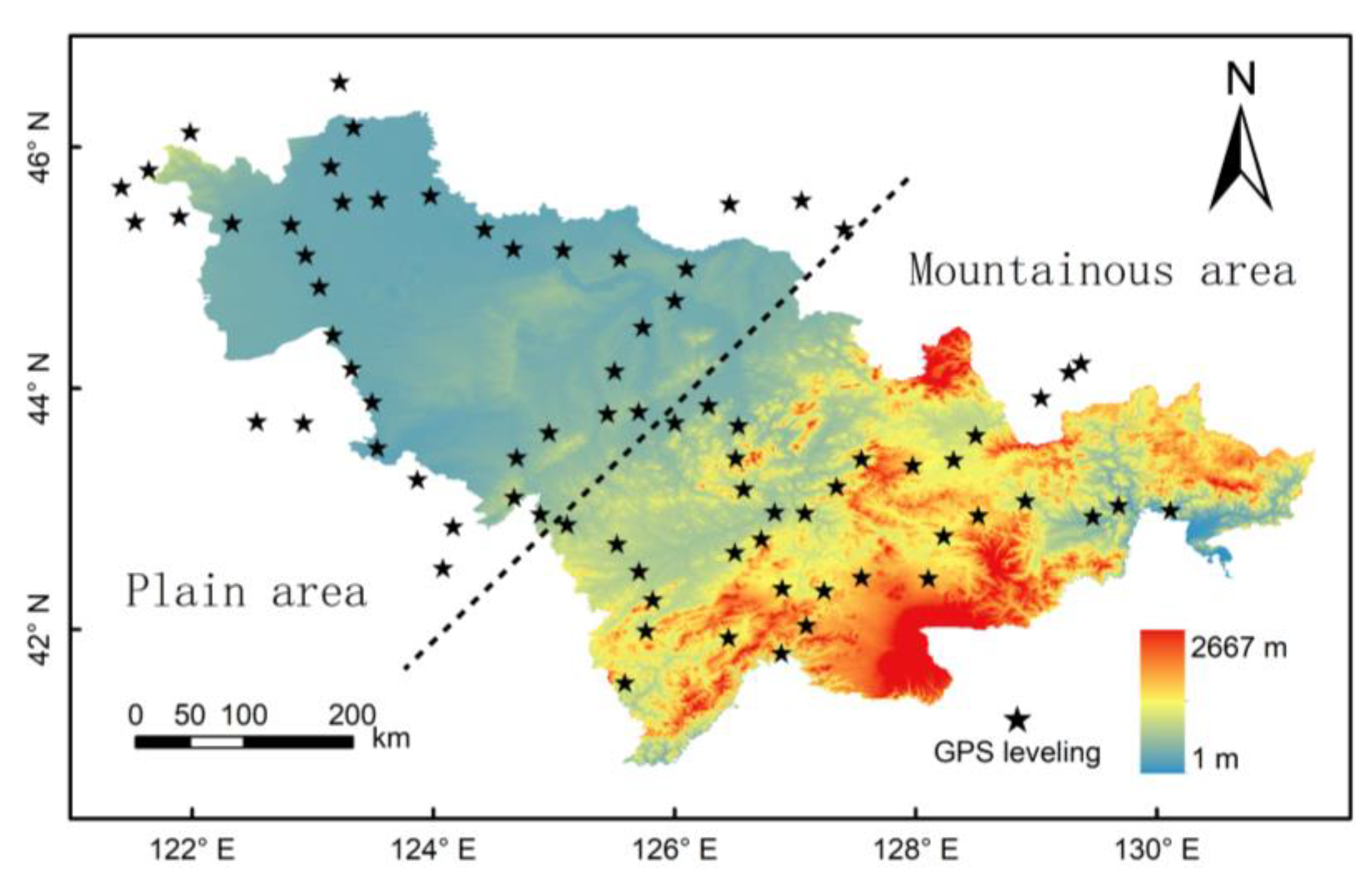
Jilin Province (40.9°–46.3°N, 121.6°–131.3°E) is located in the central part of Northeast China (
Figure 1), with a total area of about 187,400
. The topography of Jilin Province gradually rises from west to east, with a maximum elevation of about 2667 m and an average elevation of about 405 m, showing a significant difference in height between the east and west. The study area was divided into plain and mountainous regions based on the topographic discrepancies. The average elevation of the plain and mountainous areas is about 170 m and 600 m, respectively.
The choice of GGM plays an essential role in geoid refinement. The XGM2019 model was released in 2019 with the degree and order fully expanded to 2159 and a resolution of about 5 min, performing globally more consistently than many other models [
35]. The model consists of three main data sources: the GOCO06s model composed of satellite gravity data, the 15-minute ground gravity anomaly dataset provided by the US National Geospatial-Intelligence Agency (NGA), and the 1-minute augmentation dataset derived from topography.
The terrestrial gravity data cover the 0.5° range outside the study area, which is referenced to the China Geodetic Coordinate System 2000 (CGCS2000) datum. The terrestrial gravity measurements are dense in the western parts, whereas the data are sparsely distributed in the eastern parts of the study area. The free-air gravity anomalies of the discrete gravity points are not smooth enough for direct interpolation. We used complete Bouguer, topographic, and isostatic correction and performed a gridding process to obtain a 2.5′ × 2.5′ free-air gravity anomaly grid. The gravity-disturbance grid was generated from gravity anomaly, using an existing geoid model (XGM2019 gravity field model up to 2190 degree/order) according to Equation (1), which has no ellipsoidal height information.
The SRTM3 digital elevation model (DEM) was used in the calculation of the influence of topography on the geoid. In the Chinese region, the SRTM3 data elevation accuracy is overall higher than 1:250,000 DEM [
36]. The 77 high-precision GPS/leveling points were used to evaluate the geoid modeling in and around Jilin Province, including 41 in plain and 36 in mountainous areas. The GPS/leveling points use the CGCS2000 national geodetic coordinate system and the 1985 national height datum of China as horizontal and vertical datum, respectively, with ±1.0 cm accuracy in horizontal and vertical.
3.2. Geoid Modeling
The geoid height is calculated from the Stokes’s formula as follows [
37]:
where
R represents the mean Earth radius;
is the normal gravity on the reference ellipsoid
is the geocentric angle;
is the gravity anomaly;
is the surface element of the unit sphere
; and
is the Stokes’s function expressed as a series of the Legendre polynomial,
, over the sphere [
37]:
The geoid heights calculated from Hotine’s formula is performed analogously to Stokes’s formula as follows [
22]:
and
where
is the gravity disturbance, and
is the Hotine’s function.
The calculation of the geoid using Equations (2) and (4) requires global coverage of gravity data, which are difficult to obtain. Therefore, the integration range is limited with a small domain,
, surrounding the computation point. Moreover, considering the influence of external topography and other factors on the geoid, the modeling equation is shown as follows [
13]:
where
is the approximate geoid undulation,
is the combined topographic effect,
is the combined downward continuation effect,
is the combined atmospheric effect, and
is the combined ellipsoidal effect.
3.2.1. Approximate Geoid Undulation
The approximate geoid undulation based on Stokes’s formula is as follows [
12]:
and
The first term of Equation (7) corresponds to the near zone component of the geoid, and the other term indicates the far zone component.
is the modified Stokes’s function,
is the terrestrial gravity anomaly, L is the upper limit of the harmonics to be modified in Stokes’ function,
M is the upper limit of the truncation degree of the gravity field model,
is the modification parameter,
is the modification parameter of the GGM gravity anomaly, and
is the Laplace harmonics of the gravity anomaly that is calculated as follows [
38]:
where
is the equatorial radius of the reference ellipsoid,
is the geocentric radius,
is the GGM coefficient, and
is the fully normalized surface spherical harmonics.
The approximate geoid undulation of Hotine’s formula is calculated as follows [
31]:
where
is the modified Hotine’s function,
is the terrestrial gravity disturbance, and
is the Laplace harmonics of the gravity disturbance.
3.2.2. Deterministic Modifications
The deterministic modification gives modification parameters to reduce truncation errors. The WG modification is the removal of the lower degree part of the original kernel function and renders modeling formulas less sensitive to low-frequency errors in the terrestrial gravity signal by partially filtering them out [
30]. The WG modification of Stokes’s and Hotine’s formulas is calculated as follows [
4,
24]:
The VK modification combines the WG and Molodensky modifications, intending to minimize the upper bound of the truncation error in the least squares sense [
15]. We take
T = L in this paper, and the formulas are given as follows [
7,
27]:
where
represents the modification coefficients determined from the solution of a set of linear equations.
Modification parameter
is calculated as follows [
15]:
where
and
are the modified and unmodified Molodensky-type truncation coefficient, respectively. The coefficients
and
are calculated by the formulas given by Jekeli and Paul [
23,
39].
The WG and VK modification parameter
values are shown in
Table 1 [
15]:
3.2.3. Stochastic Modifications
The stochastic least squares modifications (biased, unbiased, and optimum) determine the modification parameters
and
by taking the minimum value according to the global MSE. The global MSE is differentiated with respect to each
(
n = 0, 1, 2, ..., L) and equated to zero as follows [
40]:
where
is the element of the design matrix, and
is the element of the observable vector. Their calculations differ in different modification types, as detailed in Märdla [
41].
The linear system of Equation (19) can be written in matrix form as follows:
The modification parameter
was approximately estimated by the least squares. In the biased modification, it can be calculated directly. For the unbiased and optimum modification, parameter
is calculated by using Singular Value Decomposition (SVD) to solve the ill-conditioned problem of linear equations [
42].
The
values of three stochastic least squares modifications are shown in
Table 2. There is no calculation difference of
in the Stokes’s and Hotine’s formulas.
3.2.4. Additive Corrections
In the geoid modeling using the Stokes’s and Hotine’s formulas, it is assumed that the topography and atmospheric masses do not exist above the geoid, and the shape of the Earth is approximated as a sphere. Based on these assumptions, additive corrections need to be incorporated. Here, additive corrections of Hotine’s formula are introduced.
The combined topographic effect includes direct and indirect effects of topography and is calculated as follows [
42]:
where
is the mean topographic mass density, and
H is the elevation of the topography.
The combined downward continuation effect is computed by using the following [
31,
41]:
where
and
where
is the spherical radius of the computation point, and
is the vertical gradient of gravity disturbance and calculated as follows [
43]:
where
is the spatial distance between the computation point and the running point.
The combined atmospheric effect is computed by using the following [
44]:
where
is the atmospheric mass density at sea level.
The combined ellipsoidal effect can be adopted [
34]:
where
is the zero term of Molodensky-type truncation coefficients.
3.3. Error Propagation
The approximate geoid undulation is calculated by combining terrestrial gravity data with GGM in geoid modeling. However, the GGM coefficients and the terrestrial gravity data contain noise, which propagates into the computed geoid undulations. Considering the noise, Equation (7) can be expressed in spectral form as follows [
15]:
and
where
and
denote the spectral errors of the terrestrial and GGM-derived gravity anomalies, respectively.
According to the spectral form of the true geoid undulation,
, the global MSE of the Stokes’s formula for geoid modeling is as follows [
12]:
and
where
. The right side of the equation in order represents the error contribution due to GGM, truncation, and terrestrial gravity data; and
represents the terrestrial gravity anomaly error degree variances, which were calculated with reference to Ellmann [
39].
The global MSE of Hotine’s formula is similar to Stokes’s formula and is given as follows [
31]:
4. Results
4.1. Parameters of Geoid Modeling
The accuracy of the geoid modeling is affected by the modification limits, integral radius and terrestrial gravity data error variance. The choice of the modification limit M is directly related to the quality of the long wavelength component of the GGM calculation in the geoid, and the modification limit L minimizes the value of the modified formula outside the integration radius. Both high and low limits have been applied in the geoid modeling for modification limits M and L. The integral radius and the terrestrial gravity data error variance impact the geoid’s short wavelength component. This study gave an integration radius of 0.5 degrees.
4.1.1. Modification Limits
We chose the appropriate modification limits
M and
L based on the global RMSE. In the stochastic least squares modifications, the modification limit
M is taken to be equal to
L by default. Taking the terrestrial gravity data error variance as 1
and the modification limits
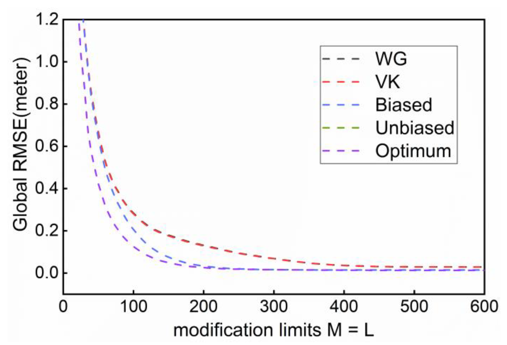
M = L, the global RMSE variation of Stokes’s formula for different modification limits
M and
L are shown in
Figure 2.
There was no significant discrepancy between the Stokes’s and Hotine’s formulas, reaching a maximum of about 1 cm when the modification limits were small and decreasing to 1 mm as the limits increased.
In the global RMSE variation, the WG provided a similar error to the VK modification, and the unbiased and optimum modifications remain consistent. With increasing modification limits, the global RMSE of all modifications showed a decreasing tendency, and stochastic modifications declined significantly faster than deterministic modifications when the modification limits were less than 200. The global RMSE tended to change steadily as the limits increased to 400, and WG and optimum modifications generated the maxi-mum and minimum error values, respectively. The final values are shown in
Table 3. The global RMSE of stochastic modifications was about 1.3 cm, which is significantly lower than the deterministic modifications of approximately 2.9 cm.
In geoid modeling, the integral range is restricted to a specific radius, causing a shortage of gravity signals. This influence can be reduced by using a larger modification limit M. However, an excessive limit, M, may introduce extra GGM potential coefficient errors. Combined with the global RMSE variation in
Figure 2, we took the stochastic modification limit
M = L = 450 in the subsequent geoid modeling.
When the modification limits were taken as
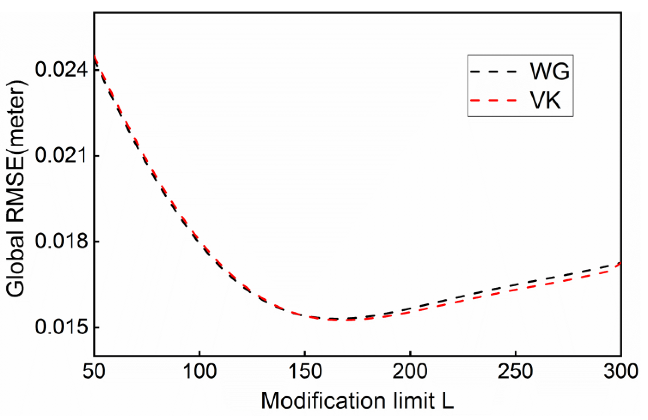
M = L, the global RMSE of the deterministic modifications had a larger global RMSE and lower geoid modeling accuracy than the stochastic modification. To improve the modeling accuracy and facilitate a comparison with stochastic modifications, limit M of the deterministic modifications was set the same as that of the stochastic modifications. The global RMSE variation of Stokes’s formula for deterministic modifications with different modification limits (
L) is shown in
Figure 3.
The global RMSE variation of Hotine’s formula was similar to that of Stokes’s. There was no stable trend for the error of the deterministic modification as the limit L increased. The global RMSE decreases up to 160 to reach the minimum value and then increases slowly. Therefore, the limits M = 450 and L = 160 of deterministic modifications for subsequent analysis and geoid modeling.
4.1.2. Integral Radius
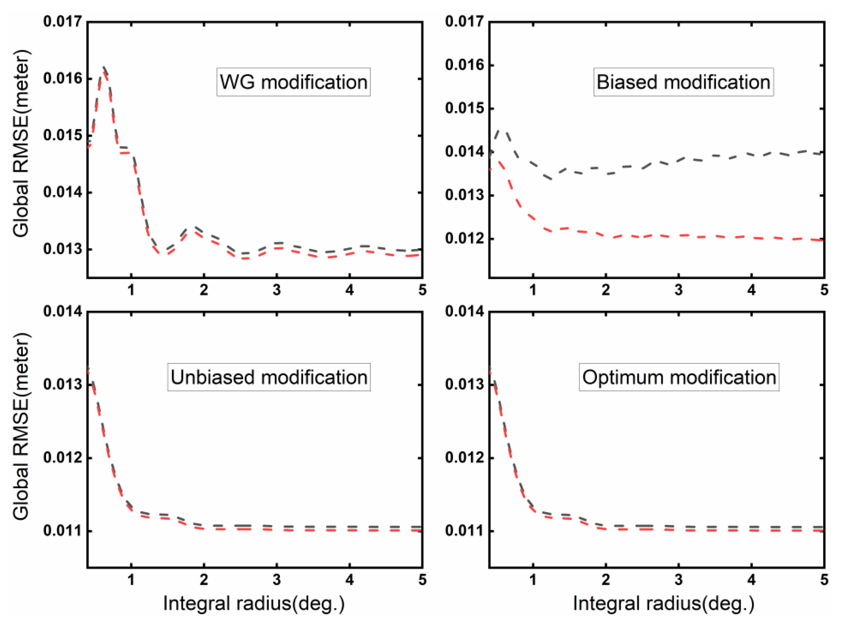
For different modification methods, there are other trends of global RMSE variation with the integral radius. Choosing a suitable integral radius can maximize the use of terrestrial gravity data and ensure the accuracy of geoid modeling simultaneously. We took the terrestrial gravity data error variance as 1
to research the effect of the integral radius on the global RMSE. The variation of the global RMSE with the integral radius is shown in
Figure 4.
The global RMSE of VK modification produced a similar variation to the WG modification, and we only show the WG modification instead. Both deterministic and biased modifications oscillated at a small integration radius. With the increase of integration radius, more terrestrial gravity data are involved in the geoid calculation, and the global RMSE of each modification decreases and stabilizes.
Among all the modifications, the global RMSE of Hotine’s formula was smaller than that of Stokes’s formula, which was more evident in the biased modifications, where the difference reached about 2 mm, and less than 1 mm in the remaining modifications. The main reason for this discrepancy is the calculation of the truncation error term. Substituting the of biased modification, the truncation error becomes . At degrees less than M, there is a relatively significant difference of between Stokes’s and Hotine’s formula, which increases with integral radius, leading to a more considerable of global RMSE in the biased modification. For the other modifications, the value and the small GGM error degree variances, , caused no significant difference between Stokes’s and Hotine’s formulas.
The integral radius was taken as 0.5°, and the difference between the global RMSE and steady value was less than 3 mm. From a theoretical point of view, it could be desirable to consider the integral radius to be as large as possible. We defined the integral radius as 0.5°, combining global RMSE and terrestrial gravity data utilization.
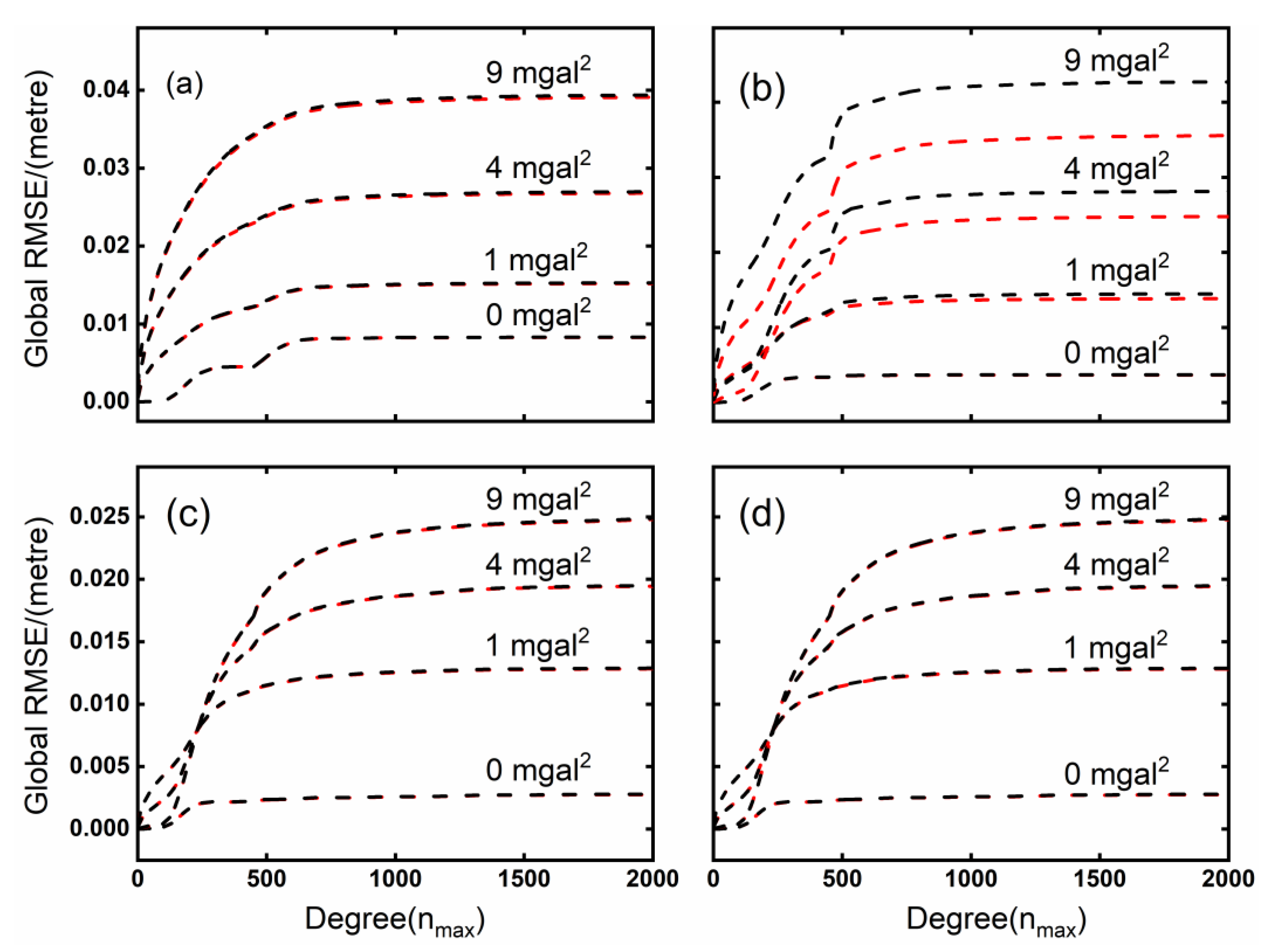
4.1.3. Terrestrial Gravity Data Error Variance
The terrestrial gravity data error degree variance needs to be determined in the stochastic least squares modifications modeling and the calculation of the global RMSE. The accuracy of the measured terrestrial gravity data is not uniform in the study area, and terrestrial gravity data error variance is replaced by a constant. We took the terrestrial gravity data error variance as 0, 1, 4, and 9
, respectively, to study its effect on the global RMSE. The result is shown in
Figure 5.
The results in
Figure 5 showed that the global RMSE increased accordingly as the terrestrial gravity data error variance increased. The global RMSE contained only the truncation error and the GGM potential coefficient error when the terrestrial gravity data error variance was taken as 0
, and the stochastic modifications’ values were significantly smaller than the deterministic modifications’ values. Compared to the deterministic modifications, stochastic modifications have a small value of truncation and GGM potential coefficient error.
The global RMSE of unbiased and optimum modification was smaller than the biased and deterministic modification, and this tendency is more pronounced as terrestrial gravity data error variance increases. Compared to other type modifications, the modified truncation coefficient, , of the biased ones has a larger difference between Stokes’s and Hotine’s formula, which increases with the rise of terrestrial gravity data error variance, causing a relatively large discrepancy in the global RMSE. In the subsequent geoid modeling, we took the terrestrial gravity data error variance as 1 .
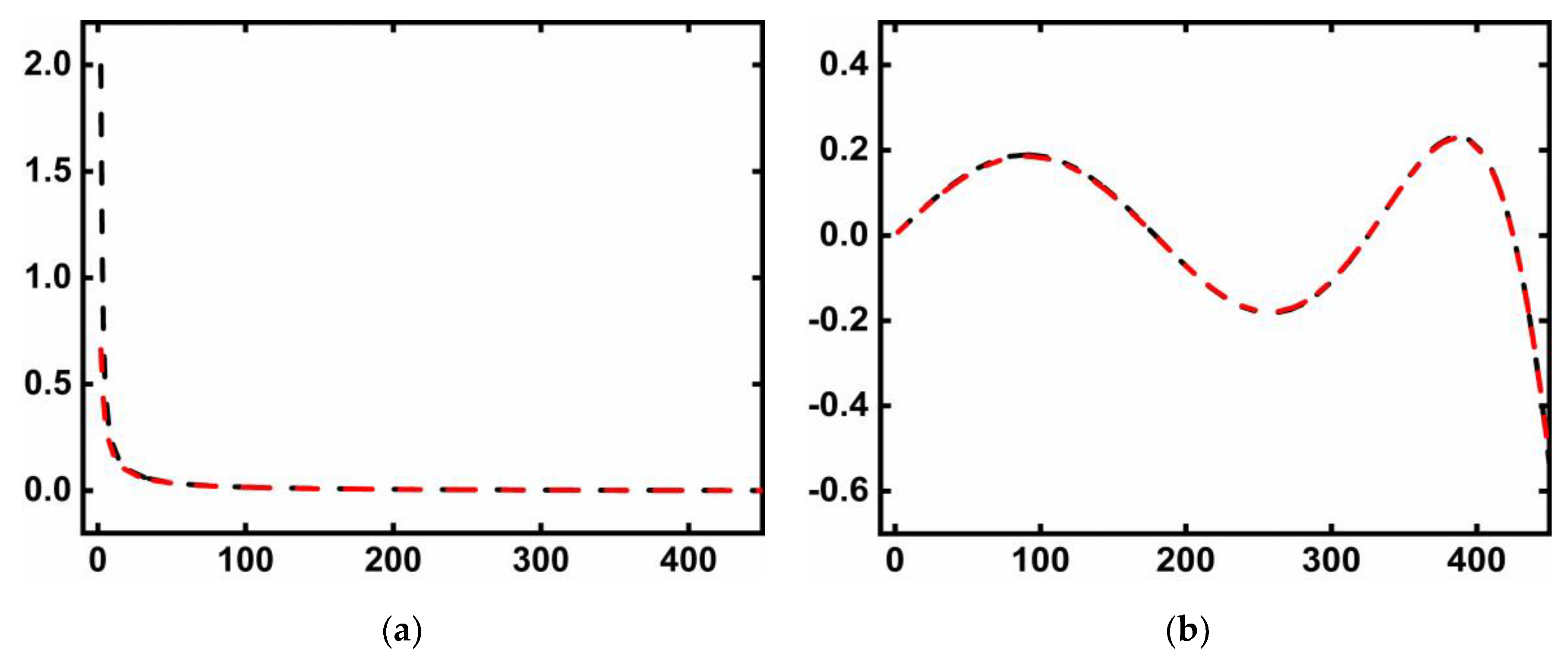
4.1.4. Modification Parameters
The modification parameters
are essential for calculating the approximate geoid undulation, affecting the kernel function value and the degree of GGM contribution, respectively. Variations of the parameters are shown in
Figure 6.
The WG and VK modifications produced a similar variation to the biased modification for the parameter . The biased modification parameter decreased rapidly and stabilized, and the initial value of Hotine’s formula was smaller than that of Stokes’s formula. Unlike the biased modification, unbiased and optimum modification parameters’ did not stabilize at zero value; instead, they oscillated around it.
For the parameter , under the joint action of the parameter and the truncation coefficient, , etc., all five modification methods had similar variations to the parameter of the biased modification. The initial value of Hotine’s was smaller than Stokes’s formula.
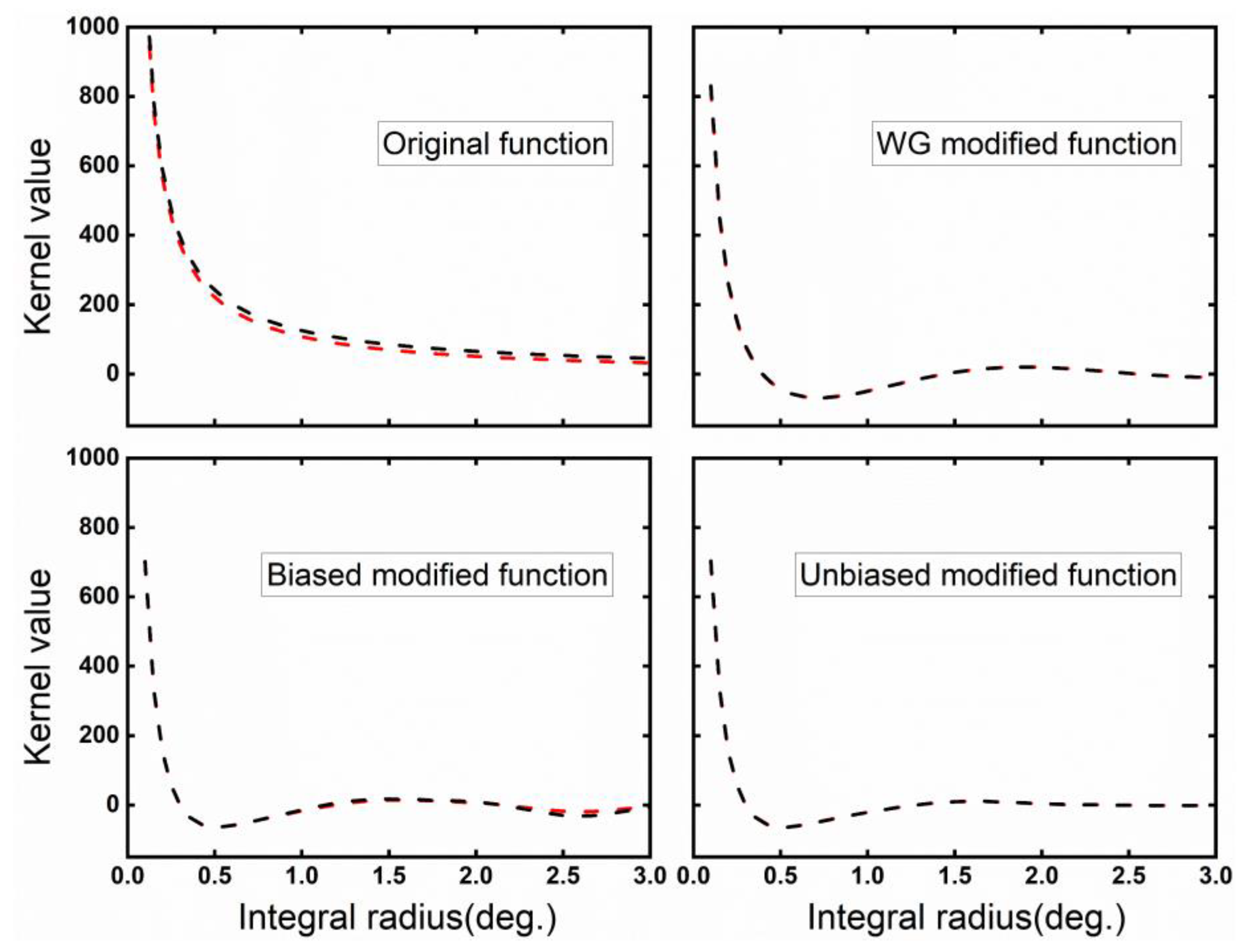
The difference between the modified and original kernel functions is shown in
Figure 7. The modified kernel function decreased faster than the original kernel function and approached the zero value more rapidly, which converged gradually after reaching a minimum value. The stochastic modified kernel function changed faster than the deterministic one. The difference between Stokes’s and Hotine’s kernel functions reached 20 in the original and biased modifications and was less than 1 in the remaining modifications.
4.1.5. Expected Global RMSE
The expected global RMSE is used to compare different geoid modeling methods, and their values are shown in
Table 4, where
,
, and
represent the error contribution due to the GGM, truncation, and terrestrial gravity data, respectively.
The global RMSE of Hotine’s formula was slightly smaller than that of Stokes’s formula, and the differences between them were more evident in the biased modification. The differences of and between Stokes’s and Hotine’s formula in the biased one are larger than in other modifications, resulting in higher discrepancies in the GGM and truncation error. The truncation error and terrestrial gravity data error were effectively reduced in the stochastic modifications, which had a smaller global RMSE than the deterministic modification. The global RMSE of WG and VK modifications was equal and unbiased, and optimum was better than that of the biased.
4.2. Accuracy Evaluation
4.2.1. Accuracy of XGM2019
We calculated the geoid heights of the XGM2019 model and obtained the maximum and minimum values of 26.26 m and 4.12 m, respectively. There is a smooth variation in the western plains area and a relatively drastic one in the eastern mountainous area.
We evaluated the accuracy of the XGM2019 model in the study area, using GPS-leveling points; the results are shown in
Table 5. The XGM2019 model had an error range value of 24.65 cm and an accuracy of 5.40 cm in Jilin Province. In the plain area, the accuracy is higher at 4.29 cm, and the error range is 21.97 cm. The accuracy is relatively poor in mountainous areas, at 6.43 cm.
The differences in gravity signal between the terrestrial gravity data and the XGM2019 model are shown in
Table 6. The maximum and minimum values of terrestrial gravity signals were less than eight times and four times that of the STD. The terrestrial gravity signal contains high-frequency information, and the STD is greater than the model gravity signal.
4.2.2. Accuracy Comparison of Quasigeoid in Jilin Province
Based on the XGM2019 model, we used the deterministic and stochastic modified Stokes’s and Hotine’s formulas to refine the quasigeoid of Jilin Province. After adding the additive corrections, the results showed that the refined gravimetric geoid height had a reduced range and was smoother overall than the approximate geoid undulation.
Among the additive corrections, the values of the combined topographic effect and downward continuation effect were larger, reaching the decimeter level. In comparison, there was a smaller value of the combined atmospheric and ellipsoidal effects, at about the millimeter level. The additive corrections displayed consistency with the topographic elevation, with a more significant number of corrections in the steep topography area and a lower correction in the gentle topography area.
The study area used a normal height system with a quasigeoid datum. We adopted GPS/leveling points as the control, performing least-squares combined with seven parameters fitting of the gravimetric geoid to obtain a fitted quasigeoid model adapted to the area [
45]. The 44 GPS/leveling points were evenly selected to participate in the fitting, and the remaining 33 points were evaluated, including 18 in the plain and 15 in mountainous areas.
where
and
where
e is the first eccentricity of the reference ellipsoid, and
and
represent the geodetic latitude and longitude of GPS/leveling station. The results of the accuracy comparison in Jilin Province are shown in
Table 7.
The refined quasigeoid had a significant improvement in accuracy and error range compared with the XGM2019 model, the maximum accuracy was improved by 2.5 cm, and the error range was reduced by about 50%, making the stochastic modifications were more noticeable.
Each refined quasigeoid model achieved the same level of accuracy. The maximum difference in accuracy between Stokes’s and Hotine’s formulas was less than 0.1 cm. Moreover, in the same integral formula, there was a maximum difference of 0.2 cm among the modification methods. These differences were less than the GPS/leveling points accuracy and did not provide substantial differences among the quasigeoid models.
Although the accuracy of the deterministic and stochastic modifications was essentially the same throughout the study area, the error range of deterministic modifications was significantly larger than that of the stochastic modifications. The STD reflects the error outlier, and the phenomenon indicates that the error values of deterministic modifications are more concentrated in zero values compared to stochastic modifications. This leads to the possibility that the accuracy of deterministic modifications may be better than stochastic modifications in some areas.
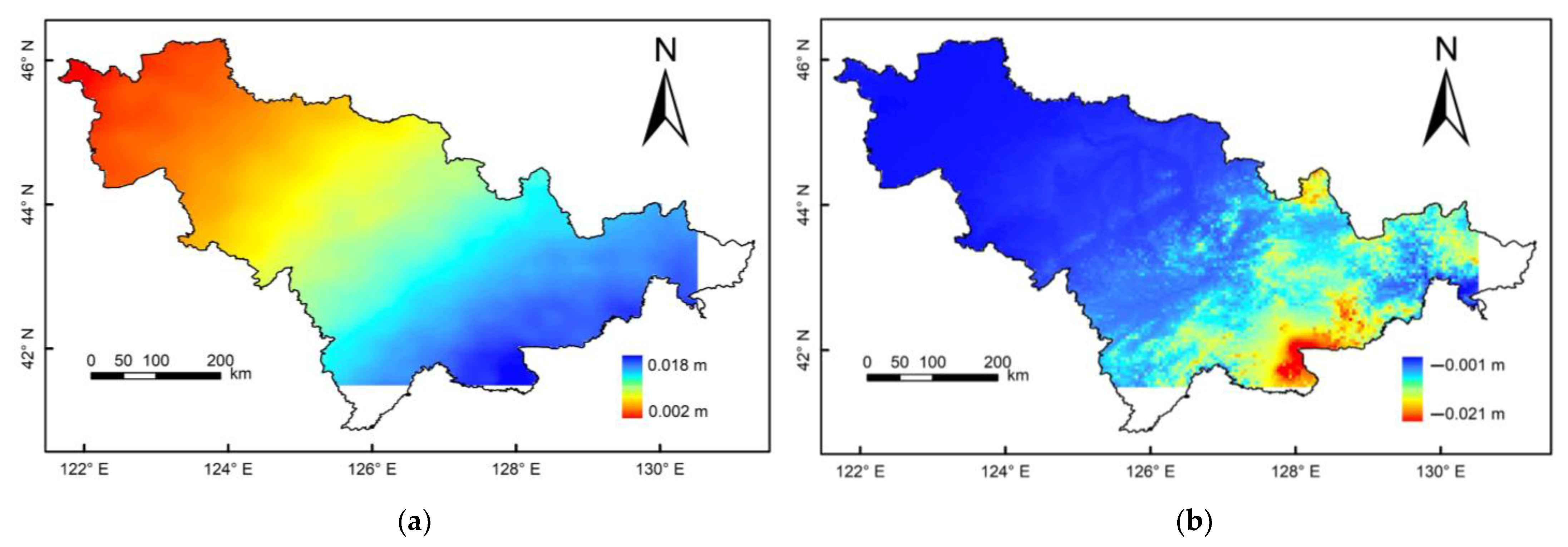
The differences between Stokes’s and Hotine’s formulas for calculating approximate geoid undulation and combined downward continuation effect is shown in
Figure 8, with more minor differences in the remaining additive corrections. The difference increased with the topography, millimeter level in the western plain area, and reached the centimeter level in the eastern mountainous area, which could not be ignored in the geoid refinement. Compared with the combined downward continuation effect, the differences in approximate geoid undulation changed more smoothly.
4.2.3. Accuracy Comparison of Refined Quasigeoid in Different Area
The results of accuracy comparison in plain and mountainous areas are shown in
Table 8 and
Table 9, respectively.
Compared to XGM2019, the deterministic and stochastic modifications improved the accuracy in the plain area by a maximum of 2.3 and 1.9 cm, respectively. Stokes’s and Hotine’s formulas provided the same level of accuracy in the one type of modification, with a maximum difference of 0.1 cm. The deterministic ones were better than stochastic modifications in accuracy and error range, with maximum differences up to 0.5 and 3.4 cm, respectively. The WG and VK modifications had similar accuracy, and there were no substantial differences among the stochastic modifications.
Compared to XGM2019, the deterministic and stochastic modifications improved the accuracy in the mountainous area by a maximum of 2.6 cm and 3.3 cm, respectively. The accuracy in mountainous regions was lower than that in plain areas, although the accuracy values of each modification were more improved in mountainous regions than in plain areas. Stokes’s and Hotine’s formulas provided the same level of accuracy in the one type of modification. The stochastic modifications outperformed the deterministic modifications in mountainous areas and improved accuracy and error range by up to 17% and 28%, respectively, compared to deterministic modifications. The WG and VK modifications had similar accuracy, and there were no substantial differences among the stochastic modifications in mountainous areas.
5. Discussion
Stokes’s and Hotine’s formulas are used to refine the quasigeoid, which can effectively improve the original model’s accuracy. Based on XGM2019, we evaluated the accuracy of Stokes’s and Hotine’s formulas by using five modified kernel functions for the case of Jilin province. Considering that topographic undulation is an influential factor in geoid refinement, we divided the study area into plain and mountainous regions for evaluation.
Across the study area, the accuracy evaluation results were consistent with the ones of Ellmann [
15] and Märdla et al. [
31] and did not provide substantial discrepancies between different integral formulas and modification methods. In contrast, the accuracy of deterministic and stochastic modifications showed relatively significant differences in different topographic areas, plain areas with a 0.5 cm difference, and 0.7 cm difference in high mountain areas. Although the difference was smaller than the GPS/leveling points accuracy, we preferred to make the following choices within the study area: using deterministic modifications in plain areas and stochastic modifications in mountainous areas.
In the parameters’ selection of the deterministic modifications, the same approach as the stochastic modifications was used in this paper, in which the modification parameters were selected according to the global RMSE taken as the minimum. The deterministic modifications only considered the truncation error term in theory. However, we included terrestrial data and model coefficient errors in selecting the modification limits and achieved better accuracy in the refinement of the quasigeoid.
Stochastic modifications to refine the quasigeoid require evaluating the gravity signal and error properties. This paper uses global models for calculating gravity signal or error degree variance, which may not necessarily represent the area of interest. Moreover, the GPS/leveling points used to evaluate the geoid model are distributed as evenly as possible in the study area. Due to external factors such as topography, we could not access evenly distributed GPS/leveling points. In future work, we will work on these aspects to refine the quasigeoid model with higher accuracy.
GNSS provides a convenient approach for obtaining ellipsoidal heights. When refining the geoid, there is no need to convert the ellipsoidal height to physical height. Hotine’s formula can be used to convey an accuracy comparable to that of Stokes’s formula, enriching the theory and practice of geoid refinement.
6. Conclusions
In this study, we used two deterministic modifications and three stochastic least squares modifications of Stokes’s and Hotine’s formulas to calculate the expected global RMSE, approximate geoid undulation, and additive effects to refine the quasigeoid of Jilin province. The refined model was evaluated by GPS/leveling points. Based on the case study in the area of Jilin Province, China, the conclusions can be summarized as follows:
In geoid modeling, the variation of the modification limits and terrestrial gravity data error variance significantly affected the global RMSE, and the integral radius variations had a relatively small influence. Using the same correction parameters, theoretically, Hotine’s formula modeling accuracy was better than Stokes’s formula, and the stochastic modifications outperformed the deterministic ones, wherein unbiased and optimum modifications had the best results.
GPS/leveling points were used to fit and evaluate each refined geoid model. Relative to the original model, the refined quasigeoid accuracy was significantly improved. Stokes’s and Hotine’s formulas provided the same accuracy in Jilin province, China. Meanwhile, different types of modifications all exhibited the same level of accuracy and did not differ significantly.
Although mountainous areas had a greater degree of refinement than plain areas, the accuracy of the plain regions was still significantly better than that of mountainous areas based on the XGM2019 model. Deterministic modifications outperformed stochastic modifications in the plain areas. Suitable modification limits could improve deterministic modification modeling accuracy. In the mountainous areas, where measured terrestrial gravity data were less available, stochastic modifications were preferred to deterministic modifications.
Author Contributions
Conceptualization, Q.W., F.X. and G.Z.; methodology, Q.W., G.Z. and L.Z.; formal analysis, Q.W. and G.Z.; investigation, B.W.; data curation, B.W. and L.Z.; writing—original draft preparation, Q.W. and G.Z.; writing—review and editing, Q.W. and G.Z.; supervision, Q.W. and F.X.; project administration, Q.W. All authors have read and agreed to the published version of the manuscript.
Funding
This research was Funded by Technology Innovation Center for Land Engineering and Human Settlements, Shaanxi Land Engineering Construction Group Co., Ltd., and Xi’an Jiaotong University (2021WHZ0080).
Data Availability Statement
Not applicable.
Conflicts of Interest
The authors declare no conflict of interest.
References
- Wang, C. Research on Sea Area Airborne Gravity Survey Technology and Geoid Rapid Construction Method. Ph.D. Thesis, China University of Geosciences, Beijing, China, 2021. [Google Scholar] [CrossRef]
- Stokes, G.G. On the variation of gravity on the surface of the Earth. Trans. Camb. Phil. Soc. 1849, 8, 672–695. [Google Scholar]
- Molodenskii, M.S. Methods for Study of the External Gravitational Field and Figure of the Earth; Jerusalem, Israel Program for Scientific Translations, 1962; The Office of Technical Services, United States Department of Commerce: Washington, DC, USA, 1962. [Google Scholar]
- Wong, L.; Gore, R. Accuracy of Geoid Heights from Modified Stokes Kernels. Geophys. J. Int. 1969, 18, 81–91. [Google Scholar] [CrossRef] [Green Version]
- Meissl, P. Preparations for the Numerical Evaluation of Second Order Molodensky Type Formulas; Ohio State University Columbus Department of Geodetic Science and Surveying: Columbus, OH, USA, 1971. [Google Scholar]
- Heck, B.; Grüninger, W. Modification of Stokes’ integral formula by combining two classical approaches. In Proceedings of the XIX IUGG General Assembly, Vancouver, BC, Canada, 9–22 August 1988; Volume 2, pp. 319–337. [Google Scholar]
- Vaníček, P. The Canadian geoid-Stokesian approach. Manuscr. Geod. 1987, 12, 86–98. [Google Scholar]
- Vaníček, P.; Sjöberg, L.E. Reformulation of Stokes’s theory for higher than second-degree reference field and modification of integration kernels. J. Geophys. Res. Solid Earth 1991, 96, 6529–6539. [Google Scholar] [CrossRef]
- Featherstone, W.; Evans, J.; Olliver, J. A Meissl-modified Vaníček and Kleusberg kernel to reduce the truncation error in gravimetric geoid computations. J. Geod. 1998, 72, 154–160. [Google Scholar] [CrossRef]
- Sjöberg, L.E. Least-Squares modification of Stokes’ and Vening-Meinez’ formula by accounting for truncation and potential coefficients errors. Manuscr. Geod. 1984, 9, 209–229. [Google Scholar]
- Sjöberg, L.E. Refined least squares modification of Stokes’ formula. Manuscr. Geod. 1991, 16, 367–375. [Google Scholar]
- Sjöberg, L.E. A general model for modifying Stokes’ formula and its least-squares solution. J. Geod. 2003, 77, 459–464. [Google Scholar] [CrossRef]
- Sjöberg, L.E. A computational scheme to model the geoid by the modified Stokes formula without gravity reductions. J. Geod. 2003, 77, 423–432. [Google Scholar] [CrossRef]
- Featherstone, W. Band-limited kernel modifications for regional geoid determination based on dedicated satellite gravity field missions. Gravity Geoid 2002, 341–346. [Google Scholar]
- Ellmann, A. Two deterministic and three stochastic modifications of Stokes’s formula: A case study for the Baltic countries. J. Geod. 2005, 79, 11–23. [Google Scholar] [CrossRef]
- Omang, O.; Forsberg, R. The northern European geoid: A case study on long-wavelength geoid errors. J. Geod. 2002, 76, 369–380. [Google Scholar] [CrossRef]
- Šprlák, M. Generalized geoidal estimators for deterministic modifications of spherical Stokes’ function. Contrib. Geophys. Geod. 2010, 40, 45–64. [Google Scholar] [CrossRef] [Green Version]
- Li, X.; Wang, Y. Comparisons of geoid models over Alaska computed with different Stokes’ kernel modifications. J. Geod. Sci. 2011, 1, 136–142. [Google Scholar] [CrossRef]
- Abbak, R.A.; Sjöberg, L.E.; Ellmann, A.; Ustun, A. A precise gravimetric geoid model in a mountainous area with scarce gravity data: A case study in central Turkey. Stud. Geophys. Geod. 2012, 56, 909–927. [Google Scholar] [CrossRef]
- Sjöberg, L.E.; Gidudu, A.; Ssengendo, R. The Uganda gravimetric geoid model 2014 computed by the KTH method. J. Geod. Sci. 2015, 5, 35–46. [Google Scholar] [CrossRef] [Green Version]
- Ågren, J.; Strykowski, G.; Bilker-Koivula, M.; Omang, O.; Märdla, S.; Forsberg, R.; Ellmann, A.; Oja, T.; Liepins, I.; Parseliunas, E.; et al. The NKG2015 gravimetric geoid model for the Nordic-Baltic region. In Proceedings of the 1st Joint Commission 2 and IGFS Meeting International Symposium on Gravity, Geoid and Height Systems, Thessaloniki, Greece, 19–23 September 2016. [Google Scholar] [CrossRef]
- Hotine, M. Mathematical Geodesy; US Environmental Science Services Administration: Rockville, MD, USA, 1969. [Google Scholar]
- Jekeli, C. Global Accuracy Estimates of Point and Mean Undulation Differences Obtained from Gravity Disturbances, Gravity Anomalies and Potential Coefficients; Technical Report 288; The Ohio State University: Columbus, OH, USA, 1979. [Google Scholar]
- Vanicek, P.; Zhang, C.; Sjoberg, L.E. A comparison of Stokes’s and Hotine’s approaches to geoid computation. Manuscr. Geod. 1992, 17, 29–35. [Google Scholar]
- Rapp, R.H. A comparison of altimeter and gravimetric geoids in the Tonga Trench and Indian Ocean areas. Bull. Géod. 1980, 54, 149–163. [Google Scholar] [CrossRef]
- Alberts, B.; Klees, R. A comparison of methods for the inversion of airborne gravity data. J. Geod. 2004, 78, 55–65. [Google Scholar] [CrossRef]
- Zhang, C. Estimation of dynamic ocean topography in the Gulf Stream area using the Hotine formula and altimetry data. J. Geod. 1998, 72, 499–510. [Google Scholar] [CrossRef]
- Novák, P.; Kern, M.; Schwarz, K.P.; Sideris, M.G.; Heck, B.; Ferguson, S.; Hammada, Y.; Wei, M. On geoid determination from airborne gravity. J. Geod. 2003, 76, 510–522. [Google Scholar] [CrossRef]
- Sjöberg, L.E.; Eshagh, M. A geoid solution for airborne gravity data. Stud. Geophys. Geod. 2009, 53, 359–374. [Google Scholar] [CrossRef]
- Featherstone, W. Deterministic, stochastic, hybrid and band-limited modifications of Hotine’s integral. J. Geod. 2013, 87, 487–500. [Google Scholar] [CrossRef] [Green Version]
- Märdla, S.; Ellmann, A.; Ågren, J.; Sjöberg, L.E. Regional geoid computation by least squares modified Hotine’s formula with additive corrections. J. Geod. 2018, 92, 253–270. [Google Scholar] [CrossRef]
- Işık, M.S.; Erol, B.; Erol, S.; Sakil, F.F. High-resolution geoid modeling using least squares modification of Stokes and Hotine formulas in Colorado. J. Geod. 2021, 95, 1–19. [Google Scholar] [CrossRef]
- Sakil, F.F.; Erol, S.; Ellmann, A.; Erol, B. Geoid modeling by the least squares modification of Hotine’s and Stokes’ formulae using non-gridded gravity data. Comput. Geosci. 2021, 156, 104909. [Google Scholar] [CrossRef]
- Abbak, R.A.; Ellmann, A.; Ustun, A. A practical software package for computing gravimetric geoid by the least squares modification of Hotine’s formula. Earth Sci. Inform. 2022, 15, 713–724. [Google Scholar] [CrossRef]
- Zingerle, P.; Pail, R.; Gruber, T.; Oikonomidou, X. The combined global gravity field model XGM2019e. J. Geod. 2020, 94, 66. [Google Scholar] [CrossRef]
- Zhang, C.; Liu, Q.; Liu, G.; Ding, S.; Li, H.; Dong, J. Evaluation of SRTM3 DEM data elevation quality in China area. Eng. Surv. Mapp. 2014, 23, 14–19. [Google Scholar] [CrossRef]
- Heiskanen, W.A.; Moritz, H. Physical geodesy. Bull. Géod. 1967, 86, 491–492. [Google Scholar] [CrossRef]
- Hofmann-Wellenhof, B.; Moritz, H. Physical Geodesy; Springer: Berlin/Heidelberg, Germany, 2006. [Google Scholar]
- Paul, M. A method of evaluating the truncation error coefficients for geoidal height. Bull. Géod. 1973, 110, 413–425. [Google Scholar] [CrossRef]
- Ellmann, A. Computation of three stochastic modifications of Stokes’s formula for regional geoid determination. Comput. Geosci. 2005, 31, 742–755. [Google Scholar] [CrossRef]
- Märdla, S. Regional Geoid Modeling by the Least Squares Modified Hotine Formula Using Gridded Gravity Disturbances. Ph.D. Thesis, Tallinn University of Technology, Tallinn, Estonia, 2017. [Google Scholar]
- Ågren, J. Regional Geoid Determination Methods for the Era of Satellite Gravimetry: Numerical Investigations Using Synthetic Earth Gravity Models. Ph.D. Thesis, Department of Infrastructure Royal Institute of Technology (KTH), Stockholm, Sweden, 2004. [Google Scholar]
- Sjöberg, L.E. The topographic bias by analytical continuation in physical geodesy. J. Geod. 2007, 81, 345–350. [Google Scholar] [CrossRef]
- Sjöberg, L.E. The IAG approach to the atmospheric geoid correction in Stokes’ formula and a new strategy. J. Geod. 1999, 73, 362–366. [Google Scholar] [CrossRef]
- Kotsakis, C.; Sideris, M. On the adjustment of combined GPS/levelling/geoid networks. J. Geod. 1999, 73, 412–421. [Google Scholar] [CrossRef]
Figure 1.
GPS/leveling points’ distribution in Jilin Province, China.
Figure 1.
GPS/leveling points’ distribution in Jilin Province, China.
Figure 2.
The global RMSE obtained by different modification limits.
Figure 2.
The global RMSE obtained by different modification limits.
Figure 3.
The global RMSE obtained by different modification limits (L) of deterministic modifications.
Figure 3.
The global RMSE obtained by different modification limits (L) of deterministic modifications.
Figure 4.
The global RMSE obtained by different integral radii (black line, Stokes’s formula; red line, Hotine’s formula).
Figure 4.
The global RMSE obtained by different integral radii (black line, Stokes’s formula; red line, Hotine’s formula).
Figure 5.
The global RMSE obtained by different terrestrial gravity data error variances: (a) WG modification, (b) biased modification, (c) unbiased modification, and (d) optimum modification. (Black line, Stokes’s formula; red line, Hotine’s formula).
Figure 5.
The global RMSE obtained by different terrestrial gravity data error variances: (a) WG modification, (b) biased modification, (c) unbiased modification, and (d) optimum modification. (Black line, Stokes’s formula; red line, Hotine’s formula).
Figure 6.
Modification parameters’ : (a) for the biased modification and (b) for the unbiased modification. (Black line, Stokes’s formula; red line, Hotine’s formula).
Figure 6.
Modification parameters’ : (a) for the biased modification and (b) for the unbiased modification. (Black line, Stokes’s formula; red line, Hotine’s formula).
Figure 7.
Variation of kernel function values. (Black line, Stokes’s formula; red line, Hotine’s formula).
Figure 7.
Variation of kernel function values. (Black line, Stokes’s formula; red line, Hotine’s formula).
Figure 8.
The differences between the Stokes’s and Hotine’s formulas, (a) differences in approximate geoid undulation, and (b) differences in combined downward continuation effect.
Figure 8.
The differences between the Stokes’s and Hotine’s formulas, (a) differences in approximate geoid undulation, and (b) differences in combined downward continuation effect.
Table 1.
Deterministic modification parameter Sn.
Table 1.
Deterministic modification parameter Sn.
| Parameters | Stokes’s Formula | Hotine’s Formula |
|---|
| WG | VK | WG | VK |
|---|
| Sn | | | | |
Table 2.
Stochastic modification parameter Sn.
Table 2.
Stochastic modification parameter Sn.
| Parameters | Biased | Unbiased | Optimum |
|---|
| | | |
Table 3.
The global RMSE of each modification method (mm).
Table 3.
The global RMSE of each modification method (mm).
| Formula | WG | VK | Biased | Unbiased | Optimum |
|---|
| Stokes | 28.8 | 28.7 | 14.5 | 13.0 | 13.0 |
| Hotine | 28.8 | 28.7 | 13.9 | 12.9 | 12.9 |
Table 4.
The global RMSE of each modification method (mm).
Table 4.
The global RMSE of each modification method (mm).
| Formula | Error | WG | VK | Biased | Unbiased | Optimum |
|---|
| Stokes | | 4.51 | 4.41 | 8.73 | 6.90 | 6.98 |
| 6.97 | 6.75 | 6.74 | 3.05 | 3.08 |
| 12.86 | 12.98 | 9.43 | 10.49 | 10.48 |
| 15.31 | 15.28 | 14.51 | 12.97 | 12.96 |
| Hotine | | 4.51 | 4.40 | 7.80 | 6.94 | 6.93 |
| 6.95 | 6.73 | 5.44 | 3.02 | 3.05 |
| 12.77 | 12.89 | 10.09 | 10.46 | 10.45 |
| 15.22 | 15.19 | 13.86 | 12.91 | 12.91 |
Table 5.
Comparison of XGM2019 geoid heights with GPS/leveling-derived ones in different areas (cm).
Table 5.
Comparison of XGM2019 geoid heights with GPS/leveling-derived ones in different areas (cm).
| Area | Jilin Province | Plain Area | Mountainous Area |
|---|
| Max | 12.86 | 11.15 | 12.86 |
| Min | −11.79 | −10.23 | −11.79 |
| Range | 24.65 | 21.37 | 24.65 |
| STD | 5.40 | 4.29 | 6.43 |
Table 6.
Statistics of terrestrial and XGM2019 model gravity anomalies and disturbances (mGal).
Table 6.
Statistics of terrestrial and XGM2019 model gravity anomalies and disturbances (mGal).
| | Mean | STD |
|---|
| Terrestrial gravity anomalies | 17.20 | 24.50 |
| Terrestrial gravity disturbances | 22.17 | 26.16 |
| Model gravity anomalies | 16.86 | 21.14 |
| Model gravity disturbances | 21.59 | 22.36 |
Table 7.
Comparison of refined quasigeoid heights with GPS/leveling-derived ones in Jilin Province (cm).
Table 7.
Comparison of refined quasigeoid heights with GPS/leveling-derived ones in Jilin Province (cm).
| Methods | Max | Min | Range | STD |
|---|
| Stokes | Hotine | Stokes | Hotine | Stokes | Hotine | Stokes | Hotine |
|---|
| WG | 6.23 | 6.19 | −8.93 | −9.11 | 15.16 | 15.30 | 3.07 | 3.11 |
| VK | 6.30 | 6.10 | −9.00 | −9.02 | 15.30 | 15.12 | 3.08 | 3.10 |
| Biased | 5.01 | 4.81 | −6.75 | −7.41 | 11.76 | 12.22 | 2.87 | 2.86 |
| Unbiased | 4.56 | 4.58 | −7.84 | −8.05 | 12.40 | 12.63 | 2.86 | 2.90 |
| Optimum | 4.57 | 4.59 | −7.79 | −8.00 | 12.36 | 12.59 | 2.86 | 2.90 |
Table 8.
Comparison of refined quasigeoid heights with GPS/leveling derived ones in plain area (cm).
Table 8.
Comparison of refined quasigeoid heights with GPS/leveling derived ones in plain area (cm).
| Methods | Max | Min | Range | STD |
|---|
| Stokes | Hotine | Stokes | Hotine | Stokes | Hotine | Stokes | Hotine |
|---|
| WG | 2.90 | 2.93 | −4.64 | −4.69 | 7.54 | 7.63 | 1.99 | 1.99 |
| VK | 2.90 | 2.93 | −4.59 | −4.75 | 7.49 | 7.68 | 1.97 | 2.01 |
| Biased | 5.01 | 4.75 | −5.84 | −5.56 | 10.84 | 10.32 | 2.48 | 2.36 |
| Unbiased | 4.56 | 4.58 | −5.52 | −5.54 | 10.08 | 10.12 | 2.41 | 2.41 |
| Optimum | 4.57 | 4.59 | −5.52 | −5.54 | 10.09 | 10.12 | 2.41 | 2.41 |
Table 9.
Comparison of refined geoid heights with GPS/leveling derived ones in mountainous area (cm).
Table 9.
Comparison of refined geoid heights with GPS/leveling derived ones in mountainous area (cm).
| Methods | Max | Min | Range | STD |
|---|
| Stokes | Hotine | Stokes | Hotine | Stokes | Hotine | Stokes | Hotine |
|---|
| WG | 6.23 | 6.19 | −8.93 | −9.11 | 15.16 | 15.30 | 3.80 | 3.85 |
| VK | 6.30 | 6.10 | −9.00 | −9.02 | 15.30 | 15.12 | 3.82 | 3.82 |
| Biased | 4.36 | 4.81 | −6.75 | −7.41 | 11.11 | 12.22 | 3.21 | 3.26 |
| Unbiased | 3.12 | 3.12 | −7.84 | −8.05 | 10.96 | 11.17 | 3.16 | 3.23 |
| Optimum | 3.18 | 3.18 | −7.79 | −8.00 | 10.97 | 11.18 | 3.15 | 3.22 |
| Disclaimer/Publisher’s Note: The statements, opinions and data contained in all publications are solely those of the individual author(s) and contributor(s) and not of MDPI and/or the editor(s). MDPI and/or the editor(s) disclaim responsibility for any injury to people or property resulting from any ideas, methods, instructions or products referred to in the content. |
© 2023 by the authors. Licensee MDPI, Basel, Switzerland. This article is an open access article distributed under the terms and conditions of the Creative Commons Attribution (CC BY) license (https://creativecommons.org/licenses/by/4.0/).


