Article

Comparison of Mean Dynamic Topography Modeling from Multivariate Objective Analysis and Rigorous Least Squares Method

1
School of Earth Sciences and Engineering, Hohai University, Nanjing 211100, China
2
School of Geodesy and Geomatics, Wuhan University, Wuhan 430079, China
3
Key Laboratory of Geological Survey and Evaluation of Ministry of Education, China University of Geosciences, Wuhan 430079, China
*
Author to whom correspondence should be addressed.
Remote Sens. 2022, 14(21), 5330; https://doi.org/10.3390/rs14215330
Submission received: 18 July 2022 / Revised: 25 August 2022 / Accepted: 19 October 2022 / Published: 25 October 2022
(This article belongs to the Special Issue Remote Sensing in Space Geodesy and Cartography Methods)

Abstract

:
Filtering methods are usually used to combine the mean sea surface (MSS) and geoid (computable by global geopotential model (GGM)) into a common subspace, to model mean dynamic topography (MDT), which may lead to signal leakage and distortion problems. The use of the rigorous least squares (LS) method and multivariate objective analysis (MOA) alleviates these problems, and the derived MDTs from these two methods show better performance than MDTs derived from filtering methods. However, the advantages and disadvantages of these two methods have not been evaluated, and no direct comparison has yet been conducted between these two approaches regarding the performances in MDT recovery. In this study, we compare the performances of the MOA method with the LS method, providing information with respect to the usability of different methods in MDT modeling over regions with heterogeneous ocean states and hydrological conditions. We combined a recently published mean sea surface called DTU21MSS, and a satellite-only GGM named GO_CONS_GCF_2_DIR_R6, for MDT computation over four typical study areas. The results showed that the MDTs derived from the LS method outperformed the MOA method, especially over coastal regions and ocean current areas. The root mean square (RMS) of the discrepancies between the LS-derived MDT and the ocean reanalysis data was lower than the RMS of the discrepancies computed from the MOA method, by a magnitude of 1–2 cm. The formal error of the MDT estimated by the LS method was more reasonable than that derived from the MOA method. Moreover, the geostrophic velocities calculated by the LS-derived MDT were more consistent with buoy data than those calculated by the MOA-derived solution, by a magnitude of approximately 1 cm/s. The reason can be attributed to the fact that the LS method forms the design matrix segmentally, based on the error characteristics of the GGM, and suppresses high-frequency noise by applying constraints in different frequency bands, which improves the quality of the computed MDT. Our studies highlight the superiority of the LS-derived method versus the MOA method in MDT modeling.

1. Introduction

Mean dynamic topography (MDT) is an important data source for studying land/sea datum unification, sea level change and climate change [1,2,3]. The geostrophic current velocity can be easily calculated by using the derivative of the MDT. The geostrophic current velocity has an important influence on ocean dynamic processes such as material migration and heat transfer and exchange, as well as on human activities [4]. Accurate modelling of ocean currents has important implications for meteorology, oceanography, and geophysics [5,6].
The MDT can be determined by combining a precise geoid (which can be calculated by a global geopotential model (GGM)) and mean sea surface (MSS). At present, the accuracy of the MDT, estimated by combining an MSS and a satellite-only GGM, reaches decimeter level in coastal areas and centimeter level in open sea areas [7]. Due to the different spatial resolution between the geoid (10–100 km) and MSS (a few kilometers), the direct combination of these two data sets results in spectral aliasing and spectral leakage [8]. Thus, the spectrum between the MSS and the geoid needs to be homogenized with a filter. Several filtering methods, such as Gaussian filtering, wavelet filtering, and adaptive filtering, can be used to combine the MSS and the geoid to compute the MDT [9,10,11]. However, these filtering methods still suffer from signal leakage and distortion problems, and the formal error of the associated MDTs cannot be estimated from these methods [12].
To mitigate these problems, other methods have been proposed, such as the rigorous least squares (LS) method [13,14,15] and multivariate objective analysis (MOA) [7,16,17,18]. Becker et al. [13] proposed the LS method to estimate MDT, in which the Lagrange basis function (LBF) was used to parameterize MDT. In the LS method, the MDT can be derived by combining the MSS and geoid in a spectrally consistent way based on the LS system, and the design matrix is constructed piecewise, which introduces the error information of the GGM in different bands [19,20]. Previous studies have shown that the MDT modeled from the LS method was of better quality than the MDT modeled from the filtering method (e.g., the Gaussian filtering), by a magnitude of several centimeters [15]. Moreover, Rio et al. [16,17,18] introduced a multivariate objective analysis (MOA) method to estimate MDT, which considered the covariance between observations and the error of observations. The MDT of a grid point is calculated based on the weighted average of the surrounding observations; the weight is related to the variance and covariance of the observations. The improvement of MDT estimated by MOA method is mainly in short-scale signals, and previous studies have shown that the MOA-derived MDT outperformed the traditional Gaussian-filtering-derived MDT, especially in coastal areas [21]. In addition, the MOA method can combine the raw MDT (MSS minus geoid directly) with external data related to MDT, such as buoy data or ocean model data, to model more detailed signals of MDT.
As mentioned above, both LS and MOA methods can be used to obtain MDT, which outperform the MDT estimated by Gaussian filtering. The LS method and MOA method each have their own advantages in terms of modeling MDT. However, the existing research has not compared the advantages and disadvantages of these two methods, and lacks a direct comparative analysis of these two methods. Moreover, the accuracy of the two methods has not been verified under different marine hydrological conditions. This study focuses on comparing MDT modeling based on the MOA method and the LS method. In particular, we evaluate the performances of these two methods over different oceanic areas with heterogeneous ocean state and hydrological conditions, which can provide the proper choice of modeling approach in computing MDT by merging heterogeneous data sets. The structure of this study is as follows. The principles of the rigorous LS method and MOA method are reviewed in Section 2. In Section 3, four study areas are described, and the datasets for local MDT recovery and validation are also introduced. Then, the numerical experiments are displayed in Section 4. A discussion evaluating the MDT obtained by different methods by exciting MDT and ocean models is shown in Section 5. In Section 6, the conclusions are summarized.

2. Method

2.1. Rigorous Least Squares Method

The rigorous least squares method obtains MDT from MSS and GGM by using an LS-based method. It is crucial to establish a complete observation equation and an associated weight matrix in the LS system, which have an important impact on estimating MDT in the LS method. The sum of the geoid derived from a GGM and MDT is MSS.
M S S ( θ , λ ) = G e o i d ( θ , λ ) + M D T ( θ , λ )
where θ is the latitude in the spherical coordinate system and λ is the longitude. The geoid and MSS models used for MDT modeling should be unified in the same resolution grid. The MSS and the geoid are unified to the GRS80 ellipsoid and tide free system.
The Lagrange basis functions (LBFs) can be applied to parameterize the MDT [20].
M D T ( θ ¯ , λ ¯ ) = k K a k b k ( θ ¯ , λ ¯ )
where b k represents the basis function; K is the number of basis functions; a k is the MDT value at ( θ ¯ , λ ¯ ) ; and θ ¯ and λ ¯ represent longitude and latitude at nodes, respectively.
The choice of LBF is important for MDT computation. In this paper, a basis function with 16 parameters (16P) is introduced to parameterize the MDT [16,18]. To reduce the correlation between grids, the grid resolution of MSS and GGM used in this paper is set as 0.5°. In order to calculate an unknown MDT point, LBF interpolation with 16 parameters is performed with 4 surrounding points. Then, all grid points of MDT are parameterized by LBF, and the parameter coefficient matrix (Amdt) is obtained.
In this study, a satellite-only GGM is used for modeling MDT, its maximum expansion degree and order (d/o) is 300. The GGM expression is divided into three parts for processing, according to the signal to noise ratio (SNR) of the GGM. The SNR of the GGM decreases when the d/o of GGM increases. The first part ( c s 1 ) represents the GGM signals with high SNR, which has spherical harmonics (SHs) from d/o 2 to a suitable cut-off d/o of GGM (e.g., where SNR > 1). The second part ( c s 2 ) can be recognized as a buffer between cs1 and cs3. The third part ( c s 3 ) represents the geoid signals that cannot be obtained in the satellite-only GGM, which has SHs from max d/o of c s 2 to infinity. More detailed information about the MDT parameterization can be found in [20]. Equation (1) can be expressed as:
M S S + v = [ J c s 1   J c s 2   J c s 3   J m d t ] [ X c s 1 X c s 2 X c s 3 X m d t ]
where v is the residual in the LS system, and X c s and X m d t represent the unknown SH coefficients and the MDT values based on LS theory.
The third part ( c s 3 ) is usually ignored or set to zero [15], due to the limited spatial resolution of the GGM which lacks the information of c s 3 . The signal of c s 3 is S = J c s 3 X c s 3 . We then set M S S = M S S S , as:
M S S + v = [ J c s 1   J c s 2   J m d t ] [ X c s 1 X c s 2 X m d t ]
To obtain a slightly smooth MDT, additional smoothing information should be added to the observation equation. The smoothing information that causes the norm of the MDT gradient decreases can be added in the observation equation by:
[ 0 0 ] + [ v m d t x v m d t y ] = [ 0   0   J x 0   0   J y ] [ X c s 1 X c s 2 X m d t ]
where J x is the derivative of the parameterized MDT in zonal, and A y is that in meridian.
The complete observation equation can be expressed as:
[ M S S G G M c s 1 0 0 0 ] = [ J c s 1 J c s 2 J m d t I 0 0 0 I 0 0 0 J x 0 0 J y ] [ X c s 1 X c s 2 X m d t ]
P = [ K M S S 1 K c s 1 1 K c s 2 1 K I 1 K I 1 ]
where P is the weight matrix, and K is the variance information which can be obtained by Kaula’s rule.
Assuming that the error of the observation in the observation equation is Gaussian distribution, the observation equation can be expressed as:
L v = A x ,    E { v } = 0 ,    D { v } = σ 2 Q = σ 2 P 1
where L = M D T ( θ , λ ) , A and x represent the coefficient matrix of the basis function and the MDT results, respectively; E and D represents the expectation and variance of the observation equation; Q and P represent cofactor matrix and weight matrix; and σ 2 is variance of unit weight.

2.2. Multivariate Objective Analysis

Bretherton et al. were the first to use the multivariate objective analysis method to recover MDT models [22]. Then Rio et al. developed MOA method [16]. The MOA method can be explained as a weighted average method, whose weight is related to the variance and covariance of observations, which allows the method to retain more detailed signals. The detailed information about the MOA method has been discussed by Rio et al. [16] and Wu et al. [7,21]. Moreover, MDT modeled by MOA method preformed the estimated MDT based on the traditional filter method (e.g., Gaussian filtering) [7].
The MDT estimated using the MOA method is given by:
h ( r ) = i = 1 N α i O ( r i ) , α i = j = 1 N A i , j 1 C r , j
where h represents the estimated MDT; r represents the grid point; O ( r i ) represents the raw MDT observation that was computed by removing the geoid/quasi-geoid directly from MSS; A represents the covariance matrix of the observations; and C is the covariance vector between the observed and estimated MDT. Under the assumption that MDT is isotropic and homogeneous, the covariance only depends on the distance between the observations and the error of the observations [21].
{ A = ( σ 2 C ( d i j ) + ε i ε j ) i , j = 1 , N C r = ( σ 2 C ( d r j ) ) j = 1 , N
where σ 2 is the prior variance of the MDT; ε i represents the MDT prior error at grid point i; and C ( r ) represents the prior covariance function of MDT. This study adopts the prior covariance function introduced by Arhan and De Verdiére [23].
In order to satisfy the application condition of this method, that the mean of estimated MDT must be zero, the residuals that are obtained by deducting a large-scale MDT from the raw MDT are taken as the observations. The large-scale MDT is calculated by filtering the raw MDT by using a Gaussian filter.
The key parameters of the MOA method are the error of the observations, and the variance and covariance between the observations that are related to the distance of the observations. The brief process of estimating MDT by MOA method is as follows. A large-scale MDT is first calculated by applying a Gaussian filter to raw MDT. Then the residual MDT that is obtained by subtracting the large-scale MDT from the raw MDT is set as the observation of the MOA method. The weight of the MOA method is estimated by the exciting reference MDT (for detailed information, refer to Wu et al. [7]). After the residual MDT is improved by the MOA method, the final reconstructed MDT is obtained by adding the large-scale MDT to the improved residual MDT.
Moreover, the error of the estimated MDT could be obtained by [16]:
ε ( r ) = σ 2 i = 1 N j = 1 N A i , j 1 C r , i C r , j

3. Data and Study Area

Four regions were chosen as study areas: Kuroshio Current (5–45°N, 110–150°E), Mexico Gulf (15–55°N, 40–80°W), Agulhas Current (10–50°S, 10–50°E) and East Greenland Current (30–70°N, 25–65°W), respectively. The information of the study areas is shown in Figure 1 (available at www.shadedrelief.com (accessed on 15 May 2022)). There are ocean currents in these study areas, such as Kuroshio Current, Gulf Current, Agulhas Current and East Greenland Current, which are crucial in global water circulation and climate regulation. For example, the Kuroshio Current carries warm water from the equatorial Pacific to near Japan, which warms the coastal areas of southern and southeastern Japan. [24]. The Gulf Current supports the major fisheries in the United States, Mexico and Cuba. The Gulf Current and the Kuroshio Current have a heavy influence on weather conditions in the northern hemisphere [25]. The Agulhas Current, the largest western boundary current in the world’s oceans, is located in the southwestern Indian Ocean, which is crucial for heat transfer and exchange in the South Atlantic [26]. The Greenland Current area contains several currents, namely, the East Greenland Current, the West Greenland Current, the Labrador Current and the North Atlantic Current. These currents are cold and of low-salinity, and are crucial to the transfer of heat through the Arctic and Atlantic Oceans [27]. To evaluate the performances of the MDTs modeled from different methods, we investigated the characteristics of the MDTs’ profiles (red dashed lines in Figure 1) in three areas with different ocean state and hydrological conditions, i.e., coastal area (profile 1), open sea area (profile 2) and ocean current area (profile 3). Section 3.1, Section 3.2, Section 3.3 and Section 3.4 introduce the data we used.

3.1. Mean Sea Surface Model

The DTU21MSS is the mean sea surface model applied to MDT recovery, which is a newly released model by the Technical University of Denmark (DTU). The spatial resolution of DTU21MSS is 1′ × 1′, and the reference time is from 1993 to 2012. The accuracy of DTU21MSS is about 5 cm in open sea areas. For the derivation of DTU21MSS, multi altimetry satellite data are used, such as T/P, Jason1/2, ERS1/2, Sentinel-3A and Cryosat-2. Compared with the previous generation of MSS, updated altimetry data (such as Sentinel-3A/3B) and a modified waveform retracker has been applied in DTU21MSS [28,29]. These improvements make DTU21MSS more suitable for MDT modeling than previous MSS [7].

3.2. Global Geopotential Model

The geoid we used to model MDT was derived from the satellite-only global geopotential model (GGM), instead of a combined model, because the latter increased the computational workload in using the LS method, which was impossible to compute without a large supercomputer. Therefore, GO_CONS_GCF_2_DIR_R6 (DIRR6) was selected as the GGM in MDT recovery. Compared with the previous generation of GGM, recalibrated GOCE gravity gradients and reprocessed orbits that reduce dynamic orbits are used to calculate the DIRR6, which improves the accuracy of DIRR6. The degree and order (d/o) of DIRR6 can be up to 300, corresponding to a spatial resolution of about 66 km [30]. The error degree variance of DIRR6 in geoid height is below 2 cm within d/o 230. The DIRR6 is more accurate than the previous generation of GGMs.

3.3. Synthetic/Ocean MDT Models

To evaluate the MDT estimated by different methods, we introduced several synthetic/ocean numerical models as reference models, such as Simple Ocean Data Assimilation 3 (SODA3) [31], Ocean Reanalysis System 5 (ORAS5) [32], Copernicus, and CNES-CLS18MDT [33]. SODA3 was established by ocean reanalysis method, which improves model resolution, observations, and forced data. This model collected monthly average ocean data from 1980 to 2017, with a horizontal resolution of 1/4°. ORAS5 is an ocean reanalysis model released by ECMWF, which applies the same a priori ocean models and data assimilation approaches as Ocean ReAnalysis Pilot 5 [32]. The ocean data of ORAS5 is a monthly average spanning from 1979 to 2018 with a horizontal resolution of 0.25°. Copernicus was estimated using the DUACS processing system, providing daily data from 1993 to 2018 with a horizontal resolution of 0.25°. The CNES-CLS18MDT is a new mean dynamic topography model that was released by Centre National d’Etudes Spatiales (CNES). The reference time period of CNES-CLS18MDT is from 1993 to 2012, and the spatial resolution is 0.125°. Compared with the previous generation of model, this model combines more ocean data through the MOA method [34], which improves the accuracy and resolution of the result, especially in polar and ocean current areas. The reference time periods of these four ocean models are clearly inconsistent, so we first adjusted them to the same time periods using sea level anomaly (SLA) data through the method suggested by Bingham and Haines [35]. Previous studies have successfully used these independent synthetic/ocean datasets to evaluate MDT [21,36,37,38].

3.4. Drifting Buoy Data

Geostrophic velocity was also applied to assess the MDT. The geostrophic velocity was extracted from in situ buoy data. The buoy dataset was provided by the Atlantic Ocean and Meteorological Laboratory (AOML, https://www.aoml.noaa.gov/phod/gdp/index.php (accessed on 28 April 2022)), which was processed by the Kriging method to ensure the quality of the original observations. Buoy data from 1993 to 2012 were used in this study. To obtain the geostrophic velocities from buoy data, the non-geostrophic component must be deducted. Non-geostrophic components in buoy data include Ekman, tidal, inertial, and high-frequency non-geostrophic currents. The Ekman component can be modeled from wind speed and wind stress data. The tidal, inertial, and high-frequency non-geostrophic components can be reduced by a 3-day low-pass filter. After deducting the non-geostrophic components from buoy data, the mean zonal and meridional geostrophic velocities were obtained by averaging the residuals into 0.25° grids. The detained information about obtaining surface geostrophic velocity from buoy data were introduced by Rio et al. [16] and Lumpkin and Johnson [39].

4. Results

4.1. MDT Modeling from the MOA and LS Method

We investigated the performances of the MOA method and the LS method on modeling MDT. Four areas that contain currents were selected as study areas. The DTU21MSS and DIRR6 geoid model were combined to model local MDTs. In the LS method, the observation equation and weight matrix were constructed according to the error information of the GGM and the SNR of the GGM. The geoid was separated into three parts and dealt with accordingly. These three parts represented the geoid signals of three bands, respectively. The first part represented SHs from d/o 2 to 250, the second part from d/o 251 to 300, while the third part expanded SHs from 300 to infinity d/o, where no GGM information was available. As for the construction of the weight matrix, the variance information of the GGM was considered as error models in the LS system, and the smoothness information should be introduced through pseudo-observation considering the SNR of GGM. Moreover, the difference between XGM 2019e_2159 [40] and DIRR6 was used as the diagonal variance information of MSS. Some smoothness information was applied in the observation equation for obtaining a slightly smoother MDT, such as the constraint of MDT gradient norm minimum. It is important to note that the observation equations could be ill-conditioned, due to the large number of SH coefficients. The Schur decomposition [41] was introduced to solve the ill-condition problem. In order to obtain reliable solutions, regularization was carried out, in which the regularization parameters were calculated by L-curve method and the regularization matrix was set as the identity matrix.
The detailed information for modeling MDT by using MOA were shown by Wu et al. [7]. The raw MDT (DTU21 MSS minus DIRR6 geoid) was filtered by a Gaussian filter with a 400 km filter radius to obtain the first guess or initial model. The variance of the MDT was estimated from the residuals (raw MDT minus the CLS18MDT). The variance of the grid point was the variance of the surrounding residuals within a 20° box. Moreover, the a priori error of the MDT was estimated by Bingham’s method. The error was estimated based on the available reference MSS models, GGM models and MDT models. A set of root mean square (RMS) differences between the models we used, and the reference models, were computed as informal error. Then some informal geoid errors and MSS errors were calculated by different reference models, and the error of the MDT was estimated according to error propagation theory. In addition, the second error of the MDT was calculated in the same way as the MSS error. The errors obtained from the reference models of different combinations were compared, and the optimal combination was defined as the smallest RMS of the difference between the two errors. Then the a priori error of MDT was obtained. The covariance of MDT was estimated by CLS18MDT. The correlation radius was the key parameter for estimating the covariance of MDT, which could be determined by fit with an empirical covariance.

4.2. Assessment of MDTs Computed from MOA and LS Method

The MDTs computed by using the MOA (LS) method can be seen in the top (below) panel of Figure 2. The currents can clearly be observed in Figure 2. The patterns of the MDT estimated by the MOA method and the LS method had similar structures. There were some regions that the signals of the MOA-derived MDT were larger than those of the LS-derived MDT, such as the Gulf Current (66°W, 35°N) and Agulhas Current (30°E, 36°S). In order to compare the MDTs estimated by different methods, the synthetic MDT (called ocean data in the following discussion) derived by averaging the ocean reanalysis data and geodetic MDTs models, i.e., SODA, ORAS5, Copernicus, and CNES-CLS18MDT, were used for comparison. Figure 3 shows the discrepancies between the MDTs estimated by the different methods and ocean data.
The differences between the LS-derived MDTs and ocean data were smaller than those of the MOA-derived MDTs. For coastal areas, in the Kuroshio Current area, the differences between the LS-derived MDT and ocean data were clearly smaller than those of the MOA-derived MDT, by a magnitude of about 3 cm, especially for the northern coast of Japan (142°E, 38°N) and southern coast of the Philippines (126°E, 5°N). Notably, for the southern coast of Japan (136°E, 33°N), the discrepancies between the LS-derived MDT and ocean data were larger than those of the MOA-derived MDT. The reason was that this region is located in the Kuroshio Current, where the ocean state is complex, and the ocean data were smooth, which may not be realistic in this area. In the Gulf Current area, the differences between the LS-derived MDT and ocean data were smaller than those of the MOA-derived MDT, by a magnitude of about 4 cm, especially for coast of Cuba (76°W, 17°N). In the Agulhas Current area, compared with the MOA-derived MDT, the main improvement of the LS-derived MDT was located in the eastern and western coasts of Africa, by a magnitude of about 4 cm. In the Greenland Current area, the LS-derived MDT showed smaller differences than the MOA-derived MDT for the southern coast of Greenland (46°W, 60°N), by a magnitude of about 2 cm.
As for ocean current areas, the differences between the LS-derived MDTs and ocean data were slightly larger than for the MOA-derived MDTs. The reason was that the ocean state is complex in ocean current areas, so the ocean data may not be realistic. Table 1 shows the differences between the MDTs modeled by different methods, and the ocean data. The RMSs of the differences based on the LS method was 4.8 cm, 4.7 cm, 4.9 cm and 7.2 cm for the Kuroshio Current, Gulf Current, Agulhas Current and Greenland Current areas, respectively, which was lower by 1.4 cm, 2.2 cm, 2.6 cm and −0.5 cm, respectively, than for those derived from the MOA-derived MDTs.
Moreover, the values of MDTs along three profiles were extracted for studying the characteristics of MDTs estimated by different methods. Figure 4 shows the profile values that represent the discrepancies between the estimated MDT and the ocean data. The blue lines show the MDT values of the MOA method, and the red lines show the values of the LS method. The profiles are located on the coastal area (profile 1), open sea area (profile 2), and ocean current area (profile 3), which are shown in terms of blue lines in Figure 1. In the coastal area, the profile result shows similar features to the results in Figure 3, where some oscillations appear in these areas, see Figure 4 a(i), b(i), c(i) and d(i). The difference between the LS-derived MDT and the ocean data was smaller than the MOA method. For example, in the Gulf Current area, the results of the LS method were within 5 cm, but the results of the MOA method exceeded 20 cm at 77° W. The results indicated that the MDT derived from the LS method performed better than the MOA method, in the coastal area. In the open sea area, smaller oscillations occurred in the LS-derived results in the Kuroshio Current area and Gulf Current area, see Figure 4 a(ii), b(ii) and c(ii). Spike-like results appeared in the LS-derived profiles much more than in the MOA-derived profiles. The reason was that the ocean data were smooth, and the LS-derived results may preserve more detailed signals. In the ocean current area, the patterns of the LS-derived results and the MOA-derived result were similar. However, the LS-derived results showed larger oscillations and spike-like results. The reason was that in the ocean current area, the sea level change is larger, the sea water flows faster, and the amount of ocean observation data were fewer than for open sea areas, which may lead to a lack of ocean reanalysis data resolution and accuracy; and the ocean data were relatively smooth. It was difficult to distinguish the better results in ocean current area under the complex ocean state in these areas. In terms of the statistics in Table 1, the overall accuracy of the LS-derived MDT was better than the MOA-based MDT.
The better overall accuracy of the LS-derived MDT was because the LS method constructs the design matrix segmentally, based on the error characteristics of the GGM, and then the signals are processed and constrained in different frequency bands to suppress high-frequency noise, which improves the quality of the estimated MDT. The MOA method uses the full available scale signals of geoid (in fact, the signal quality of the GGM is not the same in all frequency bands) and MSS, and the omission errors of the geoid are not handled properly. The error of the geoid is obtained by comparison with four high-degree GGMs. When the input data of MOA method is only the MDT, the MOA method can be seen as an optimal interpolation method. Therefore, the MOA method still has the problem of signal leakage and distortion. Moreover, The LS method is computationally expensive, and takes a long time to calculate. The MOA method can combine other data related to MDT to improve the MDT we estimated.

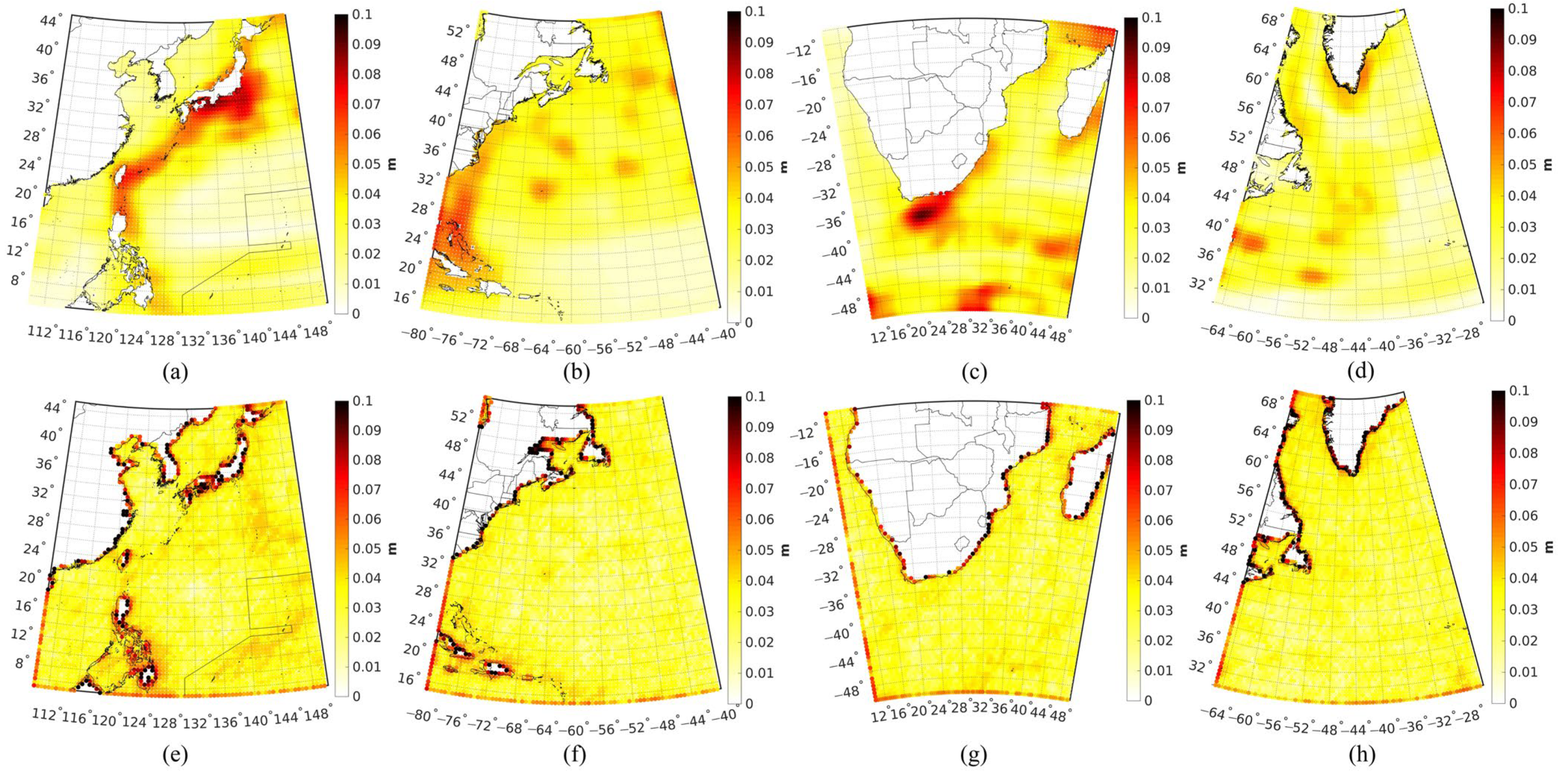
4.3. Formal Errors of the MDTs Estimated by MOA and LS Method

In the LS method and the MOA method, the MDT error can be calculated by Equation (8) and Equation (11), which can be seen in Figure 5. The formal errors of the LS-derived MDT (in the lower panel of Figure 5) were larger than those estimated by MOA method (in the top panel of Figure 5). The formal errors of the MOA-derived MDT ranged from a few millimeters to 10 cm, with an RMS value of about 3 cm. The formal errors of the LS-derived MDT ranged from about 1 cm to 20 cm, with an RMS value of about 3 cm. In the Kuroshio Current area, the errors of the MDT estimated by the LS method were large in the coastal area, by a magnitude of approximately 20 cm; while the formal errors of the MDT estimated by MOA method were less than 10 cm. The formal errors of the MOA-derived MDT for the southern coast of Japan were larger than for the eastern and southern coastal areas of China, by a magnitude of about 5 cm. The reason was that this region is located in the Kuroshio Current, and the formal errors of the MOA-derived MDT were mainly affected by the current. In the Gulf Current area, the formal errors of the LS-derived MDT were about 15 cm larger than errors of the MOA-derived MDT for the coastal area of North America, and about 20 cm larger than the errors of the coast of Canada. In the Agulhas Current area, the formal errors of the LS-derived MDT were about 15 cm larger than those of the MOA-derived MDT for the coastal area of Africa. In the Greenland Current area, the formal errors of the LS-derived MDT were larger than those of the MOA-derived MDT for the coast of Greenland, by a magnitude of about 20 cm. Moreover, the formal errors of MOA-derived MDT showed large values in ocean current area. Since the error of MSS reached decimeter level over coastal regions, the formal error of MDT computed from the MSS and geoid had at least the same magnitude of MSS’s error through error propagation. Thus, the formal errors of MDT estimated by the LS method may be more reasonable that those derived from the MOA method.
The formal errors of LS-derived MDT and the discrepancies between the estimated MDTs and ocean data (Figure 3) showed high consistency. Both showed larger differences over coastal areas. However, over ocean current areas, different structures could be found between them. The formal errors were relatively small where the discrepancies between the LS-derived MDTs and ocean data were obviously larger, see the structures in (72°W, 38°N) and (18°E, 38°S). The reason was that the error information of MSS we used may not have been accurate enough. In ocean current area, similar forms could be found between the formal errors of MOA-derived MDTs and the discrepancies between the MOA-derived MDTs and ocean data, but different patterns were displayed over coastal areas. The reason was that the variance and a priori error of MDT we used were not accurate, which were smaller than the values in other areas. The results showed that the formal error of the LS-derived MDT may have been more reasonable than that of the MOA-derived MDT.

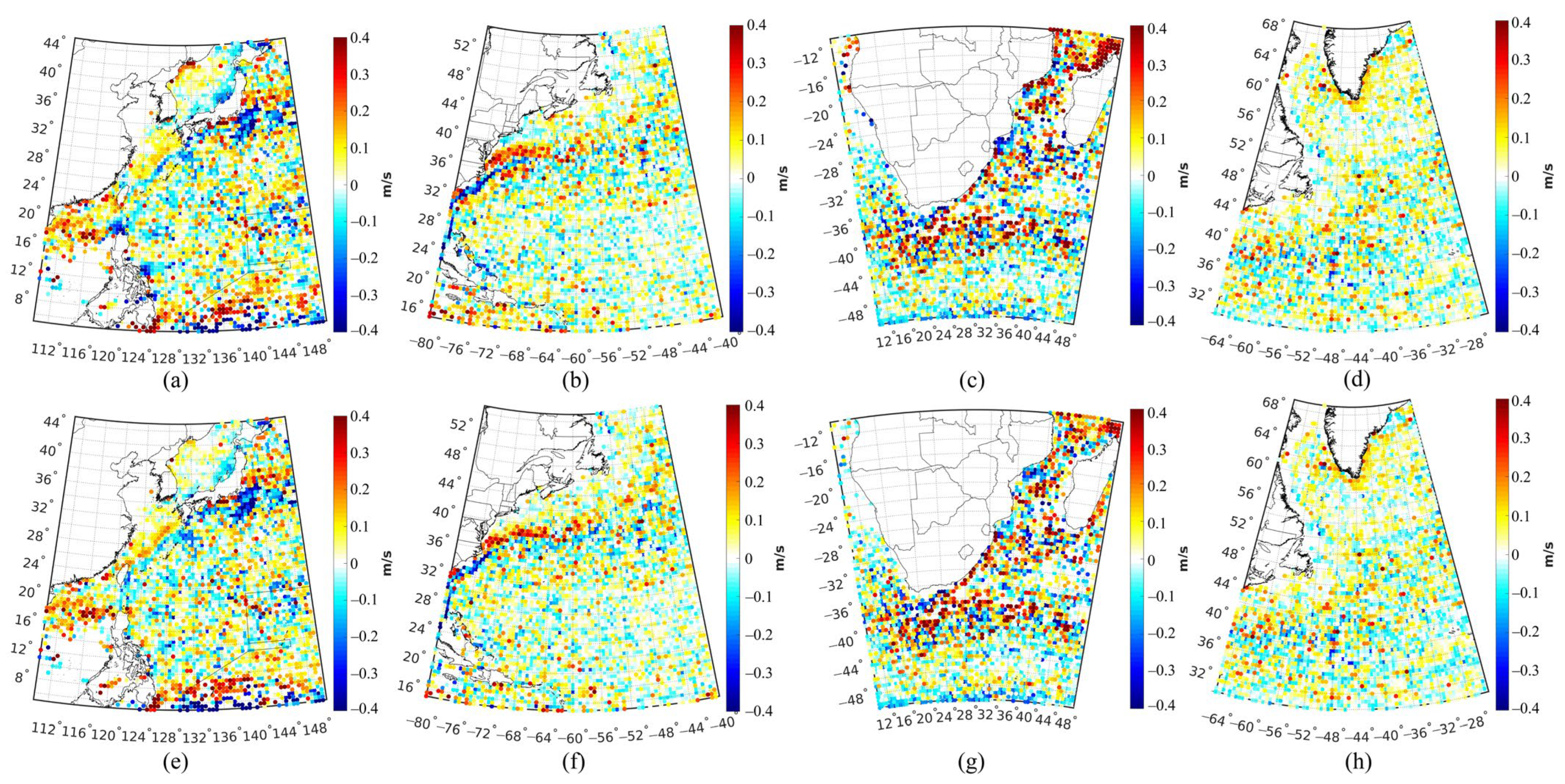
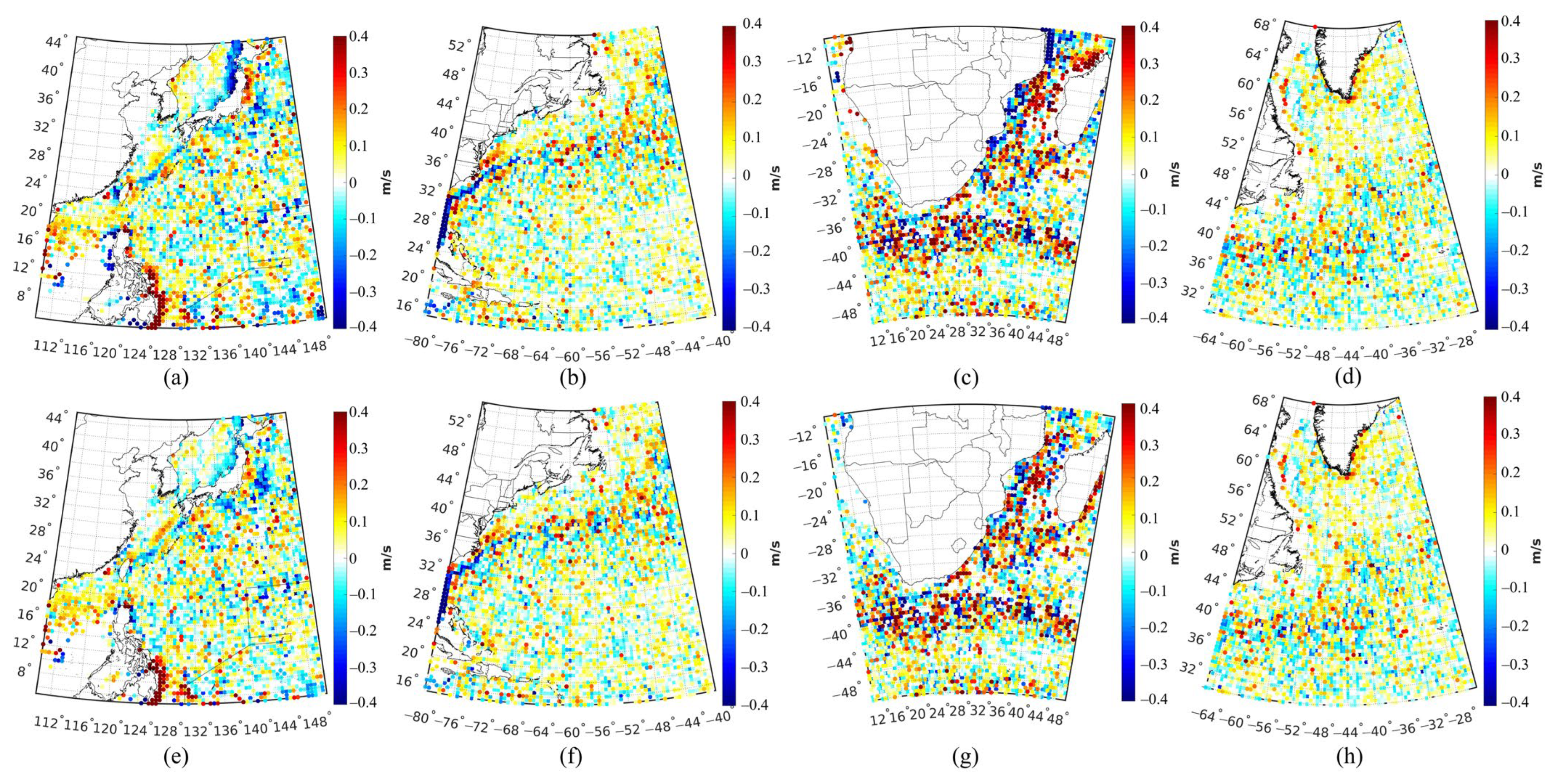
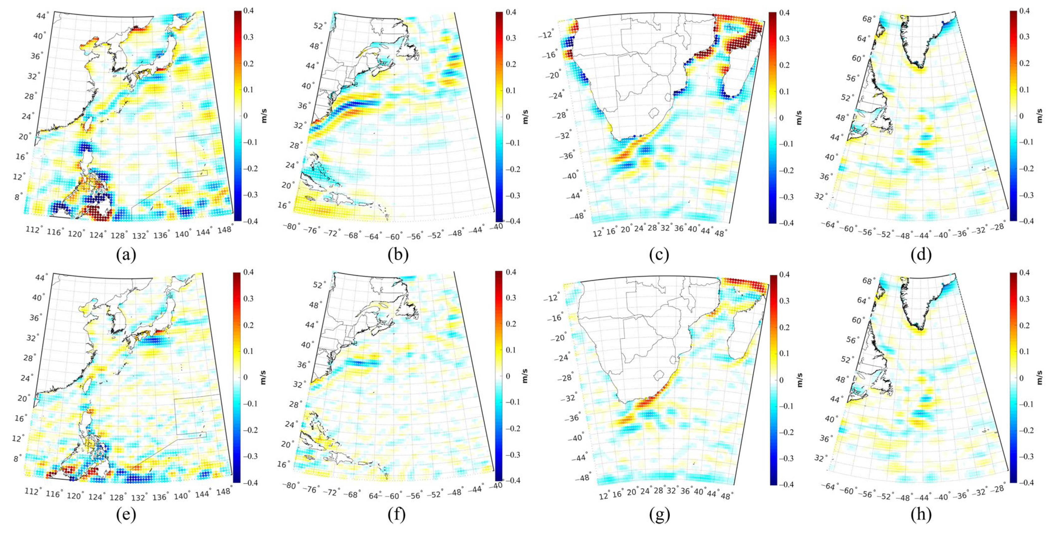
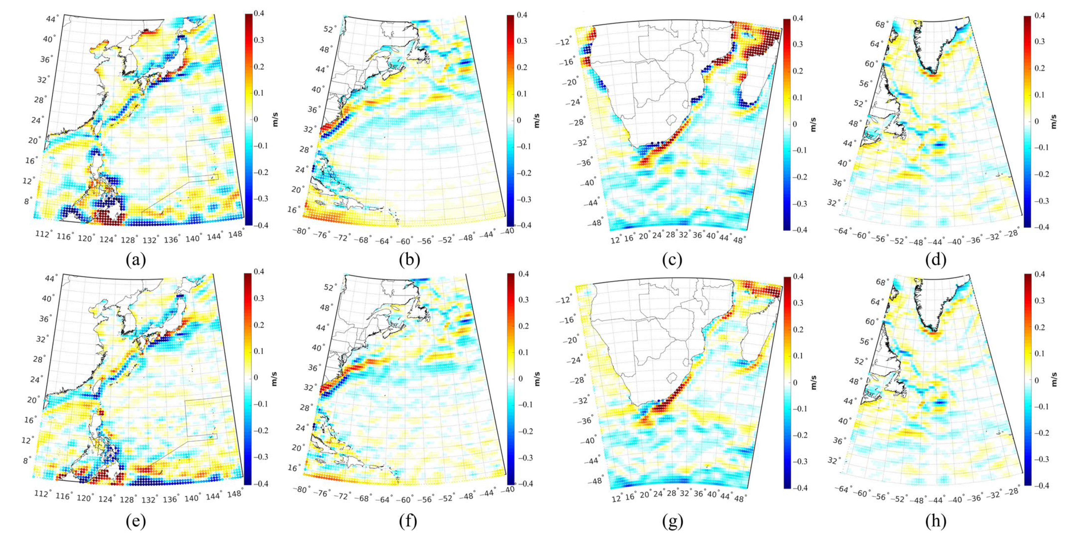
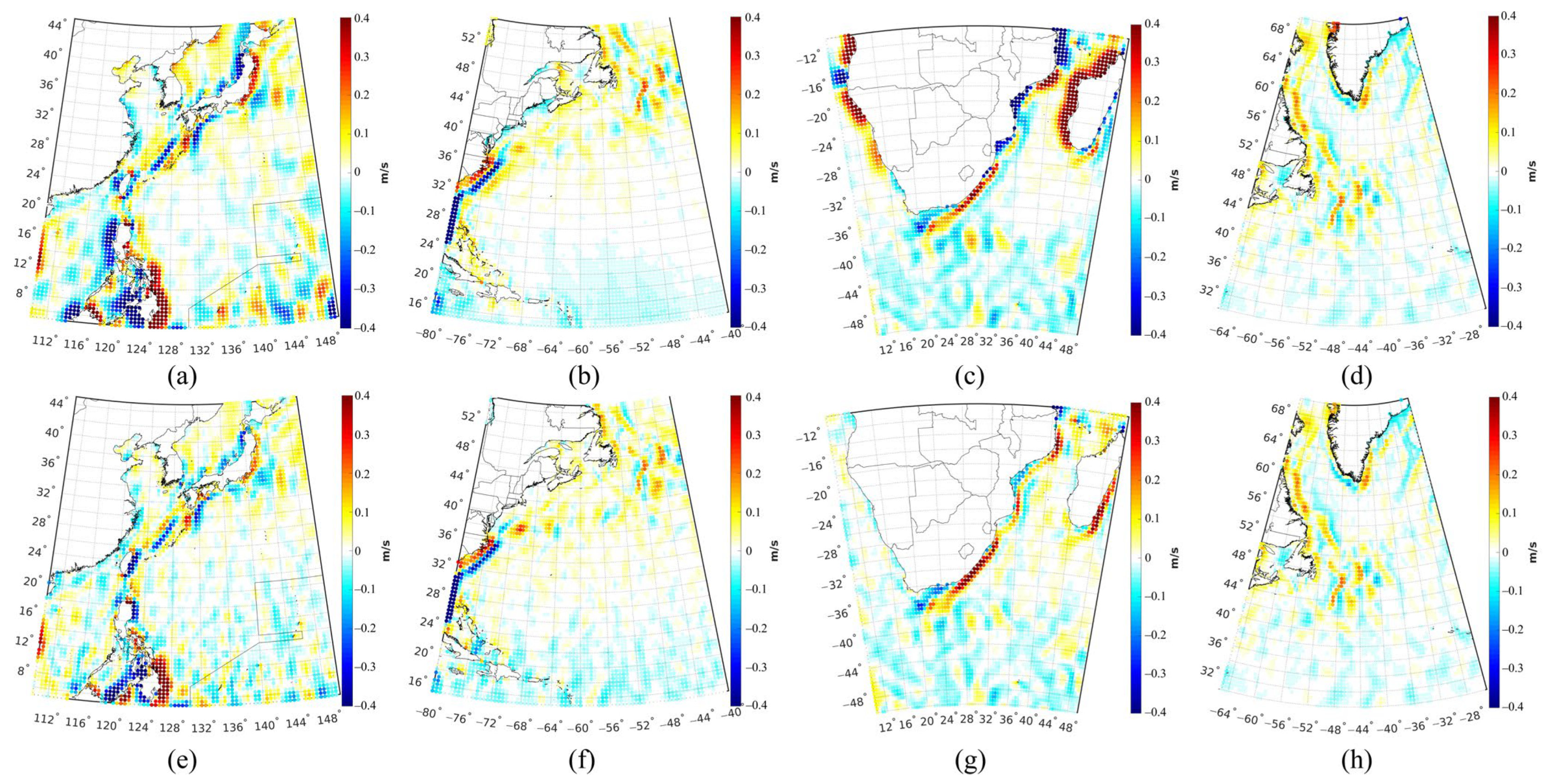
4.4. Comparison of Geostrophic Velocities Estimated by MDTs Derived from Different Methods

To further evaluate the MDT obtained by different methods, in situ buoy data were introduced as a reference in the form of geostrophic velocity [42]. The geostrophic velocities derived by estimated MDT were filtered by a Gaussian filter with a 60 km filter radius to make them smooth. The differences between the geostrophic velocities calculated by the MOA-derived (LS-derived) MDT and the buoy data are shown in Figure 6 and Figure 7. The LS-derived MDT had better fit with ocean data than the MOA-derived MDT. As for coastal areas, in the Kuroshio Current area, the discrepancies of geostrophic velocities between the LS-derived results and buoy data were clearly smaller than the MOA-derived results. For zonal geostrophic velocities, the discrepancies of geostrophic velocities between the LS-derived results and buoy data were about 2 cm/s smaller than that of the MOA-derived results for the coast of the Philippines. For meridian geostrophic velocities, the discrepancies of the LS-derived results were 2 cm/s smaller than the MOA-derived results for the coast of Japan. In the Gulf Current area, the discrepancies of geostrophic velocities between the LS-derived results and buoy data were clearly smaller than the MOA-derived results for the coasts of Canada and Cuba, by a magnitude of 3 cm/s. In the Agulhas Current area, the discrepancies of geostrophic velocities between the LS-derived results and buoy data were smaller than the MOA-derived results for the eastern and western coasts of Africa, by a magnitude of 3 cm/s. In the Greenland Current area, the discrepancies of geostrophic velocities between the LS-derived results and buoy data showed few discrepancies from that of the MOA-derived results. The reason was that there are several currents in the area, the sea states are complicated, and there were less buoy data than other areas, which may have resulted in inaccurate geostrophic velocity derived from buoy data. In addition, we have mentioned that the difference between the LS-derived MDT and the MOA-derived MDT was small.
As for ocean current areas, the discrepancies of geostrophic velocities between the LS-derived results and ocean data were slightly larger than the MOA-derived results, such as in the Gulf Current. The reason may have been because the sea surface state changes rapidly in the ocean current region, and the accuracy and resolution of buoy data were not high enough. As for open sea areas, the differences of geostrophic velocities between the LS-derived results and ocean data were similar to the MOA-derived results, which ranged from about −1.5 cm/s to 1.5 cm/s in the Kuroshio Current area, from −1 cm/s to 1 cm/s in the Gulf Current area, from −2 cm/s to 2 cm/s in the Agulhas Current area, and from −1 cm/s to 1.5 cm/s in the Greenland Current area.
The statistics of the discrepancies between the geostrophic velocities computed by the MDTs based on the different methods and buoy data are shown in Table 2. The RMSs of the discrepancies between the zonal (meridional) velocities calculated by LS-derived MDT and the buoy data were 0.4 cm/s (2.0 cm/s), 0.2 cm/s (0.3 cm/s) and 1.1 cm/s (2.3 cm/s) over the Kuroshio Current area, the Gulf Current area and the Agulhas Current area, respectively, which were lower than the velocities calculated by MOA-derived MDT. Meanwhile, the LS-derived MDT and the MOA-derived MDT had comparable performances for the Greenland Current area, as the RMSs of the discrepancies between the geostrophic velocities calculated by these two MDTs and the buoy data were 8.4 cm/s in zonal and 9.0 cm/s in meridional. These results indicated that the geostrophic velocity derived from LS-derived MDT outperformed that of MOA-derived MDT, especially in coastal and ocean current areas.

5. Discussion

The other MDT model and ocean models were applied to evaluate the MDT obtained by different methods. CNES-CLS18MDT was the reference model, which was modeled by combining the MSS model, geoid model, buoy data and hydrological profiles data. The differences between the geostrophic velocities calculated by the MOA-derived (LS-derived) MDT and those of CNES-CLS18MDT are shown in Figure 8 and Figure 9. The LS-derived MDT had better fit with the CNES-CLS18MDT than the MOA-derived MDT. As for coastal areas, in the Kuroshio Current area, the discrepancies of geostrophic velocities between the LS-derived results and buoy data were clearly smaller than those of the MOA-derived results. The discrepancies of geostrophic velocities between the LS-derived results and the CNES-CLS18MDT-derived results were about 10 cm/s smaller than those of the MOA-derived results for the coasts of the Philippines and Japan. In the Gulf Current area, the discrepancies of geostrophic velocities between the LS-derived results and the CNES-CLS18MDT-derived results were similar. In the Agulhas Current area, the discrepancies of geostrophic velocities between the LS-derived results and the CNES-CLS18MDT-derived results were smaller than those of the MOA-derived results in the eastern and western coasts of Africa, by a magnitude of 20 cm/s. In the Greenland Current area, the discrepancies of geostrophic velocities between the LS-derived results and the CNES-CLS18MDT-derived results showed few discrepancies from those of the MOA-derived results. For ocean current areas, the discrepancies of geostrophic velocities between the LS-derived results and the CNES-CLS18MDT-derived results were slightly larger than those of the MOA-derived results, such as in the Gulf Current. For open sea areas, the discrepancies of geostrophic velocities between the LS-derived results and the CNES-CLS18MDT-derived results were similar to those of the MOA-derived results. These results were similar to the results mentioned in Section 4.4.
The statistics of the discrepancies between the geostrophic velocities computed by the MDTs based on different methods and those of the CNES-CLS18MDT are shown in Table 3. The RMSs of the discrepancies between the zonal (meridional) velocities calculated by LS-derived MDT and the CNES-CLS18MDT were 3.8 cm/s (5.0 cm/s), 1.6 cm/s (0.7 cm/s), 6.1 cm/s (10.3 cm/s) and 0.2 cm/s (0.3 cm/s), over the Kuroshio Current area, the Gulf Current area, the Agulhas Current area and the Greenland Current area, respectively, which were lower than that of the velocities calculated by MOA-derived MDT. These results indicate that the geostrophic velocity derived from LS-derived MDT outperforms that of MOA-derived MDT, especially in coastal area and ocean current areas.
Moreover, the ocean reanalysis models, such as SODA, ORAS5 and Copernicus, which collect the geostrophic velocities data, were applied to evaluate the MDT obtained by different methods. In order to reduce the systematic error between the ocean reanalysis models, the mean of the three ocean reanalysis models was set as the reference data (called Ref-ocean-model in the following discussion). The differences between the geostrophic velocities calculated by the MOA-derived (LS-derived) MDT and the Ref-ocean-model are shown in Figure 10 and Figure 11. The geostrophic velocities derived by LS-derived MDT had better fit with the Ref-ocean-model than the MOA-derived MDT. As for coastal areas, the discrepancies of geostrophic velocities between the LS-derived results and Ref-ocean-model were mostly smaller than those of the MOA-derived results, especially for the coasts of the Philippines, Japan, and eastern and western coasts of Africa. For ocean current areas, the discrepancies of geostrophic velocities between the LS-derived results and the Ref-ocean-model were slightly larger than those of the MOA-derived results, such as in the Gulf Current. For open sea areas, the discrepancies of geostrophic velocities between the LS-derived results and the CNES-CLS18MDT-derived results were similar to those of the MOA-derived results. These results were similar with the results mentioned above, which indicated that the conclusion was not affected by the reference model.
The statistics of the discrepancies between the geostrophic velocities computed by the MDTs based on different methods and the Ref-ocean-model are shown in Table 4. The RMSs of the discrepancies between the zonal (meridional) velocities calculated by LS-derived MDT and the CNES-CLS18MDT were 3.1 cm/s (4.5 cm/s), 0.1 cm/s (0.5 cm/s), 4.9 cm/s (8.1 cm/s) and 0.2 cm/s (0.2 cm/s) over the Kuroshio Current area, Gulf Current area, Agulhas Current area and Greenland Current area, respectively, which were lower than the velocities calculated by MOA-derived MDT. These results indicated that the geostrophic velocity derived from LS-derived MDT outperformed that of MOA-derived MDT, especially in coastal and ocean current areas.

6. Conclusions

We focused on the comparison of methods of modeling MDT by using the multivariate objective analysis (MOA) method and rigorous least squares (LS) method. In particular, we evaluated the applicability of these two methods and compared their performances over different oceanic areas with different ocean state and hydrological conditions. Four local MDTs were computed, and the estimated MDTs were assessed by independent ocean data and buoy data. Moreover, the formal errors of the estimated MDTs based on these two methods were also analyzed and compared. The numerical results showed that:
(1)
The MDT derived from the LS method outperformed the MDT computed from the MOA method, especially over coastal areas and ocean current areas. The RMSs of the discrepancies between the LS-derived MDT and ocean data were 4.8 cm, 4.7 cm, 4.9 cm and 7.2 cm, for the Kuroshio Current area, Gulf Current area, Agulhas Current area and Greenland Current area, respectively, which were lower than those of the MOA-derived MDT, by a magnitude of 1.4 cm, 2.2 cm, 2.6 cm and −0.5 cm, respectively. The reason is that the LS method constructs the design matrix segmentally based on the error characteristics of the GGM, and then the signals are processed and constrained in different frequency bands to suppress high-frequency noise, which improves the quality of the estimated MDT;
(2)
The formal error of the MDT estimated by the LS method was more reasonable than that estimated by the MOA method. The errors of the MDT estimated by the LS method were prominent over coastal areas, which have larger magnitude, than estimated by the MOA method. The patterns of the formal errors of the LS-derived MDT were more realistic, since the errors of MSS models usually exceeded decimeter level along the coast, indicating the formal error of MDT computed from the MSS and geoid has at least the same magnitude of error as MSS, through error propagation;
(3)
Moreover, the geostrophic velocity derived from the LS-derived MDT was better than from the MOA-derived MDT, especially over coastal regions and ocean current areas. The RMSs of the discrepancies between the zonal (meridional) velocities calculated by the LS-derived MDT and the buoy data were 0.4 cm/s (2.0 cm/s), 0.2 cm/s (0.3 cm/s) and 1.1 cm/s (2.3 cm/s) smaller than of the velocities calculated by the MOA-derived MDT over the Kuroshio Current area, Gulf Current area and Agulhas Current area, respectively. The comparison between geostrophic velocities estimated by MDTs derived from different methods and the ocean models showed similar results. The results indicate that the LS-derived MDT outperforms the MOA-derived MDT.

Author Contributions

Conceptualization, Y.W. (Yihao Wu) and J.H.; methodology, Y.W. (Yihao Wu) and J.H.; software, J.H. and Y.W. (Yihao Wu); validation, Y.W. (Yihao Wu) and J.H.; formal analysis, Y.W. (Yihao Wu) and J.H.; investigation, Y.W. (Yihao Wu) and J.H.; resources, Y.W. (Yihao Wu); data curation, J.H.; writing—original draft preparation, Y.W. (Yihao Wu) and J.H.; writing—review and editing, Y.W. (Yihao Wu), X.H., H.W. and H.S.; visualization, J.H.; supervision, Y.W. (Yihao Wu), X.H. and H.W.; project administration, Y.W. (Yihao Wu); funding acquisition, Y.W. (Yihao Wu), X.H., H.W., Y.W. (Yunlong Wu) and Y.D. All authors have read and agreed to the published version of the manuscript.

Funding

This research was funded by the National Natural Science Foundation of China, grant numbers 42004008, 41830110, 41974016, 41974096 and 41931074; the Natural Science Foundation of Jiangsu Province, China, grant numbers BK20190498 and BK20190495; the Fundamental Research Funds for the Central Universities, grant numbers B220202055, B200202017 and B210201013; and the State Scholarship Fund from Chinese Scholarship Council, grant number 201306270014.

Data Availability Statement

The global geopotential models can be publicly accessed at http://icgem.gfz-potsdam.de/tom_longtime (accessed on 24 May 2022). DTU21MSS is available at https://ftp.space.dtu.dk/pub/ (accessed on 18 May 2022). CNES-CLS18MDT was accessed at ftp://ftp-access.aviso.altimetry.fr/auxiliary/mdt/mdt_cnes_cls2018_global (accessed on 16 May 2022). SODA3 was accessed at https://dsrs.atmos.umd.edu/DATA/soda3.12.2/REGRIDED/ocean/ (accessed on 18 May 2022). ORAS5 was accessed at https://icdc.cen.uni-hamburg.de/thredds/catalog/ftpthredds/EASYInit/oras5/ORCA025/catalog.html (accessed on 18 May 2022). Copernicus was accessed at https://cds.climate.copernicus.eu/cdsapp#!/dataset/satellite-sea-level-global?tab=overview (accessed on 20 May 2022). Drifter buoy data were accessed at https://www.aoml.noaa.gov/phod/gdp/index.php (accessed on 28 April 2022).

Acknowledgments

The authors would like to give their sincerest thanks to the anonymous reviewers for their constructive suggestions and comments, which were of great value for improving the manuscript. The authors also thank the editor for the kind assistances and beneficial comments. The authors are grateful for the kind support from the editorial office. We gratefully acknowledge the funders of this study.

Conflicts of Interest

The authors declare no conflict of interest.

References

  1. Filmer, M.S.; Hughes, C.W.; Woodworth, P.L.; Featherstone, W.E.; Bingham, R.J. Comparison between geodetic and oceanographic approaches to estimate mean dynamic topography for vertical datum unification: Evaluation at Australian tide gauges. J. Geod. 2018, 12, 1413–1437. [Google Scholar] [CrossRef] [Green Version]
  2. Chaigneau, A.A.; Reffray, G.; Voldoire, A.; Melet, A. IBI-CCS: A regional high-resolution model to simulate sea level in western Europe. Geosci. Model Dev. 2022, 5, 2035–2062. [Google Scholar] [CrossRef]
  3. Lin, H.; Thompson, K.R.; Huang, J.; Véronneau, M. Tilt of mean sea level along the Pacific coasts of North America and Japan. J. Geophys. Res. Oceans 2015, 120, 6815–6828. [Google Scholar] [CrossRef] [Green Version]
  4. Song, X. The importance of including sea surface current when estimating air–sea turbulent heat fluxes and wind stress in the Gulf Stream region. J. Atmos. Ocean. Tech. 2021, 1, 119–138. [Google Scholar] [CrossRef]
  5. Onink, V.; Wichmann, D.; Delandmeter, P.; van Sebille, E. The role of Ekman currents, geostrophy, and stokes drift in the accumulation of floating microplastic. J. Geophys. Res. Oceans 2019, 3, 1474–1490. [Google Scholar] [CrossRef] [Green Version]
  6. Wu, Y.; Abulaitijiang, A.; Featherstone, W.E.; McCubbine, J.C.; Andersen, O.B. Coastal gravity field refinement by combining airborne and ground-based data. J. Geod. 2019, 93, 2569–2584. [Google Scholar] [CrossRef]
  7. Wu, Y.; Huang, J.; Shi, H.; He, X. Mean Dynamic Topography Modeling Based on Optimal Interpolation from Satellite Gravimetry and Altimetry Data. Appl. Sci. 2021, 11, 5286. [Google Scholar] [CrossRef]
  8. Bingham, R.J.; Haines, K.; Hughes, C.W. Calculating the ocean’s mean dynamic topography from a mean sea surface and a geoid. J. Atmos. Ocean. Tech. 2008, 10, 1808–1822. [Google Scholar] [CrossRef] [Green Version]
  9. Knudsen, P.; Bingham, R.; Andersen, O.; Rio, M.H. A global mean dynamic topography and ocean circulation estimation using a preliminary GOCE gravity model. J. Geod. 2011, 85, 861–879. [Google Scholar] [CrossRef]
  10. Zhang, Z.; Lu, Y.; Hsu, H. Detecting surface geostrophic currents using wavelet filter from satellite geodesy. Sci. China Ser. D-Earth Sci. 2007, 50, 918–926. [Google Scholar] [CrossRef]
  11. Vianna, M.L.; Menezes, V.V.; Chambers, D.P. A high resolution satellite-only GRACE-based mean dynamic topography of the South Atlantic Ocean. Geophys. Res. Lett. 2007, 34, L24604. [Google Scholar] [CrossRef] [Green Version]
  12. Bingham, R.J.; Knudsen, P.; Andersen, O.; Pail, R. An initial estimate of the North Atlantic steady-state geostrophic circulation from GOCE. Geophys. Res. Lett. 2011, 38, L01606. [Google Scholar] [CrossRef] [Green Version]
  13. Becker, S.; Freiwald, G.; Losch, M.; Schuh, W.D. Rigorous Fusion of Gravity Field, Altimetry and Stationary Ocean Models. J. Geodyn. 2012, 60, 99–110. [Google Scholar] [CrossRef] [Green Version]
  14. Becker, S.; Brockmann, J.M.; Schuh, W.D. Mean Dynamic Topography Estimates Purely Based on GOCE Gravity Field Models and Altimetry. Geophys. Res. Lett. 2014, 41, 2063–2069. [Google Scholar] [CrossRef]
  15. Shi, H.; He, X.; Wu, Y.; Huang, J. The parameterization of mean dynamic topography based on the Lagrange basis functions. Adv. Space Res. 2020, 9, 2122–2140. [Google Scholar] [CrossRef]
  16. Rio, M.H.; Hernandez, F.A. Mean dynamic topography computed over the world ocean from altimetry, in situ measurements, and a geoid model. J. Geophys. Res. Oceans 2004, 109, C12032. [Google Scholar] [CrossRef] [Green Version]
  17. Rio, M.H.; Guinehut, S.; Larnicol, G. New CNES-CLS09 global mean dynamic topography computed from the combination of GRACE data, altimetry, and in situ measurements. J. Geophys. Res. Oceans 2011, 116, C07018. [Google Scholar] [CrossRef]
  18. Rio, M.-H.; Mulet, S.; Picot, N. Beyond GOCE for the ocean circulation estimate: Synergetic use of altimetry, gravimetry, and in situ data provides new insight into geostrophic and Ekman currents. Geophys. Res. Lett. 2014, 41, 8918–8925. [Google Scholar] [CrossRef]
  19. Lefèvre, F.; Lyard, F.H.; Le Provost, C. FES98: A new global tide finite element solution independent of altimetry. Geophys. Res. Lett. 2000, 17, 2717–2720. [Google Scholar] [CrossRef]
  20. Shi, H.; He, X.; Wu, Y.; Andersen, O.B.; Knudsen, P.; Liu, Y.; Zhang, Z. Spectrally Consistent Mean Dynamic Topography by Combining Mean Sea Surface and Global Geopotential Model Through a Least Squares-Based Approach. Front. Earth Sci. 2022, 10, 795935. [Google Scholar] [CrossRef]
  21. Wu, Y.; Huang, J.; He, X.; Luo, Z.; Wang, H. Coastal Mean Dynamic Topography Recovery Based on Multivariate Objective Analysis by Combining Data from Synthetic Aperture Radar Altimeter. Remote Sens. 2022, 14, 240. [Google Scholar] [CrossRef]
  22. Bretherton, F.P.; Davis, R.E.; Fandry, C.B. A technique for objective analysis and design of oceanographic experiments applied to MODE-73. Deep Sea Res. Oceanogr. Abstr. 1976, 23, 559–582. [Google Scholar] [CrossRef]
  23. Arhan, M.; De Verdiére, A.C. Dynamics of eddy motions in the eastern North Atlantic. J. Phys. Oceanogr. 1985, 15, 153–170. [Google Scholar] [CrossRef]
  24. Oka, E.; Kawabe, M. Dynamic Structure of the Kuroshio South of Kyushu in Relation to the Kuroshio Path Variations. J. Geophys. Res. 2003, 59, 595–608. [Google Scholar] [CrossRef]
  25. Oey, L.Y.; Ezer, T.; Forristall, G.; Cooper, C.; DiMarco, S.; Fan, S. An exercise in forecasting loop current and eddy frontal positions in the Gulf of Mexico. Geophys. Res. Lett. 2005, 12, L12611. [Google Scholar] [CrossRef] [Green Version]
  26. Franzese, A.M.; Hemming, S.R.; Goldstein, S.L.; Anderson, R.F. Reduced Agulhas Leakage during the Last Glacial Maximum inferred from an integrated provenance and flux study. Earth Planet. Sci. Lett. 2006, 1–2, 72–88. [Google Scholar] [CrossRef]
  27. Schlichtholz, P.; Houssais, M.N. An investigation of the dynamics of the East Greenland Current in Fram Strait based on a simple analytical model. J. Phys. Oceanogr. 1999, 29, 2240–2265. [Google Scholar] [CrossRef]
  28. Jiang, L.; Nielsen, K.; Dinardo, S.; Andersen, O.B.; Bauer-Gottwein, P. Evaluation of Sentinel-3 SRAL SAR altimetry over Chinese rivers. Remote Sens. Environ. 2020, 237, 111546. [Google Scholar] [CrossRef]
  29. Andersen, O.B.; Abulaitijiang, A.; Zhang, S.; Rose, S.K. A new high resolution Mean Sea Surface (DTU21MSS) for improved sea level monitoring. In Proceedings of the EGU General Assembly 2021, Göttingen Germany, 19–30 April 2021. EGU21-16084. [Google Scholar] [CrossRef]
  30. Förste, C.; Abrykosov, O.; Bruinsma, S.; Dahle, C.; König, R.; Lemoine, J.M. ESA’s Release 6 GOCE Gravity Field Model by Means of the Direct Approach Based on Improved Filtering of the Reprocessed Gradients of the Entire Mission; Data Publication; GFZ Data Services: Potsdam, Germany, 2019. [Google Scholar] [CrossRef]
  31. Carton, J.A.; Chepurin, G.A.; Chen, L. SODA3: A New Ocean Climate Reanalysis. J. Clim. 2018, 31, 6967–6983. [Google Scholar] [CrossRef]
  32. Zuo, H.; Balmaseda, M.A.; Tietsche, S.; Mogensen, K.; Mayer, M. The ECMWF operational ensemble reanalysis–analysis system for ocean and sea ice: A description of the system and assessment. Ocean Sci. 2019, 15, 779–808. [Google Scholar] [CrossRef] [Green Version]
  33. Mulet, S.; Rio, M.-H.; Etienne, H.; Artana, C.; Cancet, M.; Dibarboure, G.; Feng, H.; Husson, R.; Picot, N.; Provost, C.; et al. The new CNES-CLS18 global mean dynamic topography. Ocean Sci. 2021, 17, 789–808. [Google Scholar] [CrossRef]
  34. Mayer-Gürr, T.; Kvas, A.; Klinger, B.; Rieser, D.; Zehentner, N.; Pail, R. The combined satellite gravity field model GOCO05s. In Proceedings of the EGU General Assembly, Vienna, Austria, 12–17 April 2015. [Google Scholar]
  35. Bingham, R.J.; Haines, K. Mean dynamic topography: Intercomparisons and errors. Philos. Trans. R. Soc. A Math. Phys. Eng. Sci. 2006, 364, 903–916. [Google Scholar] [CrossRef]
  36. Ophaug, V.; Breili, K.; Gerlach, C. A comparative assessment of coastal mean dynamic topography in Norway by geodetic and ocean approaches. J. Geophys. Res. Oceans 2015, 120, 7807–7826. [Google Scholar] [CrossRef] [Green Version]
  37. Idžanović, M.; Ophaug, V.; Andersen, O.B. The coastal mean dynamic topography in Norway observed by CryoSat-2 and GOCE. Geophys. Res. Lett. 2017, 44, 5609–5617. [Google Scholar] [CrossRef] [Green Version]
  38. Wu, Y.; Abulaitijiang, A.; Andersen, O.B.; He, X.; Luo, Z.; Wang, H. Refinement of Mean Dynamic Topography Over Island Areas Using Airborne Gravimetry and Satellite Altimetry Data in the Northwestern South China Sea. J. Geophys. Res. Solid Earth 2021, 126, e2021JB021805. [Google Scholar] [CrossRef]
  39. Lumpkin, R.; Johnson, G.C. Global ocean surface velocities from drifters: Mean, variance, El Niño-Southern Oscillation response, and seasonal cycle. J. Geophys. Res. Oceans 2013, 118, 2992–3006. [Google Scholar] [CrossRef]
  40. Zingerle, P.; Pail, R.; Gruber, T.; Oikonomidou, X. The combined global gravity field model XGM2019e. J. Geod. 2020, 94, 66. [Google Scholar] [CrossRef]
  41. Lawson, C.L.; Hanson, R.J. Solving Least Squares Problems; Society for Industrial and Applied Mathematics: New York, NY, USA, 1995. [Google Scholar]
  42. Hwang, C.; Chen, S.A. Circulations and eddies over the South China Sea derived from TOPEX/Poseidon altimetry. J. Geophys. Res. Space Phys. 2000, 105, 23943–23965. [Google Scholar] [CrossRef]
Figure 1. The study areas: (a) Kuroshio Current area, (b) Gulf Current area, (c) Agulhas Current area, and (d) Greenland Current area. The red dashed lines represent the profiles, the blue lines represent the currents.
Remotesensing 14 05330 g001
Figure 2. The MDT estimated by MOA method in: (a) Kuroshio Current area, (b) Gulf Current area, (c) Agulhas Current area, and (d) Greenland Current area; and (eh) the MDT estimated by the LS method in the same respective areas.
Remotesensing 14 05330 g002
Figure 3. Differences between the estimated MDTs modeled by MOA method (top), LS method (below), and ocean data, in: (a,e) Kuroshio Current area, (b,f) Gulf Current area, (c,g) Agulhas Current area, and (d,h) Greenland Current area.
Remotesensing 14 05330 g003
Figure 4. Profiles of the discrepancies between the estimated MDTs and ocean data in: (a) Kuroshio Current area, (b) Gulf Current area, (c) Agulhas Current area, and (d) Greenland Current area. The blue (red) line represents the result of MOA (LS) method. Profiles 1, 2, 3 represent the results over coastal areas, open sea areas and ocean current areas, respectively.
Remotesensing 14 05330 g004
Figure 5. The formal errors of MOA-derived MDT (top) and LS-derived MDT (below), in: (a,e) Kuroshio Current area, (b,f) Gulf Current area, (c,g) Agulhas Current area, and (d,h) Greenland Current area.
Remotesensing 14 05330 g005
Figure 6. Discrepancies of the zonal geostrophic velocities between the values calculated by MDTs derived from different methods (top: MOA method; below: LS method) and buoy data in: (a,e) Kuroshio Current area, (b,f) Gulf Current area, (c,g) Agulhas Current area, and (d,h) Greenland Current area.
Remotesensing 14 05330 g006
Figure 7. Discrepancies of the meridian geostrophic velocities between the values calculated by MDTs derived from different methods (top: MOA method; below: LS method) and buoy data in: (a,e) Kuroshio Current area, (b,f) Gulf Current area, (c,g) Agulhas Current area, and (d,h) Greenland Current area.
Remotesensing 14 05330 g007
Figure 8. Discrepancies of the zonal geostrophic velocities between the values calculated by MDTs derived from different methods (top: MOA method; below: LS method) and that of CNES-CLS18MDT in: (a,e) Kuroshio Current area, (b,f) Gulf Current area, (c,g) Agulhas Current area, and (d,h) Greenland Current area.
Remotesensing 14 05330 g008
Figure 9. Discrepancies of the meridian geostrophic velocities between the values calculated by MDTs derived from different methods (top: MOA method, below: LS method) and that of CNES-CLS18MDT in: (a,e) Kuroshio Current area, (b,f) Gulf Current area, (c,g) Agulhas Current area, and (d,h) Greenland Current area.
Remotesensing 14 05330 g009
Figure 10. Discrepancies of the zonal geostrophic velocities between the values calculated by MDTs derived from different methods (top: MOA method, below: LS method) and the Ref-ocean-model in: (a,e) Kuroshio Current area, (b,f) Gulf Current area, (c,g) Agulhas Current area, and (d,h) Greenland Current area.
Remotesensing 14 05330 g010
Figure 11. Discrepancies of the meridian geostrophic velocities between the values calculated by MDTs derived from different methods (top: MOA method, below: LS method) and the Ref-ocean-model in: (a,e) Kuroshio Current area, (b,f) Gulf Current area, (c,g) Agulhas Current area, and (d,h) Greenland Current area.
Remotesensing 14 05330 g011
Table 1. Statistics of the discrepancies between MDT estimated by different methods and ocean data (units: cm; MOA: multivariate objective analysis; LS: least squares method).
AreaMethodMinMaxRMS
Kuroshio Current areaMOA−54.615.36.2
LS−42.433.64.8
Gulf Current areaMOA−75.440.46.9
LS−36.039.94.7
Agulhas Current areaMOA−59.759.67.5
LS−36.532.24.9
Greenland Current areaMOA−58.865.36.7
LS−29.828.97.2
Table 2. Statistics of the discrepancies between the geostrophic velocities computed from different MDTs based on different methods and buoy data (units: cm/s; u: zonal velocities; v: meridian velocities; MOA: multivariate objective analysis; LS: least squares method).
Study AreaMethodGeostrophic VelocitiesMinMaxRMS
Kuroshio Current areaMOAu−104.799.016.1
v−103.7169.115.4
LSu−116.675.115.7
v−98.995.013.4
Gulf Current areaMOAu−66.951.910.1
v−156.151.712.1
LSu−63.650.49.9
v−151.261.111.8
Agulhas Current areaMOAu−126.3110.919.7
v−171.8129.223.3
LSu−124.9113.318.6
v−119.0123.621.0
Greenland Current areaMOAu−77.548.68.4
v−58.768.69.0
LSu−77.548.68.4
v−58.768.69.0
Table 3. Statistics of the discrepancies between the geostrophic velocities computed from different MDTs based on different methods and that of CNES-CLS18MDT (units: cm/s; u: zonal velocities; v: meridian velocities; MOA: multivariate objective analysis; LS: least squares method).
Study AreaMethodGeostrophic VelocitiesMinMaxRMS
Kuroshio Current areaMOAu−95.8123.79.7
v−127.1115.410.9
LSu−45.374.75.9
v−54.648.95.9
Gulf Current areaMOAu−29.326.24.3
v−72.122.34.5
LSu−21.413.92.7
v−68.916.33.8
Agulhas Current areaMOAu−79.1140.210.7
v−176.1125.314.0
LSu−14.936.34.6
v−28.229.33.7
Greenland Current areaMOAu−26.114.62.9
v−29.626.42.7
LSu−19.712.62.7
v−12.215.82.4
Table 4. Statistics of the discrepancies between the geostrophic velocities computed from different MDTs based on different methods and the Ref-ocean-model (units: cm/s; u: zonal velocities; v: meridian velocities; MOA: multivariate objective analysis; LS: least squares method).
Study AreaMethodGeostrophic VelocitiesMinMaxRMS
Kuroshio Current areaMOAu−106.4151.512.2
v−133.7155.113.4
LSu−59.074.99.1
v−64.299.38.9
Gulf Current areaMOAu−60.733.55.4
v−108.033.07.2
LSu−67.133.65.3
v−96.741.26.7
Agulhas Current areaMOAu−77.2136.212.4
v−192.7121.715.0
LSu−29.259.67.5
v−58.352.96.9
Greenland Current areaMOAu−28.023.83.9
v−30.326.74.1
LSu−28.126.73.7
v−19.322.53.9
Publisher’s Note: MDPI stays neutral with regard to jurisdictional claims in published maps and institutional affiliations.

