Article

An Enhanced Spectral Fusion 3D CNN Model for Hyperspectral Image Classification

School of Mathematics and Computer Science, Wuhan Polytechnic University, Wuhan 430023, China
*
Author to whom correspondence should be addressed.
Remote Sens. 2022, 14(21), 5334; https://doi.org/10.3390/rs14215334
Submission received: 31 August 2022 / Revised: 19 October 2022 / Accepted: 20 October 2022 / Published: 25 October 2022
(This article belongs to the Special Issue Deep Learning for the Analysis of Multi-/Hyperspectral Images)

Abstract

:
With the continuous development of hyperspectral image technology and deep learning methods in recent years, an increasing number of hyperspectral image classification models have been proposed. However, due to the numerous spectral dimensions of hyperspectral images, most classification models suffer from issues such as breaking spectral continuity and poor learning of spectral information. In this paper, we propose a new classification model called the enhanced spectral fusion network (ESFNet), which contains two parts: an optimized multi-scale fused spectral attention module (FsSE) and a 3D convolutional neural network (3D CNN) based on the fusion of different spectral strides (SSFCNN). Specifically, after sampling the hyperspectral images, our model first implements the weighting of the spectral information through the FsSE module to obtain spectral data with a higher degree of information richness. Then, the weighted spectral data are fed into the SSFCNN to realize the effective learning of spectral features. The new model can maximize the retention of spectral continuity and enhance the spectral information while being able to better utilize the enhanced information to improve the model’s ability to learn hyperspectral image features, thus improving the classification accuracy of the model. Experiment results on the Indian Pines and Pavia University datasets demonstrated that our method outperforms other relevant baselines in terms of classification accuracy and generalization performance.

1. Introduction

In recent years, with the continuous development of hyperspectral image (HSI) technology [1], the analysis and processing of hyperspectral data has become one of the hotspots in many research areas [2]. HSIs are characterized by high information content, strong spectral continuity, high spectral resolution and so on. These characteristics allow HSIs to be used in an increasingly wide range of applications, such as environmental monitoring, agricultural production, mineral development and other fields [3,4,5]. Among the many applications of HSIs, the classification of pixels in images is one of the main research tasks [6].
HSI classification is more complex than traditional image classification to a certain extent. This is mainly reflected in two points: First, the number of HSIs is much smaller than the number of conventional images. Taking the COCO public dataset [7] as an example, it contains 91 easily recognizable object categories with a total of 2.5 million tagged instances in 328,000 images. The common public dataset of HSIs generally has only one original dataset containing spectral data and label data. Second, the spectral dimension of an HSI is much larger than that of a traditional image. The large amount of spectral data makes it difficult for general classifiers to achieve high accuracy, especially when the training samples are extremely limited. Therefore, HSI classification can be studied from two aspects: classification and spectral information processing.
Early researchers faced with the problem of how to deal with complex spectral information mainly processed spectral information via the following methods: principal component analysis (PCA), independent component analysis (ICA), linear discriminant analysis (LDA), etc. The key point of these methods is to select the most representative and effective spectra and discard some spectra that do not contribute much to the classification in order to achieve dimensionality reduction of HSIs. However, the biggest problem with these methods of processing HSIs is that the spectral information of HSIs is very typical of nonlinear relationships, while PCA and LDA are traditional linear processing methods [8]. Therefore, it is not robust to process the spectral information of HSIs by these linear methods. As for HSI classification, the early methods are mainly based on machine learning methods. For example, support vector machines (SVM) [9], the k-nearest neighbor algorithm (k-NN) [10] and the naive Bayesian algorithm [11] are used for classification of HSIs. In the face of hyperspectral images with few labeled samples, Zhang et al. [12] proposes a semisupervised classification method based on simple linear iterative cluster (SLIC) segmentation for HSIs. However, in the processing of features by traditional machine learning methods, compared with deep learning methods, deep learning methods can extract higher-level features [13]. Therefore, researchers have started to solve HSI classification and spectral information processing by using deep learning methods.
Compared with traditional machine learning methods, deep learning methods can automatically extract features from each layer and train the classification model at the same time. With the increase in the number of layers, the overall model will continue to become more robust [14]. As a result, deep learning methods have become increasingly popular in recent years [15,16], especially in the field of image processing [17,18,19,20,21]. In the face of evolving HSI technology, Chen et al. [22] applied deep learning methods to HSI classification for the first time. Since then, there have been an increasing number of HSI studies based on deep learning [23,24]. The research targeting HSI classification can be divided into two main lines:
(1)
HSI [25]. Due to the rich spectral information and continuity of HSIs, the rich spectral information cannot be handled well or effectively by traditional dimensionality reduction methods. Luo et al. [26]. proposed a multi-structure unified discriminative embedding method to better represent the low-dimensional features of HSIs. With the proposal of the SE module [27], the attention mechanism has received more and more attention. The biggest advantage of the attention mechanism is that it can focus on the useful channel information when facing multiple channels and can directly establish the dependency between input and output, which enhances the parallelization of models [28]. It is an effective attempt to introduce an attention mechanism into his classification. The spectral information of HSIs can be effectively enhanced by weighting each band of HSIs through the channel attention mechanism. Ma et al. [29] went further on this basis and proposed an attention mechanism module using the correlation between spectra obtained by multi-scale convolution, the SeKG module, which further enhanced the spectral information.
(2)
HSI classification models [23]. Due to the large number of classification models based on deep learning methods, the study of classification models is one of the research hotspots for HSI classification. Chen et al. [30] used a deep belief network (DBN) to extract features and classify HSIs. Mou et al. [31] used recurrent neural networks (RNN) to achieve classification of HSIs. In the last decade of research on deep learning-based classification models, convolutional neural networks (CNNs) have emerged as one of the main focuses in the research field due to their advantages of feature extraction through local connectivity and weight sharing to reduce the number of parameters. For HSI classification, Zhao et al. [32] first used PCA to reduce the dimension of the original HSI and then extracted features from the reduced image using a CNN model to achieve the classification of the HSI. Zhang et al. [33] input HSIs of different regions into a CNN, expecting better classification results. Guo et al. [34] proposed a CNN-based spatial feature fusion model that can fuse spatial information into spectral information to obtain good classification results. In recent years, other methods used to study hyperspectral image classification using convolutional neural networks or other deep learning methods are FusionNet [35], HSI bidirectional encoder representation from transformers (HSI-BERT) [36], spatial–spectral transformers (SST) [37] and two-stream spectral-spatial residual networks (TSRN) [38]. With the CNN model being studied for a long time, the 3D CNN model was proposed by Tran et al. [39]. The biggest advantage of 3D CNN over 2D CNN is that the features of the channel dimension can be extracted, which is very suitable for HSIs. Chen et al. [40] applied 3D CNN to the classification of HSIs. After that, many researchers have begun using 3D CNN for HSI classification. For example, Ahmad et al. [41] proposed a 3D CNN model that can rapidly classify hyperspectral images. Zhong et al. [42] designed a residual module based on 3D CNN to extract spatial and spectral information and applied it to HSI classification. Laban et al. [43] proposed a 3D deep learning framework which combined PCA and 3D CNN. Due to the advantages of 3D convolution, other models for hyperspectral image study using 3D CNN are: spectral four-branch multi-scale networks (SFBMSN) [44], 3D × 2D CNN [45] and 3D ResNet50 [46]. However, as 3D CNN has the ability to extract both spatial and spectral information, there is no need to extract spatial and spectral features separately.
By analyzing these two main lines, we can find some new ideas or problems that can be solved: (1) Can the two main lines of research be better integrated? Although research on HSIs serves classification models, ordinary classification models are not effective in extracting the main features of the spectra due to the complexity of the original spectral information of hyperspectral images. So, can we design a network structure that can better learn the spectral features after processing? (2) In terms of classification models, 3D CNN is theoretically well suited to HSIs. It is worthwhile to try to make the design idea of the new network structure more closely fit 3D CNN.
In order to solve the above problems, we designed and tested a new HSI classification model (ESFNet). The innovations of our model can be divided into two parts:
(1)
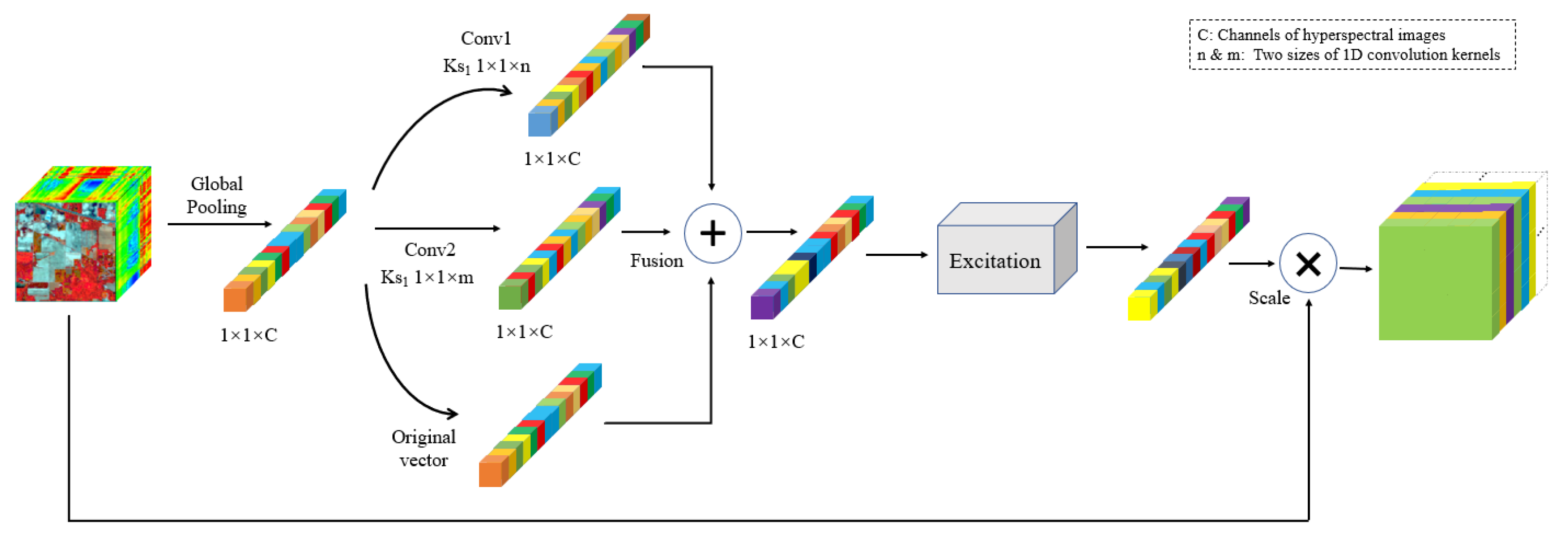
We optimize the SeKG module [29], termed FsSE. In order to better process and utilize the spectral information while preserving the continuity between spectra as much as possible, we reduce the convolution of multiple scales in the SeKG module to two scales and set the scaling parameter in the excitation layer to 1. These two optimizations allow the module to extract correlations between spectra more efficiently while retaining maximum spectral continuity, so that the classification model can better learn the spectral features.
(2)
We propose a new network named the spectral stride fusion network (SSFCNN). The new network implements the fusion of different strides by taking advantage of the fact that 3D CNN can slide in the spectral dimension. This structure not only enhances the learning ability of the model regarding spectral features, but also solves the problem of redundant spectra.
Our model effectively solves the problem of integrating the two main lines mentioned above. On the one hand, the usefulness of the FsSE module cannot be realized if the enhanced information of this module is not effectively utilized. On the other hand, without the support of enhanced features, the advantages of SSFCNN cannot be better demonstrated. Therefore, the two parts are complementary and indispensable, which greatly enhances the model’s ability to learn spectral characteristics. A series of experiments shows that our proposed ESFNet is effective, and its overall accuracy is better than that of other classification models.
The rest of the paper is organized as follows. Section 2 introduces the FsSE module and SSFCNN. Section 3 presents the datasets used for the experiments, the experimental environment and the training and test sets. Section 4 focuses on the relevant experimental analysis. Finally, conclusions and discussions are summarized in Section 5.

2. Enhanced Spectral Fusion Network (ESFNet)

2.1. FsSE Module

Because hyperspectral images (HSI) have hundreds of spectral bands, traditional hyperspectral processing methods generally begin with dimensionality reduction methods such as PCA before employing HSI classification methods such as neural networks. One obvious problem with these methods is that the number of spectral bands reserved needs to be determined subjectively, which will prevent the most efficient use of spectral information. However, if training is directly input into the neural network without dimension reduction, there will be a problem, in that the spectral characteristics cannot be well learned. Thus, it is a good solution to adaptively adjust the weights of spectral channels by introducing a channel attention mechanism to enhance and suppress different channels so that the classification model can better learn the spectral features.
We were inspired by SENet [27] and SSKNet [29]. In order to effectively extract the features of different spectral bands of different grounds, we optimized the SeKG module in SSKNet and named the optimized module the two-scale fusion SE module (FsSE module). Figure 1 shows the structure of this module.
In the SE module, the input data are compressed into a one-dimensional tensor by global averaging pooling, and then the exclusive mask of the channel is obtained through the excitation layer to achieve weighting of the channel. However, this strategy has a drawback for HSIs: it ignores a certain correlation that exists between HSI spectra. Therefore, it is necessary to improve the specificity of HSIs. In SSKNet, the SeKG module first performs multiscale convolution on the one-dimensional tensor obtained by global averaging pooling and then fuses the convolved results. Finally, the weight of the channel is obtained through the same excitation as in SENet. Based on the SE module, the SeKG module proposes multi-scale convolution for the spectra of an HSI to extract the correlation of the spectra at different distances. In the SeKG module, Ma et al. defined a set of multi-scale convolution kernels f = [ f 1 ,   f 2 , ,   f k ] , which can be used to extract the spectral correlation at multiple distances. Our experiment shows that this multi-scale convolution strategy is sufficient to extract spectral correlations using only two scales, and the distance between scales should not be too large. Meanwhile, in order to retain as much spectral continuity as possible, we set the scaling parameter in the excitation module to 1. We will introduce the implementation process in detail below.
The input of the model is hyperspectral data X h × w × c , h and w are the length and width of the input data, respectively, and c is the number of spectral bands. After global averaging pooling, a one-dimensional spectral channel vector X c = { X 1 ,   X 2 , ,   X c } can be obtained. The formula can be expressed as:
X l = i = 1 h j = 1 w X l ( i , j ) h × w , l = ( 1 , 2 , 3 , , c )
After obtaining one-dimensional spectral channel vectors, we use multiscale convolution to weigh the spectral characteristics to enhance the correlation between the spectra.
We only set up two convolution cores of different scales K s = { K s 1 ,   K s 2 } . The layer is a 1D convolution, and the size of the convolution kernel is 1 × 1 × c k ,   c k = { 3 ,   5 ,   7 , } . The size of the convolution kernel can be adjusted according to the experiment. The convolution kernel slides in the direction of the spectral dimension, and the stride length is 1. The value generated by the convolution represents the correlation between the spectra at that size. The size after convolution is ensured to be the same as the original size by zero-padding. Finally, we used the ReLU function to ensure that the channel correlation is positive. The specific calculation formula is as follows:
{ Y l = i = 0 c k 1 X l + i K s i + 1 + b , l = ( 1 , 2 , 3 , , c ) X l + i = 0 , l + i > c
where Y c = { Y 1 ,   Y 2 , ,   Y c } represents the result after convolution, and the size of the output is still 1 × 1 × c , as we only use two scales Y c = { Y 1 ,   Y 2 } . b represents the bias value. In order to obtain a wealth of spectral information, we fused the results of the obtained spectral correlations at different convolution scales by channel. This can be expressed in a formula as:
F s = X c Y 1 Y 2
F s represents the spectral features after fusion. X c represents the original one-dimensional spectral channel vector. Y 1 and Y 2 represent the results obtained at two convolution scales. represents the summation of these three vectors. Each channel of the fused feature contains the original spectral information and the related features of the adjacent spectrum, which can better generate channel weights that match the HSI.
In order to obtain the mask of the spectral channels, we need to input the fused results into an excitation module consisting of two fully connected layers. In the SE module and SeKG module, in order to reduce the amount of computation, the first fully connected layer usually reduces the dimensionality of the data to c / r (c represents the number of channels, while r represents the scaling parameter). The second fully connected layer restores the dimensions to the original dimensions. This processing is a good choice for ordinary images. However, for HSIs, the wealth of spectral information is the biggest characteristic. In addition, we further enriched the spectral information by multi-scale fusion. The method to reduce the dimension before restoring it will undoubtedly cause part of this rich information to be lost. Therefore, we used a fully connected layer with the same number of nodes in both layers (i.e., the scaling parameter is set to 1), which not only reduces the effectiveness of this module but also preserves the spectral information. The formula for calculating the channel mask can be expressed as
M = ( ( L 2 ( L 1 F s ) ) )
In Formula (4), represents the sigmoid function. represents the ReLU function. L i represents the fully connected layer. After obtaining the final channel weights M, the weighted result is obtained by multiplying M with the two-dimensional matrix input to the module through the scale operation.
By this step, the correlation problem between multiple spectra is alleviated, and the subsequent classification model is facilitated to learn more spectral features.

2.2. Spectral Stride Fusion Network (SSFCNN)

2.2.1. 3D Convolution

The biggest difference of 3D CNN compared to 2D CNN is that the kernel can slide on the channels. For input data with a large number of channels, a 3D CNN model can learn more abundant features, which perfectly fits the characteristics of HSIs. Thus, 3D CNN can take full advantage of the rich spectral information of HSIs and learn richer spectral features by sliding over the spectral dimension by using 3D kernels. Figure 2 shows 2D convolution and 3D convolution.
In 3D CNN, the calculation formula of the output O x y z value of the neuron node (x, y, z) is as follows:
O x y z = i = 0 K w 1 j = 0 K h 1 m = 0 K c 1 I ( x + i ) ( y + j ) ( z + m ) K ( i + 1 ) ( j + 1 ) ( m + 1 ) + b
In Formula (5), K w , K h and K c represent the width, height and number of channels of the kernel, respectively. I x y z is the input, and b is the bias value.

2.2.2. SSFCNN

HSIs are rich in spectral information. In order to make better use of this important characteristic, we designed a 3D CNN model based on spectral feature fusion named the spectral stride fusion network (SSFCNN). The structure we designed can both ensure that enough spectral information is collected and make the model learn more abundant features by fusing different spectral information. The reason why we want to emphasize the learning ability of the model for spectral features is that in an actual HSI, there are certain similarities between the spectra of different ground objects. Taking the Indian Pines dataset as an example, we plotted the spectral curves of these 16 types of samples. From Figure 3, we can see that the trend of the spectral curves of these 16 types of samples is basically the same and has strong continuity. This requires the model to have a stronger spectral learning capability. Therefore, our original intention of designing SSFCNN is to solve this problem.
Compared with the traditional HSI classification model using a convolutional neural network, a 3D convolutional neural network (3D CNN) can classify images relatively quickly without manual dimensionality reduction. The difference between the method in this paper and the general 3D CNN model is that the structure we designed allows the model to extract spectral features under different spectral strides and then fuse those features. This structure allows for both dimensionality reduction and for the network to learn different spectral features, which can better guide the model to classify targets. Figure 4 shows the network structure of our model.
Taking the Indian Pines dataset as an example, through Figure 4, we aimed to fuse the results of two different spectral strides. The values of stride for each layer are (1, 3) and (1, 5), respectively. The results of the two different strides are concatenated by the concat operation. We use different spectral sampling strides for concatenation because the spectral features extract at different strides are not the same. With a small stride, the model can extract more spectral features, but it also extracts some redundant information; with a large stride, the model extracts less redundant information, but the wealth of the spectral features is likewise reduced. As a result, we planned to combine the results at different stages so that they could complement each other. With the extraction of the two strides, the model can learn more abundant spectral information. The first two layers of the model are designed according to this idea. In Layer3, in order to facilitate the final model output, the fusion strategy is no longer used. However, the size of the feature map arriving at Layer3 will be different due to the size of the patch. When the patch size is less than 9, the size of the feature map reaching that layer is already a one-dimensional vector, and there is no need to downsample the feature map. Therefore, we set a discriminator to judge the feature maps input to Layer3. Finally, the final output is calculated through the fully connected layer.

3. Experimental Setting

3.1. Dataset

Two public datasets, the Indian Pines dataset and the Pavia University dataset, were used in this experiment. The Indian Pines dataset was collected by the Airborne Visible/Infrared Imaging Spectrometer (AVIRIS) sensor over Northwest Indiana, United States, in 1992. This dataset consists of 145 × 145 pixels with a spatial resolution of 20 m. There are 220 continuous bands in the wavelength range of 400~2500 nm, with 20 water absorption and low signal-to-noise ratio bands (104~108, 150~163, 220) removed. The ground truth includes 16 types of samples, most of which are crops at different growth stages. The spectral features of these 16 types of samples are relatively similar, and the image resolution is low, which can easily produce mixed hybrid pixels, thus causing some difficulties in image classification. Figure 5 shows the pseudo-color image and the ground truth, respectively.
Figure 6 shows the Pavia University dataset. This dataset was acquired in 2002 using ROSIS sensors over Pavia, Italy. It includes nine types of samples, such as roads, numbers and roofs. The image consists of 610 × 340 pixels with a spatial resolution of 1.3 m. There are 115 bands in the wavelength range of 430~860 nm, of which 103 bands are reserved for testing after removing 12 bands with strong noise and water absorption.

3.2. Running Environment

The processor used for the experiments is an i7-10750H from Intel with a main frequency of 2.60 GHz. The graphics card used for the experiments is an RTX2060 from NVIDIA with 6 GB of video memory. The experimental device has 16 GB of memory. The system used is Windows 10. The deep learning framework used is Pytorch.

3.3. Dataset Processing

In this paper, a fully supervised learning approach is used, and the dataset is divided into the training set and the test set. Figure 7 shows the training set and test set of two datasets.

4. Discussion

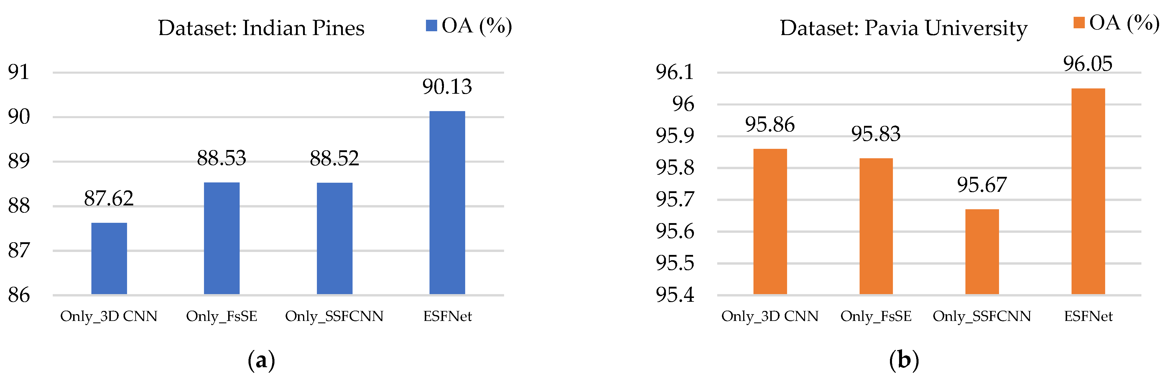
4.1. Comparison of Modules

To be able to further illustrate that the combination of both the FsSE module and the classification model SSFCNN can significantly improve the overall accuracy of the model, we conducted three sets of comparison experiments. The three sets of comparison experiments were modeled as follows: (1) a simple 3D CNN model without using the FsSE module and SSFCNN; (2) a simple 3D CNN model that only makes use of the FsSE module; and (3) SSFCNN without using the FsSE module. Figure 8 shows the accuracies of the four models.
In Figure 8, we can clearly see that the effect of ESFNet is better than the other three groups of comparison experimental models. We know that the FsSE module enhances the information contained in each band of the hyperspectral image (HSI), but the global averaging pooling in the FsSE module obtains a global receptive field and does not take into account the spatial information. SSFCNN has the capability of spatial learning while enhancing the learning ability of spectra, but if the classification model is allowed to learn the original spectral bands directly, the effective band information cannot be extracted efficiently. In the results shown in Figure 8, the accuracy only has a little difference when either method is used alone. However, after combining FsSE with SSFCNN, the accuracy of prediction can be significantly improved. The reason why the combined model can improve the accuracy is that it can both ensure the continuity of the HSI spectra and enhance the spectral information of the HSI while allowing the enhanced information to be better utilized in the classification model. Therefore, our idea of designing this new classification model for HSIs is effective.

4.2. Parameter Sensitivity Analysis

Some hyperparameter settings in the ESFNet module can have an impact on the effect of the model. After analysis, we mainly analyze the performance of the model from three aspects: the size of the convolution kernel in the FsSE module, the combination of strides in SSFCNN and the patch size of the input. We set the batch size to 16, used the RMSprop algorithm as the optimizer of the loss function and set the epoch of all models to 200. The test set is evaluated by selecting the model with the highest detection accuracy on the validation set, and finally the best choice of these three components is used as the final choice of the model, which is compared with other models in Section 4.3. It should be noted that the other parameters of the model are the same when we analyze a particular parameter.

4.2.1. Impact of Convolution Kernel Size of the FsSE Module on Model Accuracy

We will introduce the advantages of this module in Section 3. However, due to the different settings of the convolution kernel size, the extracted spectral correlations are different. Common convolution kernels are typically of size 3, 5 or 7. Therefore, we conducted three sets of comparison experiments for both datasets. Figure 9 shows the results.
From Figure 9, it can be seen that for extracting the correlation between the spectra, a high accuracy has been achieved by using the convolution of two scales. Because of the strong continuity existing between spectra, the use of two convolution kernels with little difference in size is enough to ensure that the model can extract sufficient spectral correlation. Therefore, our optimization of the SeKG module is effective. The best combination of convolution kernels for the Indian Pines dataset is 1 × 1 × 5 and 1 × 1 × 7 because the model has the highest accuracy with this combination. For the Pavia University dataset, the accuracy of the convolution kernel combinations 1 × 1 × 3 & 1 × 1 × 7 and 1 × 1 × 5 & 1 × 1 × 7 is the same. Thus, we need to analyze these three combinations from other perspectives. Table 1 shows the training time and the number of parameters for the three combinations on the Pavia University dataset.
From Table 1, it is obvious that the combination 5&7 takes the least time to train among the three combinations. Although the number of parameters is the largest among the three, the number of extra parameters is very small. Therefore, in the case that the two combinations of 3&7 and 5&7 have the same accuracy for the Pavia University dataset, the less time-consuming combination of 1 × 1 × 5 and 1 × 1 × 7 is chosen.

4.2.2. Impact of Patch Size on Model Accuracy

Because the image in the public hyperspectral dataset is only one piece, if the whole image is input into the network for training, it is not only disadvantageous for the network training, but also the amount of data is far from enough. Therefore, we need to sample the image and send the sampled part into the network for training, which can both reduce the training time of the model and increase the training volume of the model. Taking the Indian Pines dataset as an example, the size of the original image is 145 × 145 × 200, and we select a block of M × M × 200 pixels to input into the model for training. The choice of patch size, however, can have a significant impact on model accuracy and training time as well. If the selected size is too small, the model will not be trained properly; if the selected size is too large, the model training time will increase. Therefore, in order to select the best patch size, we chose seven different sizes of sampling windows for comparison. Figure 10 shows the accuracy for the two datasets when faced with different patch sizes.
From Figure 10a, we can observe that the model has the highest accuracy in classifying the Indian Pines dataset when the size of the sampling is increased to 11, and then the accuracy decreases as the patch size increases. From Figure 10b, we can see that the accuracy of the model is highest when the patch size is 5. After that, the accuracy of the model on the Pavia University dataset decreases when the patch size continues to increase. Also, we know that the patch size not only affects the accuracy of the model, but also has an impact on the training time of the model. Table 2 shows the training time of the model with seven patch sizes.
Table 2 clearly shows the relationship between the training time and the patch size. With increasing size, the training time increases as well. For the Pavia University dataset, a patch size of 5 gives the best results and takes the least amount of time to train. For the Indian Pines dataset, although the training time is at its minimum when the patch size is set to 5, the accuracy is 7.296% lower than when the size is 11. Therefore, for the Indian Pines dataset, a patch size setting of 11 is optimal.

4.2.3. Impact of Stride Combinations on Model Accuracy

We already know that there is a certain degree of redundant information in the spectra of an HSI, which is the theoretical basis for the use of descending dimension methods such as PCA in numerous studies of HSI classification. In the same way, even if we weight the spectral information by the set FsSE module, the redundant information still exists, which requires us to find ways to make the 3D CNN model learn as much effective information as possible. Therefore, we designed SSFCNN to solve this problem. However, with different spectral strides, the extracted spectral features are different. To study the effect of this part on the model, we set up multiple combinations. Table 3 and Table 4 show the accuracy and training time of these combinations on the two datasets.
From Table 3, the combination of Layer1 and Layer2 of the model is 1_3 and 1_5. The model has the best classification effect on the Indian Pines dataset, and the accuracy rate is generally 1%–2% higher compared with other combinations. Although the training time is a bit higher than for other combinations, it is still within an acceptable range. The accuracy on the Pavia University dataset can be analyzed by Table 4. It can be seen that the accuracies of different combinations are close. Figure 11 shows the accuracies more visually.
From the training time, when the combination is 1_7 and 1_5, the training time is the second lowest among all combinations, and the accuracy is also the highest. However, due to the large amount of data in the Pavia University dataset, the training time of the model is increased compared to the Indian Pines dataset. In summary, we use the combination 1_3&1_5 for the Indian Pines dataset and the combination 1_7&1_5 for the Pavia University dataset.

4.3. Comparison with Other Baselines

4.3.1. Baseline

In order to verify the advantages of the models in this paper, we have selected some mainstream models in the field of HSI classification for comparison. The implementation details of the comparison models are as follows:
(1)
SVM: The SVM model in this paper used the radial basis function (RBF kernel), which classifies by raw spectral features. We implemented the model using the SVM function in the Sklearn module.
(2)
ANN: The original spectral features are classified by an artificial neural network (ANN), which contains four fully connected layers and a dropout layer, and was trained with a learning rate of 0.0001 using the Adam algorithm.
(3)
1D CNN: We used the same 1D CNN structure as in [24], Pytorch to implement the model and the stochastic gradient descent algorithm to train the model with a learning rate of 0.01.
(4)
3D CNN: A structure proposed in [40] was used for the 3D CNN model, which is a conventional structure consisting of three convolution-pooling layers and one fully connected layer. The model was implemented in Pytorch and trained with a learning rate of 0.003 using the stochastic gradient descent algorithm.
(5)
Hamida (3D CNN + 1D classifier) [47]: We implemented the model in Pytorch, where we extracted a 5 × 5 × 200 cube from the image as an input to the model. The characteristic of the model is that it utilizes one-dimensional convolution instead of the usual pooling method and finally utilizes one-dimensional convolution instead of a fully connected layer. The model was trained with a learning rate of 0.01 using the stochastic gradient descent algorithm.
(6)
HybridSN: The model used the specific structure proposed in [48], and the model was implemented in Pytorch. The patch size is 25 × 25. The model contains a total of four convolutional layers and two fully connected layers, where the four convolutional layers include three 3D convolutional layers and one 2D convolutional layer, with the 3D convolutional layer for learning spatial-spectral features and the 2D convolutional layer for learning spatial features.
(7)
RNN: We used an RNN model for HSI classification, which is similar to [31]. We replaced the activation function with a tanh function and implemented the model in Pytorch.
(8)
SpectralFormer (SF): We implemented the model directly using the model code provided in [49]. The model is an improvement of Transformer with the addition of two new modules, GSE and CAF, in order to improve the detail-capturing capacity of subtle spectral discrepancies and enhance the information transitivity between layers, respectively. We implemented it in Pytorch.

4.3.2. Performance Analysis

We produced a quantitative analysis table of the classification results of these eight models for the Indian Pines dataset and the Pavia University dataset. The results are shown in Table 5 and Table 6.
Table 5 and Table 6 give the overall accuracy (OA), kappa coefficients and accuracy rates for each of these eight models on these two types of datasets, respectively. When comparing the overall accuracy of the eight models for the two datasets, it is obvious that the overall accuracy of the eight models on the Pavia University dataset is higher than on the Indian Pines dataset. The main reason for this phenomenon is the increase in the amount of training data. Although the distribution of ground objects in the Pavia University dataset appears to be relatively sparse, the amount of data is much larger than that in the Indian Pines dataset, which affects the training of the models to some extent.
In the classification results of the two datasets, we can clearly observe that the overall accuracy of the ESFNet proposed in this paper is the highest in both datasets, and our model achieves the best accuracy in the majority of categories, except for a few categories in both datasets. Taking the Indian Pines dataset as an example, through Table 5, we can find that the classification accuracy of the model in this paper is low on the class Oats. To analyze the reason for this problem accurately, we extracted the spectral curves of four other classes of features near the class Oats, as shown in Figure 12.
In Figure 12, the spectral curves of the classes Oats and Grass_trees are very close to each other. In the band range of 50–100, the spectral curves of these two classes of features almost overlap. Reflecting on the specific classification effect, our model classified 50% of the class Oats into the class Grass_trees, which can be seen in Figure 16j shown later. The reason for this is that the model in this paper learns some spatial features while enhancing the spectral learning ability. However, as we do not emphasize the learning of spatial features, coupled with the very small number of class Oats in the training set, the final features of Oats learned by our model are closer to those of Grass_trees, which led to misclassification. In contrast, HybridSN was designed with a convolutional layer dedicated to extracting spatial features. Therefore, the classification of such samples has some advantages. ESFNet, however, has enhanced its ability to learn spectral features, enabling it to gain an advantage in the classification of most categories. The reason is that these two fusion operations can effectively extract the effective features of the sample spectrum so that the model can be trained to achieve better results.
Although our model has average results on very few categories, it can stay ahead in most of the categories, which means that by our design, we can make our model learn enough features in most categories and make the model learn more complex spectral features by fusing the results of different strides, finally obtaining excellent classification results. For hyperspectral image classification, we are more concerned with performance in overall accuracy and performance in most categories, and our method is ahead of the other methods.
Figure 13 shows the training loss and validation accuracy of seven deep learning models on the Indian Pines dataset and the Pavia University dataset. Through these graphs, we can see that the 1D CNN model converges the slowest, our model converges the fastest on the Indian Pines dataset, and HybridSN converges the fastest on the Pavia University dataset. The validation accuracy of HybridSN is the highest of all the models, but when combined with the final test accuracy, it shows a certain degree of overfitting. There are two reasons for this situation: one is that the network layers of HybridSN are deeper compared to other networks, and the other is that the number of training samples is smaller. Although HybridSN is able to extract both spatial and spectral features, the smaller number of training samples makes the model not learn sufficiently, while the deeper network layers aggravate this problem. HybridSN had faster convergence and higher validation accuracy, but the model was still overfitted due to the two problems mentioned above. Our model performs well in terms of training loss and validation accuracy, and its convergence speed is also fast. Combining the validation accuracy and testing accuracy, our model does not have a serious problem of overfitting and has good generalization performance. In order to better show the differences between models, we plotted the confusion matrix of the nine models on two types of datasets as a significance test. The results are shown in Figure 14 and Figure 15.
In Figure 14 and Figure 15, we can clearly observe the classification results of different models for different categories. As for the Indian Pines dataset, because it has a small sample number of samples, models lacking learning of spectral features are prone to category misclassification, and this problem is even more obvious for models like ANN, where the input data are one-dimensional. As for the Pavia University dataset, although it has a large number of samples, the problems mentioned above still exist. In addition, because of the large sampling window of HybridSN, it misclassifies many samples as uncategorized, but if the patch size is changed to a smaller size, the model will not converge at all, and the accuracy will be 0 directly. Thus, in comparison, our model has not only high accuracy, but also robustness and extensibility.
Figure 16 and Figure 17 show the maps of the classification effects of the eight models on the two datasets. It can be clearly observed that 1D CNN, ANN, RNN and SVM, which are classification models using the spectrum of a single pixel for learning classification, are significantly worse than the other four classification models with sampled regions. The reason for this phenomenon is that the information learned by using a single pixel point is very limited, it is difficult to maintain continuity within the object, and there is a significant gap between pixels, which results in a very obvious misclassification of pixels within the same category of regions. In contrast, the other four classification models with sampled regions will learn part of the spatial information at the same time, and the final classification maps are relatively smoother. By comparing the classification maps, it is also obvious that HybridSN, with increased spatial learning capability, and ESFNet, the model of this paper with enhanced spectral learning capability, have better classification results than the other two classification models. Comparing HybridSN with our model, although HybridSN enhances the spatial learning ability and selects 30 spectra with higher importance by PCA, we know that the most important thing in hyperspectral images is the spectral information. Using PCA not only destroys the continuity between spectra, but also the representativeness of the selected spectra is not necessarily accurate, which causes the model to fail to make good use of the rich spectral information in hyperspectral images and makes its final classification effect inferior to that of our model. As for the latest method, SF, it did not utilize the spectra efficiently and did not specifically solve the information differences that existed between the spectra, which resulted in a lower classification accuracy than that of our model. Our model makes good use of this characteristic of hyperspectral images, and through weighting and our designed network structure, the model can fully learn the features of hyperspectral images and finally achieve better classification results.
To determine the significant differences between the models, we used the Friedman test [50] for statistical significance. We compared the significance of the models among the categories in the two datasets.
In the Friedman test, we used the chi-square distribution to approximate the Friedman test statistic. We calculated the ranking of the models in the above experiments in terms of F1 scores in each category of the datasets. The results are shown in Table 7 and Table 8. We assume that there is no difference between the models, and thus R j 2 should be equal. Based on the following equation and the data in Table 7 and Table 8, the value of the Friedman test statistic can be calculated.
{ X 1 r 2 = 12 n 1 k ( k + 1 ) j = 1 k R j 2 3 n 1 ( k + 1 ) = 71.825 , d a t a s e t : I n d i a n P i n e s X 2 r 2 = 12 n 2 k ( k + 1 ) j = 1 k R j 2 3 n 2 ( k + 1 ) = 39.489 , d a t a s e t : P a v i a U n i v e r s i t y
In Equation (6), n i is the number of categories, i is the ith dataset, and R j 2 indicates the sum of the ranks for the all categories of the kth algorithm.
In the statistical significance test, to reject the null hypothesis, X r 2 must be greater than or equal to the critical value of the chi-square distribution. In this set of experiments, we adopted the commonly used critical value of 0.05 degrees of freedom. By comparison, X 0.05 2 = 15.507 < X 1 r 2 = 71.825 , X 0.05 2 = 15.507 < X 2 r 2 = 39.489 , which means that we can reject the null hypothesis, and there are significant differences among the nine models.

5. Conclusions

In this paper, we proposed a new enhanced spectral fusion network (ESFNet) for hyperspectral image classification. The new model can improve the classification accuracy of hyperspectral images by targeted learning based on the characteristics of hyperspectral images. Firstly, we optimized the SeKG module and termed the optimized module the FsSE module. The FsSE module is designed to enhance the spectral information of hyperspectral images and to maximally preserve the spectral continuity. Secondly, in order to enable the classification model to learn the maximum amount of effective spectral information, we designed the SSFCNN model with fusion by different strides. This model was designed to be able to filter out redundant features by different step sizes and to fuse these feature maps with different levels of learning so that the results of different strides can complement each other. In addition, because there are not many 3D CNN networks with complex structures, we hope that our proposed SSFCNN network can provide ideas for the development of more complex 3D CNN networks to be designed in the future. In the experiments of this paper, we use two hyperspectral public datasets. Through a series of experiments, we proved that our proposed ESFNet can lead to a significant improvement in the classification effect by enhancing the model’s learning ability regarding the spectrum. In future work, we will explore a better feature fusion method and further improve the classification accuracy for hyperspectral images.

Author Contributions

All authors have made great contributions to the work. Conceptualization, J.Z. (Junbo Zhou) and S.Z.; software, J.Z. (Junbo Zhou); validation, J.Z. (Junbo Zhou), S.Z. and Z.X.; formal analysis, J.Z. (Junbo Zhou), J.Z. (Jinbo Zhou) and H.L.; investigation, Z.K.; writing—original draft preparation, J.Z. (Junbo Zhou) and S.Z.; writing—review and editing, J.Z. (Jinbo Zhou), Z.K. and Z.X. All authors have read and agreed to the published version of the manuscript.

Funding

This research was funded by the Hubei Province Natural Science Foundation for Distinguished Young Scholars, grant No. 2020CFA063, and funded by excellent young and middle-aged scientific and technological innovation teams in colleges and universities of Hubei Province, grant No. T2021009.

Data Availability Statement

Not applicable.

Conflicts of Interest

The authors declare no conflict of interest.

References

  1. Goetz, A.F.H. Three decades of hyperspectral remote sensing of the Earth: A personal view. Remote Sens. Environ. 2009, 113, S5–S16. [Google Scholar] [CrossRef]
  2. Nalepa, J. Recent Advances in Multi- and Hyperspectral Image Analysis. Sensors 2021, 21, 6002. [Google Scholar] [CrossRef] [PubMed]
  3. Kemker, R.; Kanan, C. Self-Taught Feature Learning for Hyperspectral Image Classification. IEEE Trans. Geosci. Remote Sens. 2017, 55, 2693–2705. [Google Scholar] [CrossRef]
  4. Lu, B.; Dao, P.D.; Liu, J.G.; He, Y.H.; Shang, J.L. Recent Advances of Hyperspectral Imaging Technology and Applications in Agriculture. Remote Sens. 2020, 12, 2659. [Google Scholar] [CrossRef]
  5. Kruse, F.A. Identification and mapping of minerals in drill core using hyperspectral image analysis of infrared reflectance spectra. Int. J. Remote Sens. 1996, 17, 1623–1632. [Google Scholar] [CrossRef]
  6. Wang, Z.M.; Du, B.; Zhang, L.F.; Zhang, L.P.; Jia, X.P. A Novel Semisupervised Active-Learning Algorithm for Hyperspectral Image Classification. IEEE Trans. Geosci. Remote Sens. 2017, 55, 3071–3083. [Google Scholar] [CrossRef]
  7. Lin, T.Y.; Maire, M.; Belongie, S.; Hays, J.; Perona, P.; Ramanan, D.; Dollar, P.; Zitnick, C.L. Microsoft COCO: Common Objects in Context. In Proceedings of the 13th European Conference on Computer Vision (ECCV), Zurich, Switzerland, 6–12 September 2014; pp. 740–755. [Google Scholar]
  8. Zeng, S.; Wang, Z.Y.; Gao, C.J.; Kang, Z.; Feng, D.G. Hyperspectral Image Classification With Global-Local Discriminant Analysis and Spatial-Spectral Context. IEEE J. Sel. Top. Appl. Earth Obs. Remote Sens. 2018, 11, 5005–5018. [Google Scholar] [CrossRef]
  9. Cortes, C.; Vapnik, V. Support-Vector Networks. Mach. Learn. 1995, 20, 273–297. [Google Scholar] [CrossRef]
  10. Blanzieri, E.; Melgani, F. Nearest neighbor classification of remote sensing images with the maximal margin principle. IEEE Trans. Geosci. Remote Sens. 2008, 46, 1804–1811. [Google Scholar] [CrossRef]
  11. Yager, R.R. An extension of the naive Bayesian classifier. Inf. Sci. 2006, 176, 577–588. [Google Scholar] [CrossRef]
  12. Zhang, Y.X.; Liu, K.; Dong, Y.N.; Wu, K.; Hu, X.Y. Semisupervised Classification Based on SLIC Segmentation for Hyperspectral Image. IEEE Geosci. Remote Sens. Lett. 2020, 17, 1440–1444. [Google Scholar] [CrossRef]
  13. Shinde, P.P.; Shah, S. A review of machine learning and deep learning applications. In Proceedings of the 2018 Fourth international conference on computing communication control and automation (ICCUBEA) 2018, Pune, India, 16–18 August 2018; pp. 1–6. [Google Scholar] [CrossRef]
  14. Zhu, X.X.; Tuia, D.; Mou, L.C.; Xia, G.S.; Zhang, L.P.; Xu, F.; Fraundorfer, F. Deep Learning in Remote Sensing: A Comprehensive Review and List of Resources. IEEE Geosci. Remote Sens. Mag. 2017, 5, 8–36. [Google Scholar] [CrossRef] [Green Version]
  15. Krizhevsky, A.; Sutskever, I.; Hinton, G.E. ImageNet Classification with Deep Convolutional Neural Networks. Commun. ACM 2017, 60, 84–90. [Google Scholar] [CrossRef] [Green Version]
  16. Schmidhuber, J. Deep learning in neural networks: An overview. Neural Netw. 2015, 61, 85–117. [Google Scholar] [CrossRef] [PubMed] [Green Version]
  17. Ma, W.P.; Zhang, J.; Wu, Y.; Jiao, L.C.; Zhu, H.; Zhao, W. A Novel Two-Step Registration Method for Remote Sensing Images Based on Deep and Local Features. IEEE Trans. Geosci. Remote Sens. 2019, 57, 4834–4843. [Google Scholar] [CrossRef]
  18. Ma, J.Y.; Tang, L.F.; Fan, F.; Huang, J.; Mei, X.G.; Ma, Y. SwinFusion: Cross-domain Long-range Learning for General Image Fusion via Swin Transformer. IEEE/CAA J. Autom. Sin. 2022, 9, 1200–1217. [Google Scholar] [CrossRef]
  19. Zeng, N.Y.; Wang, Z.D.; Zhang, H.; Kim, K.E.; Li, Y.R.; Liu, X.H. An Improved Particle Filter With a Novel Hybrid Proposal Distribution for Quantitative Analysis of Gold Immunochromatographic Strips. IEEE Trans. Nanotechnol. 2019, 18, 819–829. [Google Scholar] [CrossRef]
  20. Rawat, W.; Wang, Z.H. Deep Convolutional Neural Networks for Image Classification: A Comprehensive Review. Neural Comput. 2017, 29, 2352–2449. [Google Scholar] [CrossRef]
  21. Xu, H.; Ma, J.Y.; Jiang, J.J.; Guo, X.J.; Ling, H.B. U2Fusion: A Unified Unsupervised Image Fusion Network. IEEE Trans. Pattern Anal. Mach. Intell. 2022, 44, 502–518. [Google Scholar] [CrossRef]
  22. Chen, Y.S.; Lin, Z.H.; Zhao, X.; Wang, G.; Gu, Y.F. Deep Learning-Based Classification of Hyperspectral Data. IEEE J. Sel. Top. Appl. Earth Obs. Remote Sens. 2014, 7, 2094–2107. [Google Scholar] [CrossRef]
  23. Lv, W.J.; Wang, X.F. Overview of Hyperspectral Image Classification. J. Sens. 2020, 2020, 4817234. [Google Scholar] [CrossRef]
  24. Hu, W.; Huang, Y.Y.; Wei, L.; Zhang, F.; Li, H.C. Deep Convolutional Neural Networks for Hyperspectral Image Classification. J. Sens. 2015, 2015, 258619. [Google Scholar] [CrossRef] [Green Version]
  25. Imani, M.; Ghassemian, H. An overview on spectral and spatial information fusion for hyperspectral image classification: Current trends and challenges. Inf. Fusion 2020, 59, 59–83. [Google Scholar] [CrossRef]
  26. Luo, F.L.; Zou, Z.H.; Liu, J.M.; Lin, Z.P. Dimensionality Reduction and Classification of Hyperspectral Image via Multistructure Unified Discriminative Embedding. IEEE Trans. Geosci. Remote Sens. 2022, 60, 1–16. [Google Scholar] [CrossRef]
  27. Hu, J.; Shen, L.; Albanie, S.; Sun, G.; Wu, E.H. Squeeze-and-Excitation Networks. IEEE Trans. Pattern Anal. Mach. Intell. 2020, 42, 2011–2023. [Google Scholar] [CrossRef] [PubMed] [Green Version]
  28. Zhao, Q.; Cai, X.; Chen, C.; Lv, L.; Chen, M. Commented content classification with deep neural network based on attention mechanism. In Proceedings of the 2017 IEEE 2nd Advanced Information Technology, Electronic and Automation Control Conference (IAEAC), Chongqing, China, 25–26 March 2017; pp. 2016–2019. [Google Scholar]
  29. Ma, W.P.; Ma, H.X.; Zhu, H.; Li, Y.T.; Li, L.W.; Jiao, L.C.; Hou, B. Hyperspectral image classification based on spatial and spectral kernels generation network. Inf. Sci. 2021, 578, 435–456. [Google Scholar] [CrossRef]
  30. Chen, Y.S.; Zhao, X.; Jia, X.P. Spectral-Spatial Classification of Hyperspectral Data Based on Deep Belief Network. IEEE J. Sel. Top. Appl. Earth Obs. Remote Sens. 2015, 8, 2381–2392. [Google Scholar] [CrossRef]
  31. Mou, L.C.; Ghamisi, P.; Zhu, X.X. Deep Recurrent Neural Networks for Hyperspectral Image Classification. IEEE Trans. Geosci. Remote Sens. 2017, 55, 3639–3655. [Google Scholar] [CrossRef] [Green Version]
  32. Zhao, W.Z.; Du, S.H. Spectral-Spatial Feature Extraction for Hyperspectral Image Classification: A Dimension Reduction and Deep Learning Approach. IEEE Trans. Geosci. Remote Sens. 2016, 54, 4544–4554. [Google Scholar] [CrossRef]
  33. Zhang, M.M.; Li, W.; Du, Q. Diverse Region-Based CNN for Hyperspectral Image Classification. IEEE Trans. Image Process. 2018, 27, 2623–2634. [Google Scholar] [CrossRef] [PubMed]
  34. Guo, A.J.X.; Zhu, F. A CNN-Based Spatial Feature Fusion Algorithm for Hyperspectral Imagery Classification. IEEE Trans. Geosci. Remote Sens. 2019, 57, 7170–7181. [Google Scholar] [CrossRef] [Green Version]
  35. Yang, L.M.; Yang, Y.H.; Yang, J.H.; Zhao, N.Y.; Wu, L.; Wang, L.G.; Wang, T.R. FusionNet: A Convolution-Transformer Fusion Network for Hyperspectral Image Classification. Remote Sens. 2022, 14, 4066. [Google Scholar] [CrossRef]
  36. He, J.; Zhao, L.N.; Yang, H.W.; Zhang, M.M.; Li, W. HSI-BERT: Hyperspectral Image Classification Using the Bidirectional Encoder Representation From Transformers. IEEE Trans. Geosci. Remote Sens. 2020, 58, 165–178. [Google Scholar] [CrossRef]
  37. He, X.; Chen, Y.S.; Lin, Z.H. Spatial-Spectral Transformer for Hyperspectral Image Classification. Remote Sens. 2021, 13, 498. [Google Scholar] [CrossRef]
  38. Khotimah, W.N.; Bennamoun, M.; Boussaid, F.; Sohel, F.; Edwards, D. A High-Performance Spectral-Spatial Residual Network for Hyperspectral Image Classification with Small Training Data. Remote Sens. 2020, 12, 3137. [Google Scholar] [CrossRef]
  39. Tran, D.; Bourdev, L.; Fergus, R.; Torresani, L.; Paluri, M. Learning Spatiotemporal Features with 3D Convolutional Networks. In Proceedings of the IEEE International Conference on Computer Vision, Santiago, Chile, 11–18 December 2015; pp. 4489–4497. [Google Scholar]
  40. Chen, Y.S.; Jiang, H.L.; Li, C.Y.; Jia, X.P.; Ghamisi, P. Deep Feature Extraction and Classification of Hyperspectral Images Based on Convolutional Neural Networks. IEEE Trans. Geosci. Remote Sens. 2016, 54, 6232–6251. [Google Scholar] [CrossRef] [Green Version]
  41. Ahmad, M.; Khan, A.M.; Mazzara, M.; Distefano, S.; Ali, M.; Sarfraz, M.S. A Fast and Compact 3-D CNN for Hyperspectral Image Classification. IEEE Geosci. Remote Sens. Lett. 2022, 19, 1–5. [Google Scholar] [CrossRef]
  42. Zhong, Z.L.; Li, J.; Luo, Z.M.; Chapman, M. Spectral-Spatial Residual Network for Hyperspectral Image Classification: A 3-D Deep Learning Framework. IEEE Trans. Geosci. Remote Sens. 2018, 56, 847–858. [Google Scholar] [CrossRef]
  43. Laban, N.; Abdellatif, B.; Ebeid, H.M.; Shedeed, H.A.; Tolba, M.F. Reduced 3-D Deep Learning Framework for Hyperspectral Image Classification. In International Conference on Advanced Machine Learning Technologies and Applications; Springer: Cham, Switzerland, 2020; pp. 13–22. [Google Scholar]
  44. Shi, C.P.; Sun, J.W.; Wang, L.G. Hyperspectral Image Classification Based on Spectral Multiscale Convolutional Neural Network. Remote Sens. 2022, 14, 1951. [Google Scholar] [CrossRef]
  45. Diakite, A.; Jiangsheng, G.; Xiaping, F. Hyperspectral image classification using 3D 2D CNN. IET Image Process. 2021, 15, 1083–1092. [Google Scholar] [CrossRef]
  46. Firat, H.; Hanbay, D. Classification of Hyperspectral Images Using 3D CNN Based ResNet50. In Proceedings of the 2021 29th Signal Processing and Communications Applications Conference (SIU), Istanbul, Turkey, 9–11 June 2021; pp. 1–4. [Google Scholar]
  47. Ben Hamida, A.; Benoit, A.; Lambert, P.; Ben Amar, C. 3-D Deep Learning Approach for Remote Sensing Image Classification. IEEE Trans. Geosci. Remote Sens. 2018, 56, 4420–4434. [Google Scholar] [CrossRef] [Green Version]
  48. Roy, S.K.; Krishna, G.; Dubey, S.R.; Chaudhuri, B.B. HybridSN: Exploring 3-D-2-D CNN Feature Hierarchy for Hyperspectral Image Classification. IEEE Geosci. Remote Sens. Lett. 2020, 17, 277–281. [Google Scholar] [CrossRef] [Green Version]
  49. Hong, D.F.; Han, Z.; Yao, J.; Gao, L.R.; Zhang, B.; Plaza, A.; Chanussot, J. SpectralFormer: Rethinking Hyperspectral Image Classification With Transformers. IEEE Trans. Geosci. Remote Sens. 2022, 60, 1–15. [Google Scholar] [CrossRef]
  50. Sheskin, D.J. Handbook of Parametric and Nonparametric Statistical Procedures; CRC Press: Boca Raton, FL, USA, 2003. [Google Scholar] [CrossRef]
Figure 1. The structure of the FsSE module. After global average pooling, two different scales of convolution are fused to obtain the correlation characteristics between different spectra, and then the model can learn the fused features better by the excitation module (i.e., a fully connected layer with the same number of nodes in both layers). Finally, the spectral channels of hyperspectral images are weighted by scale operation.
Remotesensing 14 05334 g001
Figure 2. The difference between 3D convolution and 2D convolution. (a) Schematic diagram of 2D convolution; (b) Schematic diagram of 3D convolution.
Remotesensing 14 05334 g002
Figure 3. The spectral curves of 16 types of samples.
Remotesensing 14 05334 g003
Figure 4. The structure of SSFCNN.
Remotesensing 14 05334 g004
Figure 5. Pseudo-color image (R: 50, G: 30, B: 20) and ground truth of Indian Pines dataset.
Remotesensing 14 05334 g005
Figure 6. Pseudo-color image (R: 60, G: 30, B: 2) and ground truth of Pavia University dataset.
Remotesensing 14 05334 g006
Figure 7. The training set and test set of two datasets. (a,c) are the training sets. (b,d) are the test sets.
Remotesensing 14 05334 g007
Figure 8. Comparison results of the four models on two datasets. (a) Accuracies of the four models on the Indian Pines dataset; (b) Accuracies of the four models on the Pavia University dataset.
Remotesensing 14 05334 g008
Figure 9. Accuracy of different combinations of convolution kernels in the FsSE module for both datasets. (a) The result of the Indian Pines dataset; (b) The result of the Pavia University dataset.
Remotesensing 14 05334 g009
Figure 10. Accuracy of different patch sizes for two datasets. (a) Results for different patch sizes for the Indian Pines dataset. (b) Results for different patch sizes for the Pavia University dataset.
Remotesensing 14 05334 g010
Figure 11. Accuracy of different stride combinations on the Pavia University dataset.
Remotesensing 14 05334 g011
Figure 12. Spectral curves of Oats and its surrounding four types of samples.
Remotesensing 14 05334 g012
Figure 13. Training loss and validation accuracy of eight models on two datasets. (a,c) represents the variation curve of the loss of different models on the two datasets; (b,d) represents the variation curve of the validation accuracy of different models on the two datasets.
Remotesensing 14 05334 g013
Figure 14. Confusion matrixes of the nine models on the Indian Pines dataset. (a) SVM. (b) RNN. (c) ANN. (d) 1D CNN. (e) SF. (f) 3D CNN. (g) Hamida. (h) HybridSN. (i) ESFNet.
Remotesensing 14 05334 g014
Figure 15. Confusion matrixes of the nine models on the Pavia University dataset. (a) SVM. (b) RNN. (c) ANN. (d) 1D CNN. (e) SF. (f) 3D CNN. (g) Hamida. (h) HybridSN. (i) ESFNet.
Remotesensing 14 05334 g015
Figure 16. The ground truth and classification maps of the nine models on the Indian Pines dataset. (a) The ground truth. (b) SVM. (c) RNN. (d) ANN. (e) 1D CNN. (f) SF. (g) 3D CNN. (h) Hamida. (i) HybridSN. (j) ESFNet.
Remotesensing 14 05334 g016
Figure 17. The ground truth and classification maps of the nine models on the Pavia University dataset. (a) The ground truth. (b) SVM. (c) RNN. (d) ANN. (e) 1D CNN. (f) SF. (g) 3D CNN. (h) Hamida. (i) HybridSN. (j) ESFNet.
Remotesensing 14 05334 g017
Table 1. Training time and number of parameters required for three different combinations of convolutional kernel sizes on the Pavia University dataset.
ModelTraining Time/sTotal Params
3&51570249,816
3&71455249,818
5&71160249,820
Table 2. Training time for seven patch sizes for the two datasets.
Dataset: Indian PinesDataset: Pavia University
Patch SizeTraining Time/sPatch SizeTraining Time/s
52085703
72937962
92849865
11620111160
13688131779
151073151887
171021172223
Table 3. Accuracy and training time for different stride combinations on the Indian Pines dataset.
Combination of StridesTraining Time/sOverall Accuracy/%
1_3&1_358588.585
1_3&1_562090.125
1_3&1_750688.770
1_5&1_389588.737
1_5&1_541088.379
1_5&1_773687.902
1_7&1_361788.444
1_7&1_546487.458
1_7&1_747488.466
Table 4. Accuracy and training time for different stride combinations on the Pavia University dataset.
Combination of StridesTraining Time/sOverall Accuracy/%
1_3&1_396695.343
1_3&1_570395.558
1_3&1_799195.979
1_5&1_381995.660
1_5&1_577195.701
1_5&1_7102895.984
1_7&1_376995.522
1_7&1_575496.044
1_7&1_789795.561
Table 5. Classification results of nine models on the Indian Pines dataset.
Class Name
[F1 Scores (%)]
SVMRNNANN1D CNNSF3D CNNHamidaHybridSNESFNet
1. Alfalfa36.18.782.10.010.995.374.2100.075.8
2. Corn-notill74.863.379.352.869.290.289.493.793.5
3. Corn-mintill72.644.970.431.168.754.577.959.285.6
4. Corn64.444.171.02.764.555.476.346.288.3
5. Grass-pasture86.575.691.08.684.070.292.573.693.0
6. Grass-trees93.889.393.076.191.697.298.399.597.2
7. Grass-pasture-mowed85.760.095.80.086.393.635.383.793.6
8. Hay-windrowed94.791.797.687.393.367.796.874.195.8
9. Oats52.60.071.40.066.780.086.594.750.0
10. Soybean-notill73.256.177.434.771.983.987.687.091.4
11. Soybean-mintill80.467.082.666.678.990.490.392.294.1
12. Soybean-clean82.157.274.815.868.675.081.079.288.8
13. Wheat93.790.296.281.995.7100.099.297.699.5
14. Woods91.890.294.582.291.582.595.585.097.9
15. B-G-T-D62.856.169.512.953.537.576.539.568.5
16. Stone-Steel-Towers91.081.086.790.390.374.197.691.197.6
OA(%)81.068.983.259.678.372.988.576.390.1
Kappa × 1000.7830.6450.8080.5220.7510.6980.8690.7350.888
Table 6. Classification results of nine models on the Pavia University dataset.
Class Name
[F1 Scores (%)]
SVMRNNANN1D CNNSF3D CNNHamidaHybridSNESFNet
1. Asphalt91.590.595.890.292.990.897.293.597.9
2. Meadows95.195.397.191.294.383.995.586.896.9
3. Gravel79.373.385.856.373.183.493.087.293.4
4. Trees92.893.496.390.592.793.696.794.698.4
5. Painted metal sheets99.299.599.699.199.4100.0100.099.8100.0
6. Bare Soil84.588.893.470.383.094.594.6100.099.6
7. Bitumen71.273.591.880.184.795.495.2100.096.6
8. Self-Blocking Bricks85.880.688.581.678.898.295.598.896.4
9. Shadows99.999.699.699.999.997.999.998.8100.0
OA(%)91.290.594.786.389.983.294.586.296.1
Kappa × 1000.8820.8750.9300.8160.8660.7920.9270.8280.948
Table 7. Ranking of nine models on the categories of Indian Pines dataset.
Class NameSVMRNNANN1D CNNSF3D CNNHamidaHybridSNESFNet
1. Alfalfa683972514
2. Corn-notill685973412
3. Corn-mintill384957261
4. Corn583946271
5. Grass-pasture463958271
6. Grass-trees586973.5213.5
7. Grass-pasture-mowed571942.5862.5
8. Hay-windrowed461759283
9. Oats68.548.553217
10. Soybean-notill685974231
11. Soybean-mintill685973421
12. Soybean-clean286975341
13. Wheat785961342
14. Woods463958271
15. B-G-T-D452968173
16. Stone-Steel-Towers4875.55.591.531.5
Total Rank77118.56313892.58245.56835.5
Table 8. Ranking of nine models on the categories of Pavia University dataset.
Class NameSVMRNNANN1D CNNSF3D CNNHamidaHybridSNESFNet
1. Asphalt683957241
2. Meadows541769382
3. Gravel674985231
4. Trees763985241
5. Painted metal sheets865972242
6. Bare Soil765984312
7. Bitumen985763412
8. Self-Blocking Bricks685792413
9. Shadows3.56.56.53.53.593.581
Total Rank57.559.537.569.560.54625.53415
Publisher’s Note: MDPI stays neutral with regard to jurisdictional claims in published maps and institutional affiliations.

