Article

Research on the Performance of an Active Rotating Tropospheric and Stratospheric Doppler Wind Lidar Transmitter and Receiver

1
Science Island Branch, University of Science and Technology of China, Hefei 230026, China
2
Key Laboratory of Atmospheric Optics, Anhui Institute of Optics and Fine Mechanics, Hefei Institutes of Physical Science, Chinese Academy of Sciences, Hefei 230031, China
3
Advanced Laser Technology Laboratory of Anhui Province, Hefei 230037, China
4
School of Electronic Engineering, Huainan Normal University, Huainan 232038, China
*
Author to whom correspondence should be addressed.
Remote Sens. 2023, 15(4), 952; https://doi.org/10.3390/rs15040952
Submission received: 8 December 2022 / Revised: 4 February 2023 / Accepted: 7 February 2023 / Published: 9 February 2023
(This article belongs to the Special Issue Remote Sensing in Space Geodesy and Cartography Methods)

Abstract

:
This paper investigates the transmitter and receiver performance of an active rotating tropospheric stratospheric Doppler wind Lidar. A 532 nm laser was determined as the detection wavelength based on transmission and scattering aspects. A ten-fold Galileo beam expander consisting of spherical and aspherical mirrors was designed and produced to compress the outgoing laser’s divergence angle using ZEMAX simulation optimization and optical-mechanical mounting means. The structure and support of the 800 mm Cassegrain telescope was redesigned. Additionally, the structure of the receiver was optimized, and the size was reduced. Meanwhile, the detectors and fiber mountings were changed to improve the stability of the received optical path. A single-channel atmospheric echo signal test was used to select the best-performing photomultiplier tube (PMT). Finally, the atmospheric wind field detection results of the original and upgraded systems were compared. The results show that after optimizing the transmitter and receiver, the detection altitude of the system is increased to about 47 km, and the wind speed and wind direction profiles match better with radiosonde measurements.

Graphical Abstract

1. Introduction

Crucially, the variation law of wind fields in the troposphere and stratosphere is one of the essential indicators for studying atmospheric transport [1,2,3]. Using the law of wind field changes, humans can improve the accuracy of poor weather forecasts (especially low-altitude wind shear) and ensure the safety of aviation flight and the safety of life and property [4,5,6]. Use of Lidar to detect atmospheric wind fields began in 1972, and various wind-measuring Lidars have been used so far [7,8,9,10,11]. The principle is to detect the Doppler frequency shift caused by wind speed and accurately identify the Doppler frequency shift signal carried by aerosols or molecules. At present, there are three mainstream frequency discrimination techniques [12,13,14,15]. The first is the coherent technique, which mixes the signal with the intrinsic light to obtain the beat signal frequency caused by the wind speed. The second is the fringe imaging technique, which mainly uses the displacement of the fringes to determine the Doppler frequency shift. The third is an edge technique that uses a molecular filter or the steep edge of an interferometer to detect the amount of Doppler shift. The former can also be called coherent (heterodyne) wind measurement technology, and the latter can be called direct wind measurement technology. In the process of Lidar detection, atmospheric turbulence disturbance and detector dark current noise will cause the echo signal to have a low signal-to-noise ratio. The coherence efficiency of the heterodyne detection system is highly dependent on the alignment of the detection signal’s optical path and the local oscillator’s optical path. This implies that the coherent Doppler wind radar has stricter optical system design requirements and a more complex data processing methodology. In addition, atmospheric turbulence destroys the coherence of the echo signals, confining the detection height to the boundary layer rich in atmospheric aerosols. The direct detection technique of wind field inversion only through the echo signal does not require coherence and can detect the wind field variation in the atmospheric stratosphere [16,17,18].
In recent years, many research institutions have developed different types of direct detection Doppler wind Lidars. In 2013, the National Space Science Center of the Chinese Academy of Sciences measured the atmospheric wind field from 20 to 48 km using two large-aperture telescopes, a laser with a wavelength of 532 nm, and an iodine molecular absorption cell frequency discriminator [19]. In 2015, the University of Science and Technology of China used a 355 nm wavelength laser and an 800 mm aperture telescope to detect the stratospheric atmosphere and realized the detection of the atmospheric wind field from 5 to 35 km [20]. In 2016, the team improved this wind-measuring Lidar into three independent subsystems, one for vertical measurement and two for diagonal measurement, with a detection height of 15~60 km [21]. In addition to ground-based Lidar, the Earth’s wind field is expected to be studied from a larger perspective. On 22 August 2018, the European Space Agency launched the world’s first wind-measuring Lidar satellite ADM-Aeolus [10,22]. The payload ALADIN (atmospheric laser Doppler instrument) uses a 355 nm wavelength laser and a 1.5 m aperture telescope. The purpose is to verify the feasibility of the application of Doppler wind Lidar satellite technology and the detection of wind fields around the world.
It is widely acknowledged that high-power lasers, large-diameter telescopes and frequency discriminators are indispensable for Doppler wind Lidar to detect the tropospheric and stratospheric atmospheric wind field. It shows that the performance of the transmitter and receiver is the key to the detection height and accuracy of the wind field. In 2021, an active rotating tropospheric and stratospheric Doppler wind Lidar system capable of detecting atmospheric wind fields of 7–30 km was developed by Xie et al. (Key Laboratory of Atmospheric Optics, Anhui Institute of Optics and Mechanics, Chinese Academy of Sciences) [23]. On this basis, this manuscript explicitly addresses the effects of transmitters and receivers on atmospheric wind detection. At the same time, the laser beam expander, the 800 mm Cassegrain telescope and the receiver were redesigned. The results show that the detection altitude of the optimized system is increased to 46 km and the accuracy is almost the same as radiosondes.

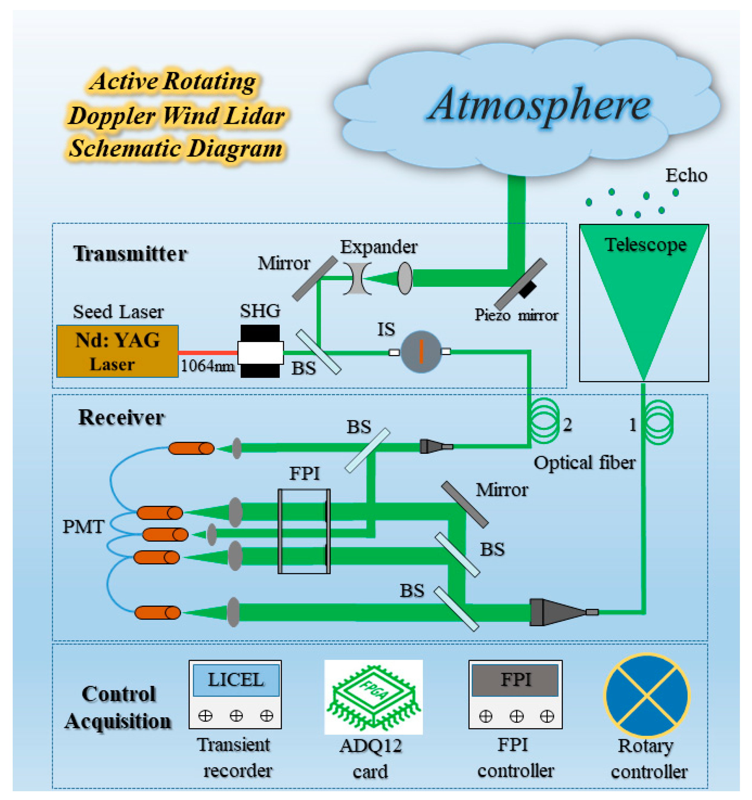
2. Doppler Wind Lidar System

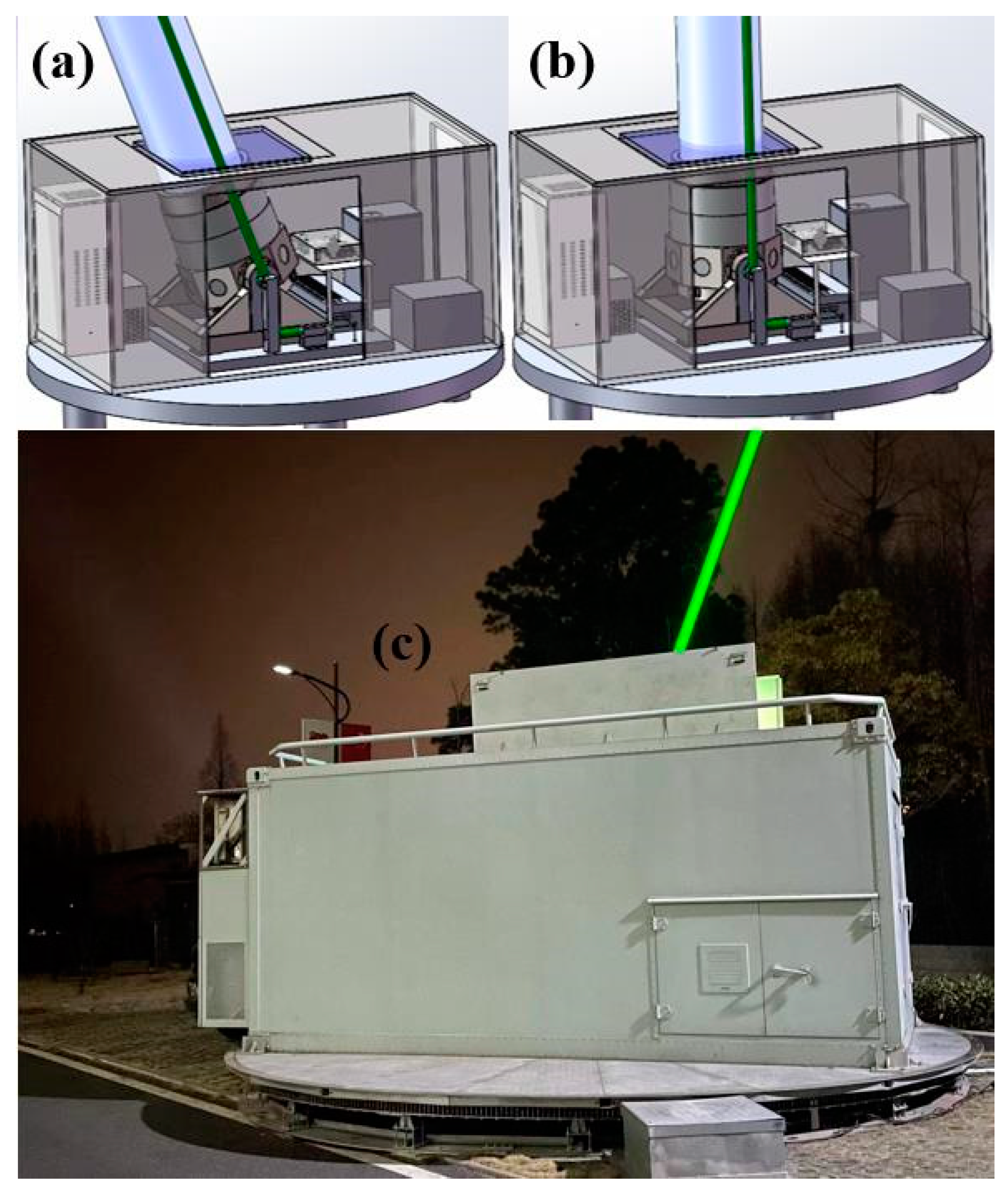
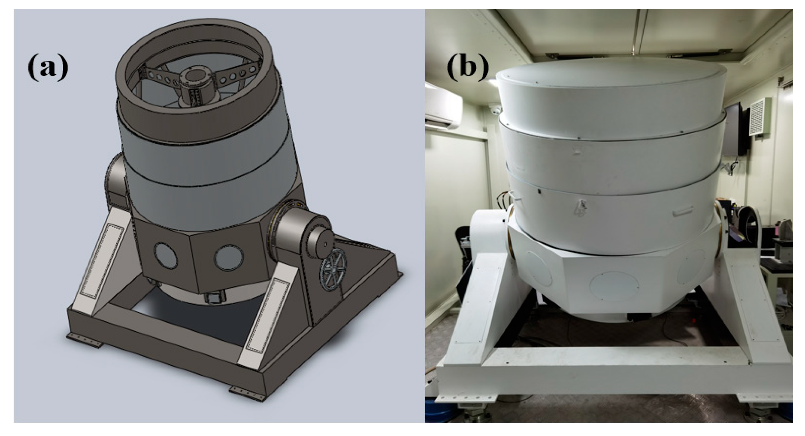
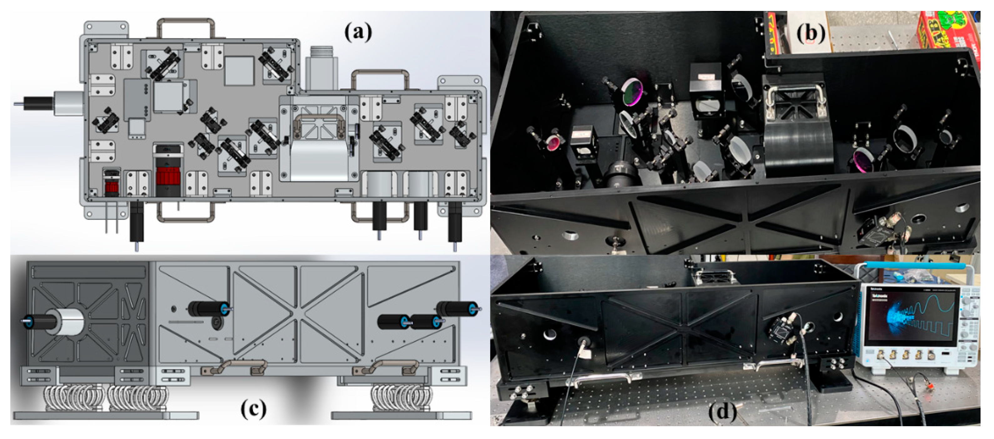
2.1. Whole Structure

Unlike the previous use of multiple wind Lidars to detect atmospheric wind fields, the system is embedded in a 5 m × 2.7 m × 2.4 m mobile equipment cabin. The equipment cabin is placed on a circular turntable with a diameter of 6m, which can realize 360° rotation. As shown in Figure 1, the Doppler wind Lidar can perform vertical and oblique detection, respectively. The overall design of Lidar is shown in Figure 2, which mainly includes three subsystems: laser transmitter, receiver, control, and acquisition.

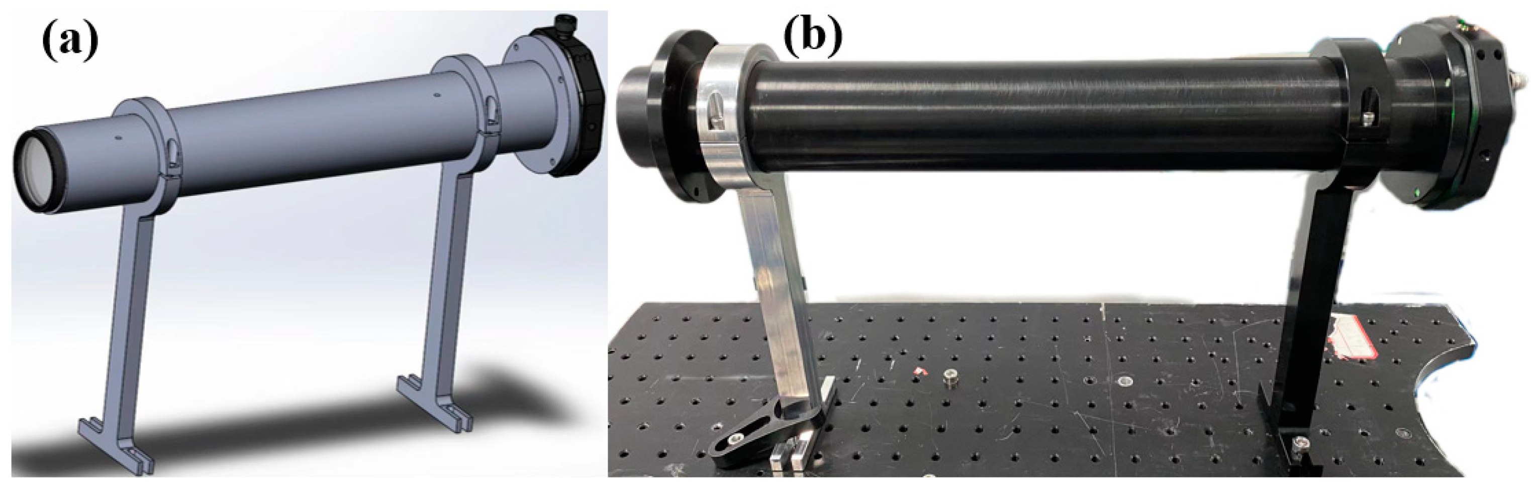
2.2. Transmitter System

A Q-switched Nd: YAG laser (Powerlite 9030, Continuum Ltd., Winchester, UK) with an operating wavelength of 532 nm, an output energy of about 350 mJ/pulse, and a repetition rate of 30 Hz was used. The transmission divergence angle is reduced to around 50 μrad when the laser beam is magnified by a factor of 10. This decreases the telescope’s field of vision. During Lidar detection, an Integrating sphere (IS), an optical fiber, and a collimator were used to homogenize 1% of the emitted light before sending it to the receiver for Fabry-Perot interferometer frequency locking (FPI). The transmitter’s precise specifications are shown in Table 1.

2.3. Receiver System

A Cassegrain telescope with a diameter of 800 mm and a focal length of 1961 mm was used to collect the echo signals. A 200 μm core diameter fiber was used to transmit the signal light from the telescope to the receiver. Therefore, the FOV of the telescope is limited to 100 μrad. The other end of the fiber is fixed on a collimator with a divergence angle of 2.5 mrad. A 0.3 nm FWHM narrowband interference filter for background suppression was mounted on both collimators. Five photomultiplier tubes (PMTs) were used in the receiver as shown in Figure 2. PMT 1 detects 10% of the atmospheric echo signal as the assessment benchmark for the transceiver system’s alignment. PMTs 2 and 3 detect leftover beams entering the two edge channels of the FPI in order to determine Doppler shift. In addition, they are gated by an electrical strobe card with a delay of 80 milliseconds to prevent signal saturation at low altitudes. The transmittance of the frequency-locked FPI channel is detected using PMTs 4 and 5. Table 2 lists the exact specifications of the receiver.
The FPI with an optical aperture of 80 mm and an operating wavelength of 532 nm is the key device for Doppler shift identification. It consists of two 38 mm diameter edge channels and a 19 mm diameter frequency locked channel. The spectrum follows a Lorentz curve and the spectral bandwidth and spacing between the two edge channels has a significant effect on the signal-to-noise ratio (SNR) and the sensitivity of frequency discrimination of the two channels. Additionally, the presence of the Mie scattering component in the lidar echo can cause errors in wind speed measurements due to its much narrower spectrum compared to Rayleigh-Brilliance scattering. In general, separate treatment of the Mie scattering signal and the Rayleigh scattering signal is required. It is also possible to choose a location with similar sensitivity of the two scattering signals during the measurement, thus effectively reducing the effect of aerosols. Taking the aerosol backscattering coefficient of 1.5, the temperature of 230 K, the height of 20 km, and the wind speed size of 20 m/s, the effect of meter scattering and Rayleigh scattering on the wind speed error is shown in Figure 3. It can be seen that the position of the red line is the position where the minimum wind speed error is affected by the Mie scattering and Rayleigh scattering, and the linear fitted line is y = 0.701975x + 2.696085. When the FWHM is 1.05 GHz, the bimodal spacing is 3.48 GHz, and the wind speed error is less than 3 m/s. Combining the above two points and the design index of the system, when the working wavelength is 532 nm and the wind speed measurement range is ±100 m/s, the free spectral spacing of FPI is determined to be 8.51 GHz, the bandwidth is 1.05 GHz, the effective fineness is 7.09, and the spacing between the two edge channels is 3.48 GHz.
After determining the parameters of the FPI, the other parameters of the receiver are calculated. The wind speed error at different heights was analyzed for the effect of different divergence angles on the wind measurement accuracy. As shown in Figure 4, according to the sensitivity and the corresponding frequency response function, with the signal-to-noise ratio equal to 50, it can be seen that the wind speed at low and high levels is more obviously affected by the divergence angle, and the radial error increases gradually with the increase in the divergence angle, especially when the divergence angle is greater than 3 mrad, the radial wind speed error increases rapidly.
In summary, if the divergence angle of the receiver is 5 mrad, the sensitivity will be reduced by 15%, which will widen the transmittance curve of the locking channel away from the half height, affecting the frequency locking performance of FPI and reducing the accuracy of wind measurement. Considering the compactness and adjustability of the receiver size and internal structure, the divergence angle should be set within 3 mrad. The use of fiber with a core diameter of 0.22 and a spot diameter of 30 mm can effectively reduce the design difficulty of beam splitter and reflector.

2.4. Control and Acquisition System

An industrial control computer was used to control the overall Doppler wind laser system. The dynamic range of the atmospheric Rayleigh scattering signal from 10 to 50 km is about five orders of magnitude, and the long-distance signal strength is in the order of uV. Therefore, a high dynamic range transient recorder (TR20-160, Licel GmbH, Berlin, Germany) and a high-speed acquisition card (ADQ12, Queentest Ltd., Hongkong, China) were used for data acquisition, respectively. For strong low-altitude signals, the transient recorder uses an AD analog-to-digital conversion module with a sampling accuracy of 12 bits to collect uA-level data. The transient recorder employs a PC photon counting module with a sampling precision of 250 MHz to gather data at the level of single photons for weak signals at high altitudes. Thus, the AD and PC profiles have been glued together to improve the dynamic range of detection. Specifically, the AD signal profile is shifted forward by 9 bins to correct for its electronic delay relative to the PC channel. Additionally, the pileup effect is corrected for PC signals before the implementation of the gluing process. In general, the photon counter is a non-paralyzable system, the real photon counting rate can be calculated from the measured values:
P = P / 1 τ · P ,
where P’ is the real photon counting rate, P is the measured photon counting rate, and τ is the dead time, about 4 ns. The segments with a PC amplitude from 2 to 4 MHz were chosen for merging. Next, the combined portion of the AD and PC signals are weighted:
P G   = 1 W · P A D   + W · P p c   ,
W = 0 ,     P p c   i m i n ( P p c   i m i n ) / i m a x i m i n ,   i m i n P p c   i m a x   , 1 ,   P p c   i m a x
where P G   is the spliced signal, P A D   and P p c   are the calculated fitting polynomials, W is the fusion coefficient, i is the fusion interval and i m i n , i m a x are the maximum and minimum values. For example, the results of signal gluing for the Edge 1 channel are illustrated in Figure 5.
After integrating the two modalities, the dynamic detection range may approach 6–8 orders of magnitude. The specific parameters of the control and acquisition system are shown in Table 3.

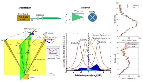
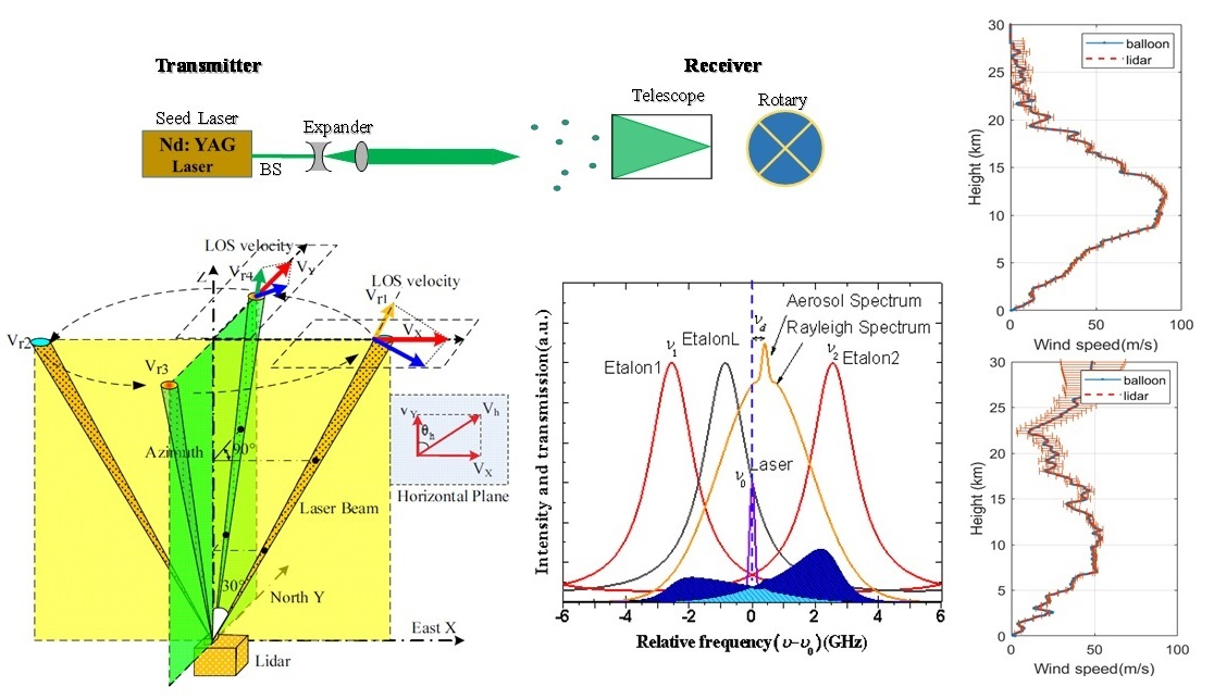
2.5. Inversion Principle for Wind Speed

The double-edge technology inherits the advantages of the single-edge technology. The light passing through the edge filter will interfere several times, making the transmission rate and light intensity of the backward scattered light change. The Doppler shift information it carries is calculated to obtain the frequency response function and ultimately the inversion to obtain the change in wind speed. The lidar designed in this manuscript measures the velocities of sight (VOS) in each of the four directions in turn. The vertical wind speed is assumed to be zero and the horizontal wind field is synthesized by vectoring. Specifically, this can be expressed by the following equation:
V   = V X   + V Y   ,
V X   = ( V dE V dW ) / 2 sin θ ,
V Y   = ( V dN V dS ) / 2 sin θ ,
d = arctan V X   V Y + π 1 sin ( V Y   + V Y ) · V X   ,
where V and d are the horizontal wind speed and direction, respectively. V X   and V Y   are the vector components of the horizontal wind speed, respectively. V dE , V dW , V dS , V dN are the east, west, south and north VOSs, respectively, and θ is the zenith angle.

3. Performance Studies of Transmitter and Receiver

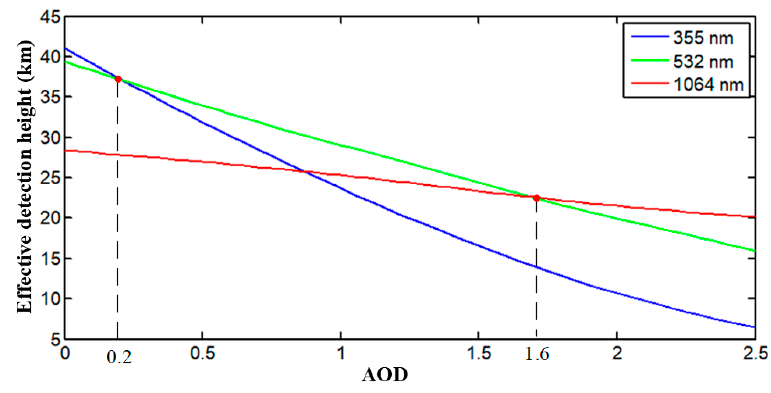
3.1. Laser Wavelength Selection

According to the Lidar equation of Formula (8), the main atmospheric factors affecting the echo signal strength are the backscattering coefficients of molecules and aerosols at different heights, and the atmospheric transmittance between the Lidar and the height to be measured [24,25]:
P z = E 0 c T A r β z z 2 e x p 2 z 0 z α z d z ,
where P z epresents the echo signal intensity detected by the Lidar at a distance z , E 0 is the single pulse energy of the Lidar, c is the speed of light, T is the total transmittance of the Lidar system, A r is the effective receiving area of the telescope, z 0 is the initial height,   α z ,   β z are the extinction coefficient and backscattering coefficient at the distance z , respectively. According to the US Standard Atmosphere Model (USSA-76), the Rayleigh scattered light intensity is inversely proportional to the incident wavelength λ4, and the aerosol backscattering coefficient is inversely proportional to λ1.3. Based on the actual system parameters combined with the atmospheric molecular backscattering coefficient, atmospheric aerosol backscattering coefficient and atmospheric transmittance, the effective detection heights of the three wavelengths under different optical thickness (AOD) conditions are simulated and calculated. As shown in Figure 6, the effective detection height of 355 nm is the highest on clean days when the AOD is less than 0.2, and the effective detection height of 1064 nm is the highest on heavily polluted days when the AOD is greater than 1.6. For optical thicknesses greater than 0.2 and less than 1.6, 532 nm has the highest effective detection height. It is not difficult to explain that the effect of the atmosphere on the SNR of a signal at a given detection height is determined by both the scattering term and the transmittance. In terms of the scattering term, shortwave is more advantageous, but accordingly, the attenuation of the shortwave signal by pollution is also more severe. Taking the above together, it can be assumed that 532 nm is the most suitable wavelength for obtaining all-weather stratospheric atmospheric wind field information for a long period of time.

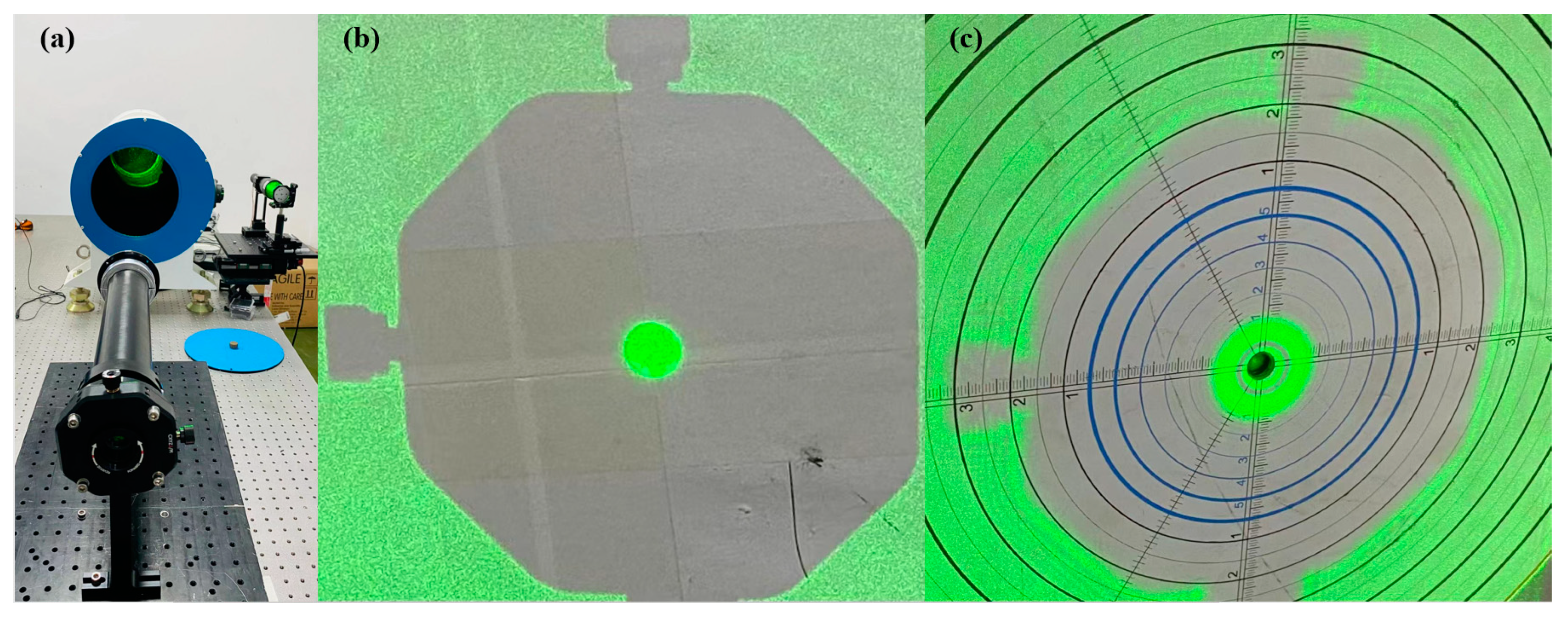
3.2. Laser Beam Expander Optimization

It can be seen from the above that when the atmospheric echo light is coupled into the receiver by the optical fiber and transmitted to the FPI, the divergence angle will inevitably appear in the process. The frequency corresponding to the peak FPI transmittance at ideal positive incidence of the beam with no divergence angle is used as a reference (frequency 0). The effect of different incident light divergence angles on the transmittance curve, velocity sensitivity and wind speed measurement error are explicitly shown in Figure 5. It can be seen from Figure 7a that with the increase in the beam divergence angle, not only the spectrum of the transmittance curve is broadened, but also the peak transmittance decreases. Figure 7b illustrates the sharp drop in velocity sensitivity when the divergence angle exceeds 2.5 mrad at zero Doppler shift. Figure 7c shows the variation of wind speed measurement error with divergence angle. When the divergence angle increases from 2 mrad to 3 mrad, the systematic measurement error increases from 6.1% to 6.28%. When the emission angle increases from 3 mrad to 3.5 mrad, the system measurement error increases to 13.6%, so the beam divergence angle of this system should be controlled within 3 mrad. At the same time, according to the relationship between the full angle of FPI divergence and the coupling fiber [26,27]:
2 θ 0 d e 2 arcsin ( N . A . ) d f ,
where 2θ0 is the etalon divergence full angle, N.A. = 0.22 is the numerical aperture of the fiber, df = 200 μm is the core diameter of the fiber, and de = 38 μm is the etalon diameter. Finally, the divergence angle of the FPI of this system is about 2.5 mrad.
Given that the focal length of the Cassegrain telescope is 1961 mm and the focal length of the collimator is 80 mm, the system’s receiving field of vision is 0.1 mrad. In order to enable the telescope to receive all the signals, the divergence angle of the outgoing laser should be controlled to be less than 0.2 mrad, and it is optimal to be within half of the receiving field of view. Since the divergence angle of the emitted laser is 0.5 mrad, a ten-fold beam expander is designed to compress the divergence angle of the emitted laser to 0.05 mrad. Considering that the focus of the Kepler-type beam expander is located between the objective lens and the imaging lens, the laser energy will be focused and the air temperature between the lenses will increase, resulting in wavefront errors. Because of this, the system beam expander is finally designed as a Galilean-style structure consisting of a spherical mirror and an aspherical mirror. Combined with ZEMAX software, the initial structure of the beam expander is simulated and optimized. The optimized structure parameters are shown in Table 4, and the emission optical path is shown in Figure 8.
Tolerance analysis of the beam expander is a crucial step after the optical system design and manufacturing of optical parts. Scientific and practical tolerance analysis is very important for the adjustment of the optical system, which improves the efficiency and accuracy of the adjustment. Therefore, the beam expander’s element tolerance and surface tolerance were analyzed using the Monte Carlo method in ZEMAX. In laser beam expander mounting, the primary mirror is installed first as a reference and then the secondary mirror is installed for overall mounting. In this process, the main tolerances to be analyzed are: the radius tolerance and secondary term coefficient tolerance of the primary mirror; the radius tolerance and secondary term coefficient tolerance of the secondary mirror; the relative eccentric tilt tolerance between the two mirrors and the mirror spacing tolerance. In ZEMAX, given a moderate amount of machining error, a series of random lenses are generated. Combined with the system wavefront root mean square (RMS) of the beam expander in Figure 9, 5000 Monte Carlo experiments were carried out, and the sampling results in Table 5 were obtained. It can be seen that the RMS of 90% of the sampled wavefronts is less than 0.0783, which is less than 1/12λ to meet the wave aberration RMS requirements of the laser beam expander emission system. It should be emphasized that the radius of curvature of the primary and secondary mirrors has a large impact on the system and needs to be strictly controlled. In addition, as the general optical system requires operation at 20 °C and one standard atmosphere, air conditioning and circulation fans are used in the equipment cube.
After meeting the tolerance requirements, the optimized laser beam expander was designed and manufactured, as shown in Figure 10. The actual divergence angle of the beam expander needs to be confirmed by a test before it is formally put into the Doppler wind measurement experiment. To avoid the influence of temperature and other environmental factors, the experiment chose to test the beam expander in a constant-temperature optical laboratory using a parallel light tube and a laser at 532 nm. It is known that the divergence angle of the parallel light tube is 0.09 mrad. By comparing the near-field spot with the spot after 23 m light range, the result shows that the spot changes from 10 mm to 30.2 mm at the time of emission, which meets the standard of beam expansion to meet the design requirements, as shown in Figure 11.

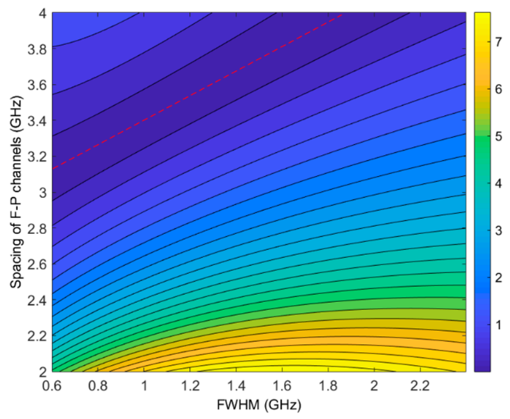
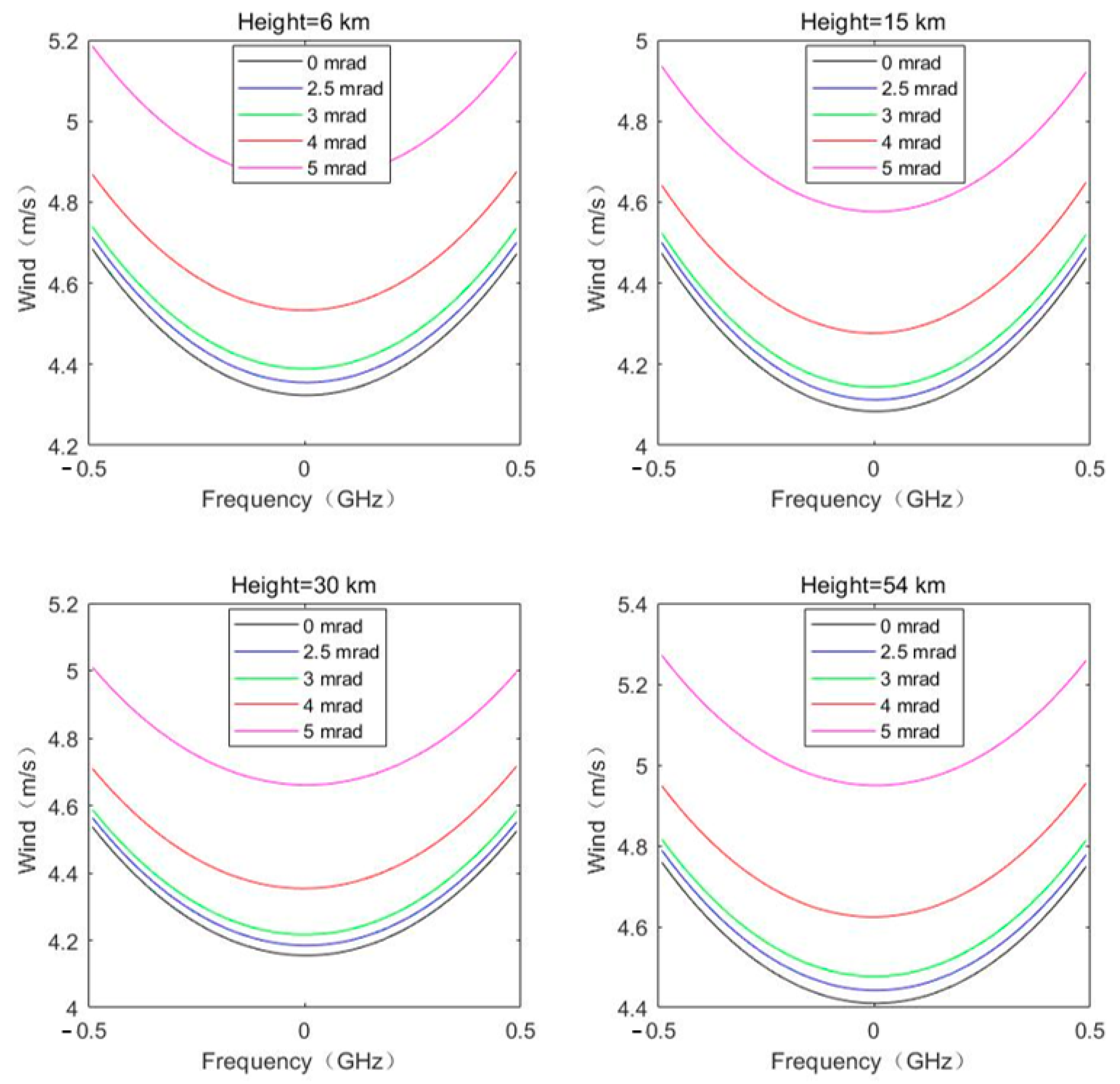
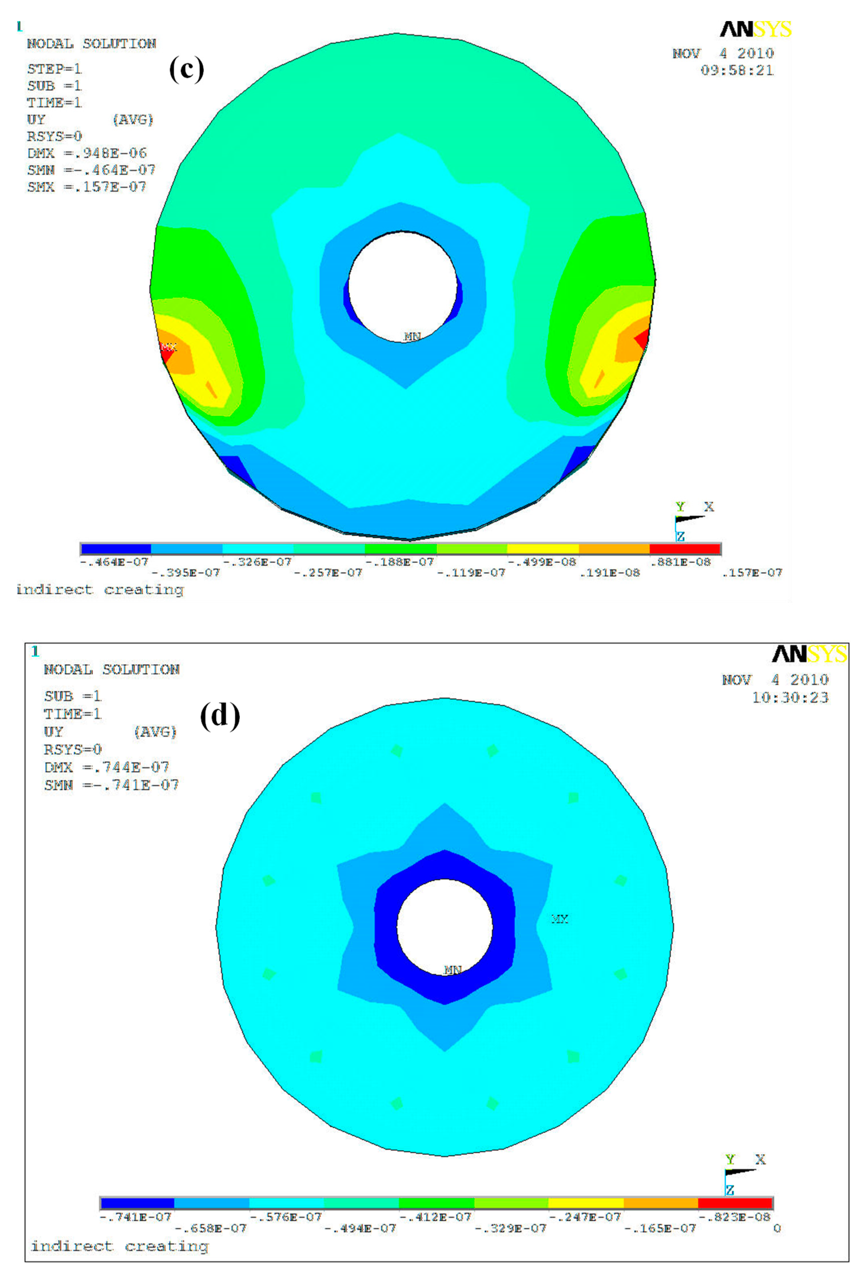
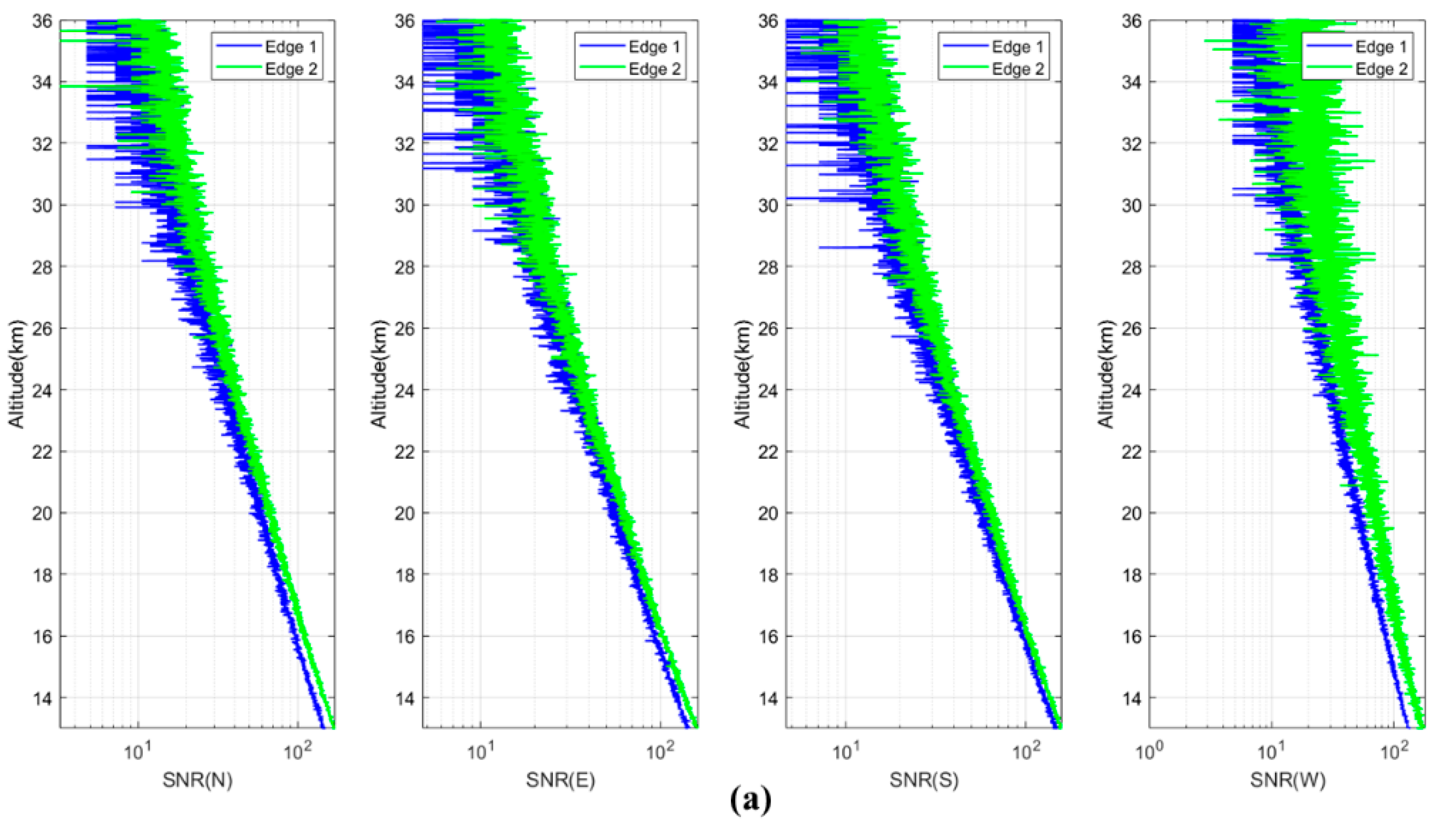
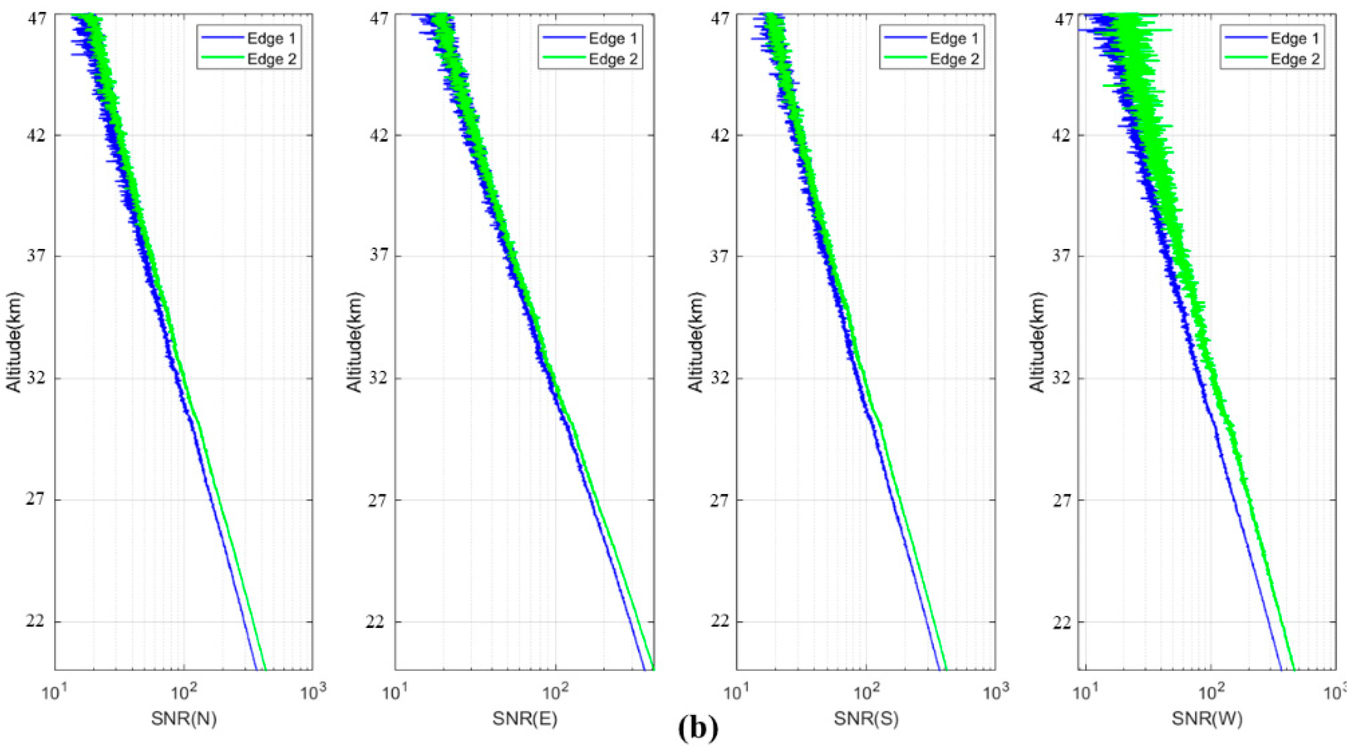
3.3. Receiver Optimization

Because the system uses a Cassegrain telescope with an aperture of 800 mm, the stability of the structure is affected by rotation, so the materials and structure were upgraded. The main part of the mirror barrel is rolled and welded with thin steel plate, and the stiffness and stability of the structure was improved. The main mirror adopts the bottom support structure commonly used in optical inspection, plus a number of auxiliary side supports. The secondary mirror can be adjusted in five dimensions. A set of correction mirrors are added in front of the focal point to expand the field of view and correct the aberration. Each mirror chamber is installed in the corresponding mirror barrel structure with a beautiful appearance. The base of the telescope has four connection plates welded to the bottom of the base, with holes spaced 50 mm apart, for threaded connection to the optical platform. In addition, the base is designed with two leveling gauges with an accuracy of 0.05°/1000 mm, designed to guarantee an accuracy of better than 2° during the levelling process. Pitch axis rotation adopts a manual rocker method, through a set of worm gear and a set of gear two-stage deceleration, which can realize continuous rotation in the range of −10~40°. The resolution of the pitch adjustment dial is 0.5°, and the vernier type pointer is used, while the pitch rotation has a locking function. The mirror chamber can keep the main mirror stable during the scanning process and protect the main mirror safely during transportation. The mirror chamber keeps the main mirror stable during the scanning process and protects it during transport in the vehicle. For this reason, its interior is of welded construction with fixed supports to position the mirror radially and axially, respectively. The bottom center hole is provided with a water connection for the main mirror to be cleaned. The telescope adopts an eighteen point fixed support at the bottom of the main mirror, radial support at three places around the lens, and a classical support method for the auxiliary compression mirror. To verify the reliability of this support method, the finite element software ANSYS was used to model and analyze the main mirror, and the results are shown in Table 6 and Figure 12. It can be seen that the accuracy of the face shape of the main mirror can meet the system design requirements under both operating conditions. The upgraded 800 mm Cassegrain telescope is shown in Figure 13.
The structural stability of the receiver is directly related to the quality of the acquired signal, so further optimization of the receiver structure is needed, as shown in Figure 14. The entire receiver is placed inside a chassis with dimensions of 600 mm × 550 mm × 300 mm. The fiber optic interface is set outside the chassis to facilitate optic-fiber plugging and unplugging. To improve the stability of the receiving optical path, all optical lenses in the receiver use a one-dimensional adjustment mechanism, which makes it easy to adjust the optical path. The detector is placed on the outside of the chassis, which not only reduces the receiver’s size and facilitates the detector’s replacement, but also improves the overall structure of light shielding. In addition, two spring-loaded rope dampers were installed at the bottom of the receiver to prevent high-frequency vibrations caused by the rotation of the platform during the detection experiment.
Figure 14 and the previous introduction show that a total of five PMTs were installed in the receiver to achieve highly sensitive detection in the 532 nm visible band. In order to cooperate with the transient recorder to collect the optimal signal, a single-channel atmospheric echo test was conducted to compare different models of PMTs, and the test results are shown in Table 7. After considering the signal amplitude (MHz), background noise, electromagnetic interference and detection height at SNR = 3, the PMT with serial number AAA0545 (Gate) and model number R7400-02 was selected. The measurement spectrum of this PMT is in the 300–650 nm band with a peak wavelength of 420 nm, quantum efficiency of more than 50%, and time response of 0.78 ns.

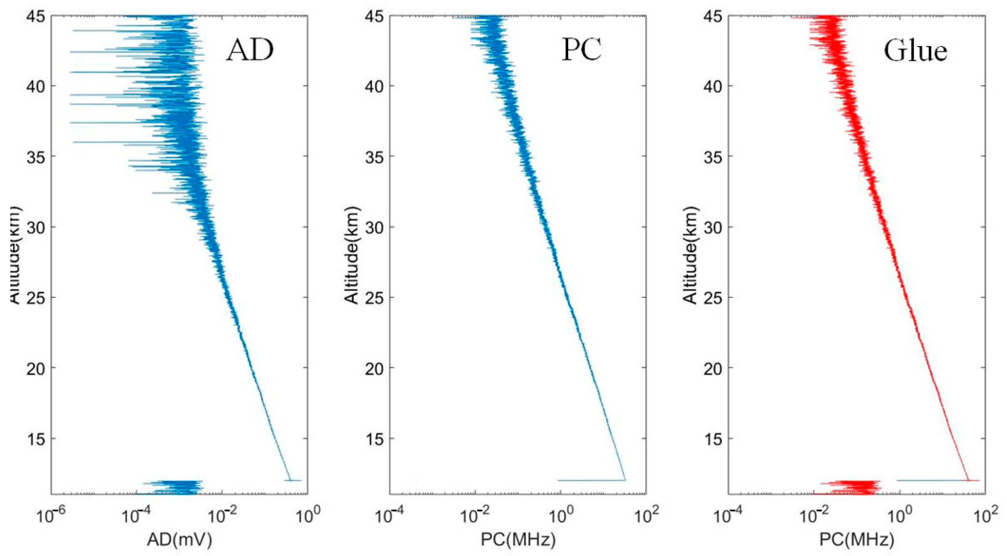
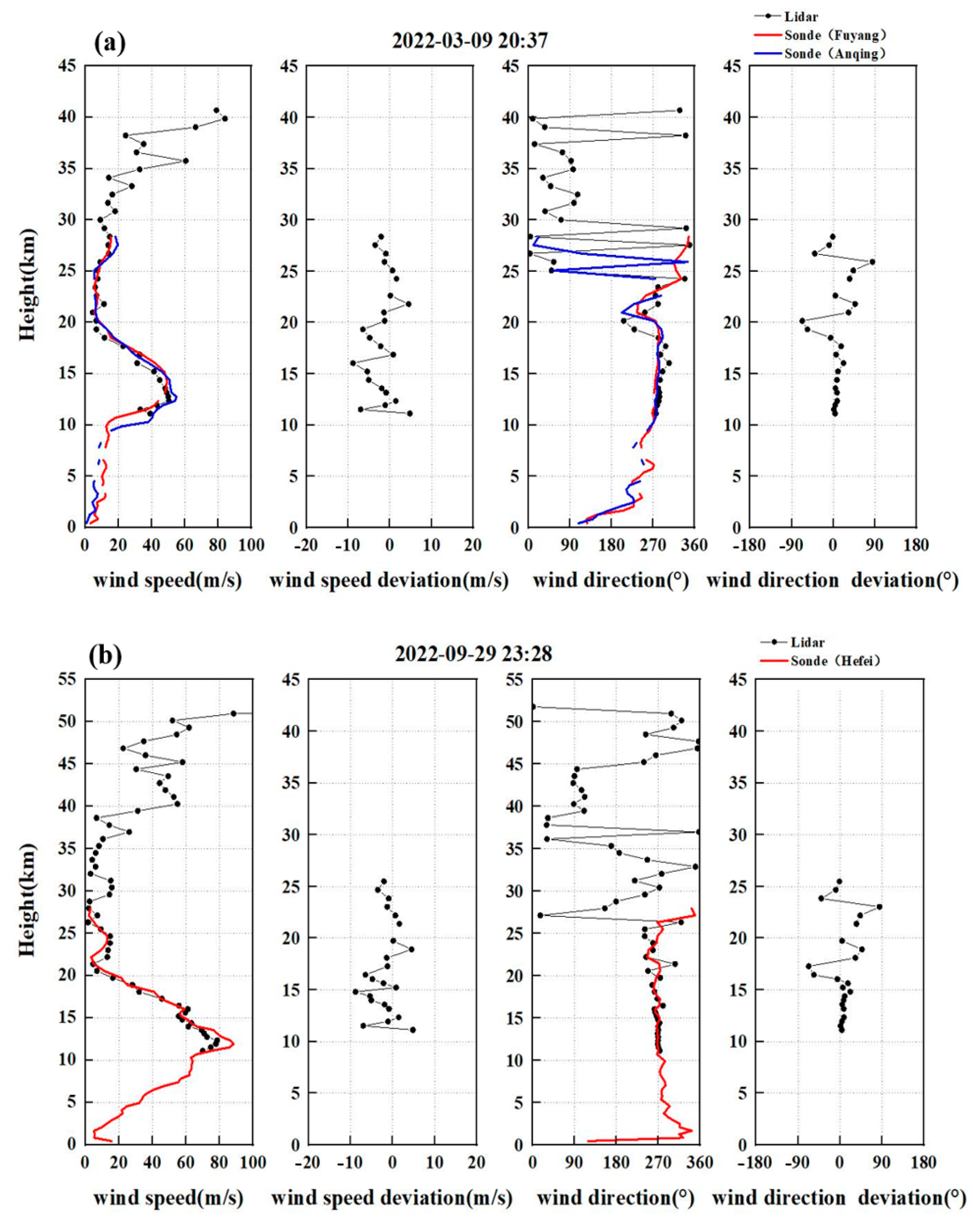
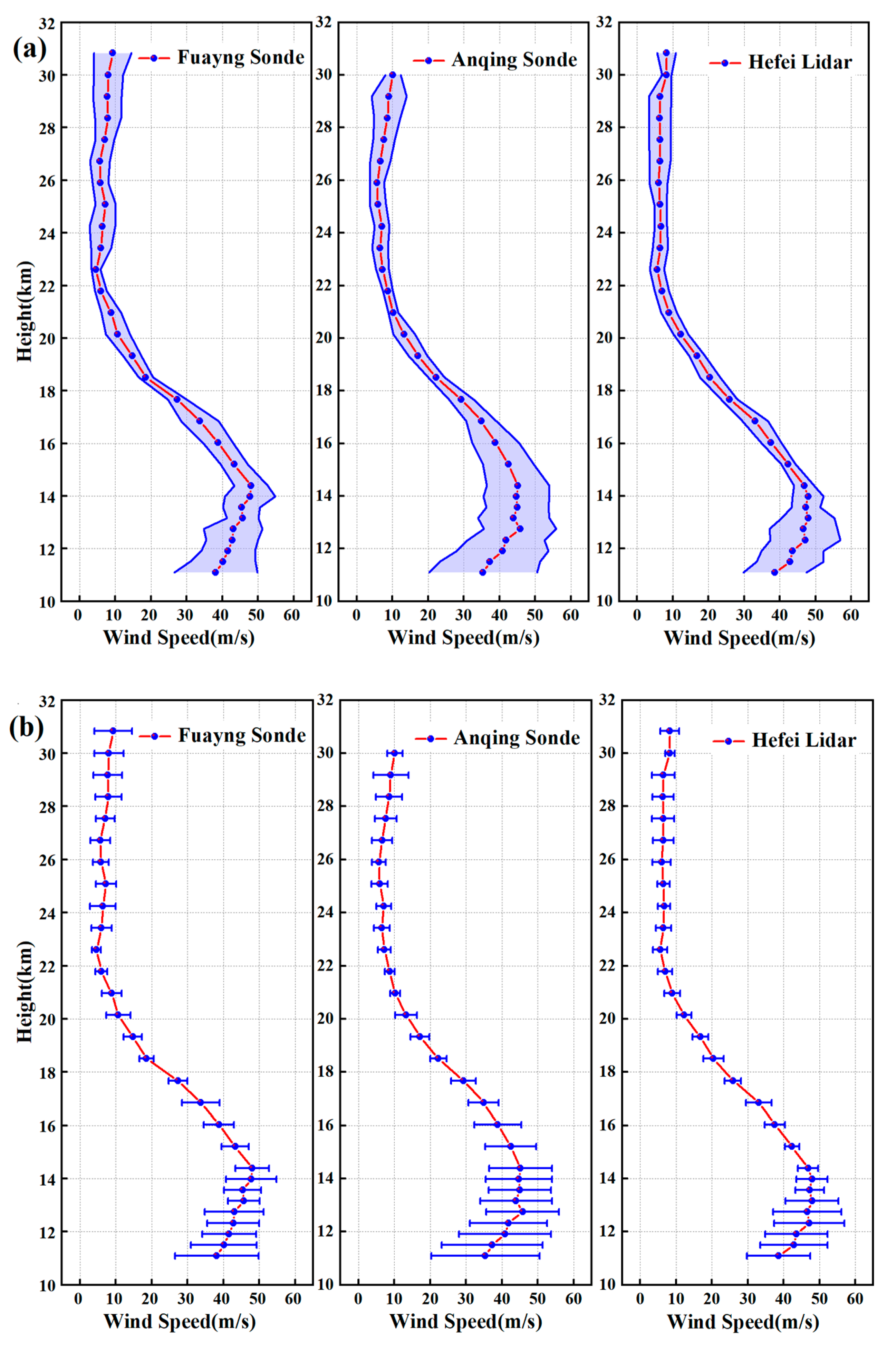
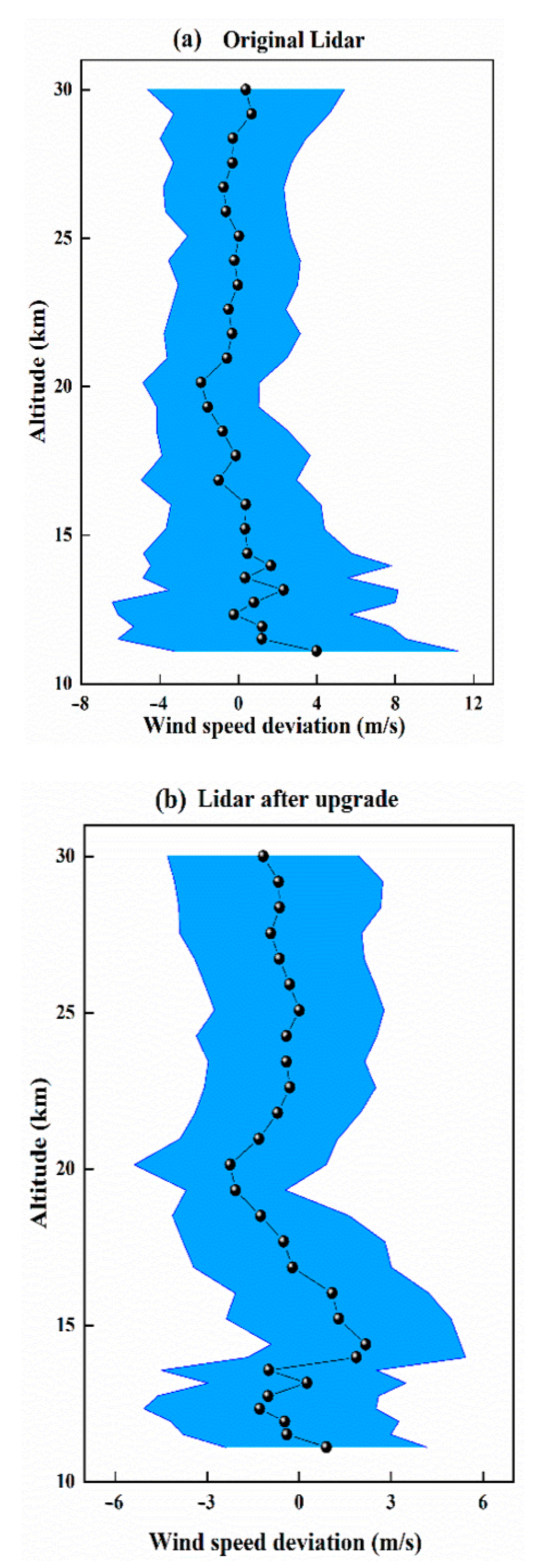
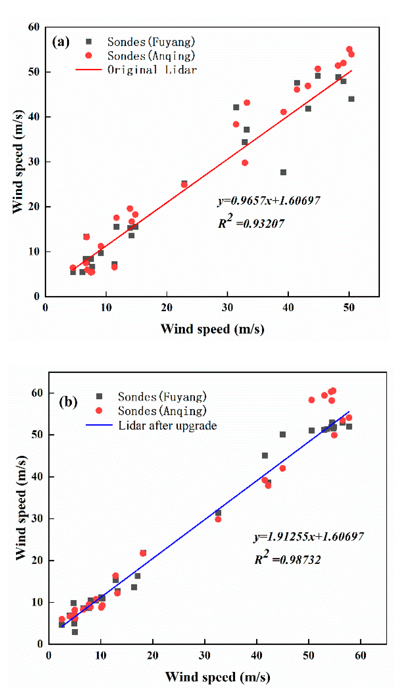
4. Comparison of Detection Results

To validate the impact of transmitter and receiver performance on the system’s ability to detect atmospheric wind fields, Figure 15 and Figure 16 display the experimental findings of the original system and the upgraded system’s capacity to detect atmospheric wind fields. The wind fields detected by Doppler wind Lidar and radiosondes in Anqing and Fuyang areas were compared on 9 March 2022, at around 20:00 (LT). On 29 September 2022, at around 23:00 (LT), the wind fields detected by Doppler wind Lidar and radiosondes in the Hefei area were compared. The raw data were spatially averaged to reach a distance resolution of 300 m to improve the signal-to-noise ratio. To maintain consistency between the two Doppler wind Lidar detection procedures, 8000 laser pulses were fired in each radial direction over the course of 24 min. The Lidar detection profile became effective from 11 km due to an 80-μs delay in gating after the Q switch was turned on. The sounding balloon was launched at the same time and place as the Lidar, and it reached an altitude of about 28 km in 69 min, spanning the duration of the Lidar’s operation. In Figure 15, the SNRs of the four radial directions in the two detection experiments are shown, respectively. Figure 16 then shows the wind speed deviation and wind direction deviation between Lidar and radiosondes. It can be seen that in both detection experiments, the wind speed and direction profiles obtained by Lidar below 30 km (the maximum height of radiosondes) are more similar to the profile trends obtained by radiosondes. However, it is worth noting that without the improved receiver and transmitter, the effective detection altitude of Lidar is only about 36 km. In contrast, the effective detection altitude of the upgraded Lidar is close to 50 km (about 47 km).
To verify the detection stability of this Lidar system after the upgrade, the 36 wind field profiles obtained from October 23 to November 9 were selected for comparison with radiosondes from Anqing and Fuyang. Figure 17 shows the wind field data detected by radiosondes in Fuyang and Anqing and the upgraded Lidar located in Hefei, respectively.
To verify the detection accuracy of the upgraded Lidar, the wind speed profiles detected by Lidar before and after the upgrade were further compared with radiosondes for analysis. It can be seen from Figure 18 that the deviation of wind speed between the upgraded Lidar and radiosondes is significantly smaller than that of the original Lidar. and it can also be found from Figure 19 that the correlation coefficient R2 of the data detected by the upgraded Lidar and radiosondes is 0.98732, which is significantly higher than that of the original Lidar at 0.93207. Combining the above results, it is easy to find that the detection height and accuracy of the designed Doppler wind lidar system are extremely dependent on the performance of the transmitter and receiver. After optimizing and upgrading the beam expander, receiver structure and PMT, the proposed active rotating tropospheric stratospheric Doppler Lidar reaches a detection height of 47 km and the horizontal wind speed deviation is less than 6 m/s. It is worth proposing that the detection accuracy by Lidar at 11–30 km (the average maximum height of radiosondes) is higher than that of radiosondes because it can achieve continuous observation.

5. Conclusions

In summary, this manuscript specifically analyzes the effects of transmitter and receiver on the detection performance of an active rotating tropospheric stratospheric Doppler wind Lidar. First, a 532 nm laser with a good balance of transmission and scattering suitable for all-weathers was chosen as the detection wavelength. After ZEMAX simulation optimization and laboratory setup, a Galilean ten-fold beam expander composed of a spherical mirror and an aspherical mirror was built to reduce the outgoing laser divergence angle to 0.05 mrad. Upgrades were also made to the support methods and structural materials of the 800 mm Cassegrain telescope. On the other hand, the receiver structure has been optimized and reduced in size to facilitate detector replacement, which not only facilitates optical path adjustment but also improves the stability of the received optical path. The best-performing PMT was selected by single-channel atmospheric echo signal testing. Finally, the results of atmospheric wind fields detected by Lidar with upgraded receivers and transmitters were compared with the original Lidar and radiosondes. The results show that the upgraded Lidar can effectively detect the atmospheric wind field at an altitude of about 47 km, and the wind speed deviation is less than 6 m/s. Moreover, the wind speed and wind direction profiles are more consistent with the radiosondes data. Future applications of the proposed active rotating Doppler wind Lidar system will include detection of tropospheric and stratospheric wind fields in various areas and seasons.

Author Contributions

Supervision, conceptualization, funding acquisition, C.X.; methodology, resources, K.X.; software, B.W.; data curation, J.J.; writing—original draft preparation, J.C.; writing—review and editing, M.Z. All authors have read and agreed to the published version of the manuscript.

Funding

This work was supported in part by the Strategic Priority Research Program of the Chinese Academy of Sciences (XDA17040524), Anhui Province 2017 High-level Science and Technology Talent Team Project (010567900), Key Program of 13th Five-Year Plan, CASHIPS (KP-2019-05) and Civil Aerospace Technology Pre-research Project (D040103).

Data Availability Statement

The data presented in this study are available on request from the corresponding author.

Acknowledgments

The authors thank Xie Chenbo of Anhui Institute of Optics and Fine Mechanics, Hefei Institutes of Physical Science, Chinese Academy of Sciences for providing the data.

Conflicts of Interest

The authors declare no conflict of interest.

Correction Statement

This article has been republished with a minor correction to the existing affiliation information. This change does not affect the scientific content of the article.

References

  1. Solovjova, T.; Makarov, N.; Rees, D.; Fahrutdinova, A.; Guryanov, V.; Fedorov, D.; Korotyshkin, D.; Forbes, J.; Pogoreltsev, A.; Kurschner, D.M. Semi-empirical model of middle atmosphere wind from the ground to the lower thermosphere. Adv. Space Res. Off. J. Comm. Space Res. (COSPAR) 2009, 43, 239–246. [Google Scholar]
  2. Yang, J.; Xiao, C.; Hu, X.; Xu, Q. Responses of zonal wind at ~40°N to stratospheric sudden warming events in the stratosphere, mesosphere and lower thermosphere. Sci. China Technol. Sci. 2017, 60, 935–945. [Google Scholar] [CrossRef]
  3. Wang, Z.; Liu, Z.; Liu, L.; Wu, S.; Liu, B.; Li, Z.; Chu, X. Iodine-filter-based mobile Doppler lidar to make continuous and full-azimuth-scanned wind measurements: Data acquisition and analysis system, data retrieval methods, and error analysis. Appl. Opt. 2010, 49, 6960–6978. [Google Scholar]
  4. Hedin, A.; Fleming, E.; Manson, A.; Schmidlin, F.; Avery, S.; Clark, R.; Franke, S.; Fraser, G.; Tsuda, T.; Vial, F.; et al. Empirical wind model for the upper, middle and lower atmosphere. J. Atmospheric Terr. Phys. 1996, 58, 1421–1447. [Google Scholar] [CrossRef]
  5. Dou, X.; Han, Y.; Sun, D.; Xia, H.; Shu, Z.; Zhao, R.; Shangguan, M.; Guo, J. Mobile Rayleigh Doppler lidar for wind and temperature measurements in the stratosphere and lower mesosphere. Opt. Express 2014, 22, A1203–A1221. [Google Scholar] [CrossRef]
  6. Hao, R.; Dou, X.; Xue, X.; Sun, D.; Han, Y.; Chen, C.; Zheng, J.; Li, Z.; Zhou, A.; Han, Y.; et al. Stratosphere and lower mesosphere wind observation and gravity wave activities of the wind field in China using a mobile Rayleigh Doppler lidar. J. Geophys. Res. Space Phys. 2017, 122, 8847–8857. [Google Scholar]
  7. Gentry, B.M.; Chen, H.; Li, S.X. Wind measurements with 355-nm molecular Doppler lidar. Opt. Lett. 2000, 25, 1231–1233. [Google Scholar] [CrossRef]
  8. Feifei, L.; Decang, B.; Heng, L.; Lucheng, Y.; Mingjian, W.; Xiaopeng, Z.; Jiqiao, L.; Weibiao, C. Principle Prototype and Experimental Progress of Wind Lidar in Near Space. Chin. J. Lasers 2020, 47, 0810003. [Google Scholar] [CrossRef]
  9. Souprayen, C.; Garnier, A.; Hertzog, A. Rayleigh-Mie Doppler wind lidar for atmospheric measurements. II. Mie scattering effect, theory, and calibration. Appl. Opt. 1999, 38, 2422–2431. [Google Scholar]
  10. Ansmann, A.; Wandinger, U.; Le Rille, O.; Lajas, D.; Straume, A.G. Particle backscatter and extinction profiling with the spaceborne high-spectral-resolution Doppler lidar ALADIN: Methodology and simulations. Appl. Opt. 2007, 46, 6606–6622. [Google Scholar] [CrossRef]
  11. Baumgarten, G. Doppler Rayleigh/Mie/Raman lidar for wind and temperature measurements in the middle atmosphere up to 80 km. Atmospheric Meas. Tech. 2010, 3, 1509–1518. [Google Scholar] [CrossRef]
  12. Huffaker, R.M.; Reveley, P.A. Solid-state coherent laser radar wind field measurement systems. Pure Appl. Opt. J. Eur. Opt. Soc. Part A 1998, 7, 863–873. [Google Scholar]
  13. Zhao, Y.; Zhang, X.; Zhang, Y.; Ding, J.; Wang, K.; Gao, Y.; Su, R.; Fang, J. Data Processing and Analysis of Eight-Beam Wind Profile Coherent Wind Measurement Lidar. Remote Sens. 2021, 13, 3549. [Google Scholar] [CrossRef]
  14. Zhang, H.; Liu, X.; Wang, Q.; Zhang, J.; He, Z.; Zhang, X.; Li, R.; Zhang, K.; Tang, J.; Wu, S. Low-Level Wind Shear Identification along the Glide Path at BCIA by the Pulsed Coherent Doppler Lidar. Atmosphere 2020, 12, 50. [Google Scholar] [CrossRef]
  15. Guo, W.; Shen, F.; Shi, W.; Liu, M.; Wang, Y.; Zhu, C.; Shen, L.; Wang, B.; Zhuang, P. Data inversion method for dual-frequency Doppler lidar based on Fabry-Perot etalon quad-edge technique. Optik 2018, 159, 31–38. [Google Scholar] [CrossRef]
  16. Shen, F.; Xie, C.; Qiu, C.; Wang, B. Fabry-Perot etalon-based ultraviolet trifrequency high-spectral-resolution lidar for wind, temperature, and aerosol measurements from 0.2 to 35 km altitude. Appl. Opt. 2018, 57, 9328–9340. [Google Scholar] [CrossRef]
  17. Shen, F.; Ji, J.; Xie, C.; Wang, Z.; Wang, B. High-spectral-resolution Mie Doppler lidar based on a two-stage Fabry-Perot etalon for tropospheric wind and aerosol accurate measurement. Appl. Opt. 2019, 58, 2216–2225. [Google Scholar] [CrossRef]
  18. Shen, F.; Wang, B.; Shi, W.; Zhuang, P.; Zhu, C.; Xie, C. Design and performance simulation of 532 nm Rayleigh-Mie Doppler lidar system for 5–50 km wind measurement. Opt. Commun. 2018, 412, 7–13. [Google Scholar] [CrossRef]
  19. Yan, Z.; Hu, X.; Guo, W.; Guo, S.; Cheng, Y.; Gong, J.; Yue, J. Development of a mobile Doppler lidar system for wind and temperature measurements at 30–70 km. J. Quant. Spectrosc. Radiat. Transf. 2017, 188, 52–59. [Google Scholar] [CrossRef]
  20. Zhang, F.; Dou, X.; Sun, D.; Shu, Z.; Xia, H.; Gao, Y.; Hu, D.; Shangguan, M. Analysis on error of laser frequency locking for fiber optical receiver in direct detection wind lidar based on Fabry-Perot interferometer and improvements. Opt. Eng. 2014, 53, 124102. [Google Scholar] [CrossRef]
  21. Han, Y.; Sun, D.-S.; Weng, N.-Q.; Wang, J.-G.; Dou, X.-K.; Zhang, Y.-H.; Guan, J.; Miao, Q.; Chen, X. Lidar observations of wind over Xin Jiang, China: General characteristics and variation. Opt. Rev. 2016, 23, 637–645. [Google Scholar] [CrossRef]
  22. Straume-Lindner, A.G.; Ingmann, P.; Endemann, M. Status of the Doppler Wind Lidar Profiling Mission ADM-Aeolus; European Space Research and Technology Centre (ESA-ESTEC): Noordwijk, The Netherlands, 1999. [Google Scholar]
  23. Zhao, M.; Xie, C.; Wang, B.; Xing, K.; Chen, J.; Fang, Z.; Li, L.; Cheng, L. A Rotary Platform Mounted Doppler Lidar for Wind Measurements in Upper Troposphere and Stratosphere. Remote Sens. 2022, 14, 5556. [Google Scholar] [CrossRef]
  24. Li, S.; Sun, X.; Zhang, R.; Zhang, C. Simulation of Frequency Discrimination and Retrieval of Wind Speed for the Bistatic Doppler Wind Lidar. Optik 2018, 179, 796–803. [Google Scholar] [CrossRef]
  25. Zhang, C.; Sun, X.; Zhang, R.; Zhao, S.; Lu, W.; Liu, Y.; Fan, Z. Impact of solar background radiation on the accuracy of wind observations of spaceborne Doppler wind lidars based on their orbits and optical parameters. Opt. Express 2019, 27, A936–A952. [Google Scholar] [CrossRef]
  26. Zhao, R.-C.; Xia, H.-Y.; Dou, X.-K.; Sun, D.-S.; Han, Y.-L.; Shangguan, M.-J.; Guo, J.; Shu, Z.-F. Correction of temperature influence on the wind retrieval from a mobile Rayleigh Doppler lidar. Chin. Phys. B 2015, 24, 024218. [Google Scholar] [CrossRef]
  27. Tang, L.; Shu, Z.; Dong, J.; Wang, G.; Wang, Y.; Xu, W.; Hu, D.; Chen, T.; Dou, X.; Sun, D.; et al. Mobile Rayleigh Doppler wind lidar based on double-edge technique. Chin. Opt. Lett. 2010, 8, 726–731. [Google Scholar] [CrossRef]
Figure 1. Active Rotating Tropospheric Stratospheric Doppler Wind Lidar. (a) Tilt detection mode. (b) Vertical detection mode. (c) Schematic diagram of detection work.
Remotesensing 15 00952 g001
Figure 2. The overall design of the Doppler wind Lidar.
Remotesensing 15 00952 g002
Figure 3. Plot of wind speed error with bandwidth and bimodal spacing as independent variables (considering Rayleigh scattering and Mie scattering).
Remotesensing 15 00952 g003
Figure 4. Effect of different incident light divergence angles on radial wind speed errors at different heights.
Remotesensing 15 00952 g004
Figure 5. The results of gluing for the AD and PC signal.
Remotesensing 15 00952 g005
Figure 6. Effective detection heights at three wavelengths at different AOD.
Remotesensing 15 00952 g006
Figure 7. The effects of different incident light divergence angles on (a) transmittance curve (b) velocity sensitivity (c) wind speed measurement error.
Remotesensing 15 00952 g007aRemotesensing 15 00952 g007b
Figure 8. The Beam expander emission light path diagram 3D.
Remotesensing 15 00952 g008
Figure 9. Schematic of the system wavefront of the laser beam expander.
Remotesensing 15 00952 g009
Figure 10. Schematic of the Laser beam expander. (a) Design (b) Solid.
Remotesensing 15 00952 g010
Figure 11. (a) Parallel light pipe test system. (b) Near-field spot. (c) Far-field spot.
Remotesensing 15 00952 g011
Figure 12. The main mirror stress cloud and axial surface shape cloud under different working conditions. (a,c) 30° (b,d) 90°.
Remotesensing 15 00952 g012aRemotesensing 15 00952 g012b
Figure 13. The structural of the upgraded 800 mm Cassegrain telescope. (a) Design diagram (b) Solid diagram.
Remotesensing 15 00952 g013
Figure 14. Schematic diagram of the receiver after structure optimization. (a,c) Design sketches (b,d) Solid drawings.
Remotesensing 15 00952 g014
Figure 15. The SNR profiles in four detection directions. (a) Original (b) Upgraded.
Remotesensing 15 00952 g015aRemotesensing 15 00952 g015b
Figure 16. Comparison of Doppler wind Lidar and radio sounding instrument results. (a) Original (b) Upgraded.
Remotesensing 15 00952 g016
Figure 17. Comparison of atmospheric wind field profiles detected by Doppler wind Lidar and radio sounding instruments from October 23 to November 9. (a) Atmospheric wind field changes (b) Error bars.
Remotesensing 15 00952 g017
Figure 18. Wind speed deviation of Lidar from radiosondes. (a) Original (b) Upgraded.
Remotesensing 15 00952 g018
Figure 19. Correlation coefficient R2 of Lidar and radiosondes detection data. (a) Original (b) Upgraded.
Remotesensing 15 00952 g019
Table 1. Transmitter parameters.
Laser wavelength532.1 nm
Pulse energy350 mJ
Repetition rate30 Hz
FWHM70 MHz
Divergence angle50 μrad
Table 2. Receiver parameters.
Telescope diameter800 mm
FOV100 μrad
FWHM0.3 nm
Fiber core diameters200 μrad
Fiber N.A.0.22
Beam divergence2.5 mrad
Table 3. Control and acquisition parameters.
Transient recorder12 bit@AD, 250 MHz@PC
20 MHz sampling rate
Acquisition card12 bit, 1 GHz sampling rate
CPU≥2.0 GHz
RAM≥4 GB
HDD≥500 GB
Table 4. The optimized beam expander structural parameters.
SurfRadius/mmThickness/mmMaterialDiameter (Half)/mmConic
OBJInfinityInfinity-Infinity0
1Infinity50-50
STO−21.2923.5SILICA80
3Infinity400-80
4Infinity10SILICA550
5−209.82750-55−0.524
IMAInfinity--50.0980
Table 5. Monte Carlo analysis results of the laser beam expander.
SamplingRMS/λ
98%0.0863
90%0.0783
80%0.0480
50%0.0194
20%0.0121
10%0.0114
2%0.0110
Table 6. The results of the main mirror surface shape in both working conditions.
Work ConditionsRMS/mPV/m
30° (tilt placement)9.0276 × 10⁻⁹ (λ/70.1)5.80369 × 10−8 (λ/11)
90° (horizontal placement)7.25 × 10⁻⁹ (λ/87)2.4842 × 10−8 (λ/25.5)
Table 7. Single channel test results for different models of PMT.
Serial NumberTypeAverage Signal Amplitude/MHzNoisesDetection Height/km (SNR = 3)Interference
ADA0118(G)R7400-203.3490.0025739.56-
ALA4281R7400-207.4540.0052640.15Yes
ADA0106(G)R7400-209.8120.0036545.77-
BCD6334R9880-2031.340.0108547.79-
AAA0564R7400-0219.850.0062348.13Yes
HB7794(G)P03g28.060.0069748.71-
AAA0545(G)R7400-0234.060.0090249.18-
Disclaimer/Publisher’s Note: The statements, opinions and data contained in all publications are solely those of the individual author(s) and contributor(s) and not of MDPI and/or the editor(s). MDPI and/or the editor(s) disclaim responsibility for any injury to people or property resulting from any ideas, methods, instructions or products referred to in the content.

