The Gravity Wave Activity during Two Recent QBO Disruptions Revealed by U.S. High-Resolution Radiosonde Data

Abstract

The westerly phase of the stratospheric Quasi-Biennial Oscillation (QBO) was unprecedentedly interrupted by an easterly jet at around 22 km during boreal wintertime in 2015/2016 and 2019/2020. Many studies have investigated the role of planetary waves during these disruptions. However, the behavior of gravity waves (GWs) during these disruptions is still unclear. In this paper, we investigated the characteristics of stratospheric GWs during QBO disruptions by analyzing the U.S. high-resolution radiosonde data from 1998 to 2021 from three equatorial stations. The disruptions were separated into three stages: the westerly zonal wind decreasing stage, the easterly zonal wind developing stage, and the westerly zonal wind recovery stage. Notably, the tropical stratospheric GWs’ total energy densities were enhanced during all three stages of both events compared to those in typical years. The low-tropospheric convection, the middle-tropospheric jet, and the low-stratospheric vertical wind shear were statistically associated with the stratospheric GW variations. A quantitative analysis further indicated that the low-tropospheric convection activity, tropospheric jets, and wind shears in the lower stratosphere could well explain the variations in the stratospheric GWs in the westerly zonal wind decreasing and easterly zonal wind developing stages by applying a partial least squares regress analysis.

1. Introduction

QBO is the dominant periodical oscillation in the tropical stratosphere and has an average period of approximately 28 months, with descending easterly and westerly zonal wind regimes [1]. This phenomenon has been investigated for several decades [2,3,4] since it was detected [5,6]. Even though QBO is a tropical stratospheric oscillation, its influence can extend to the tropospheric Hadley circulation and Madden–Julian Oscillation [7,8], even the stratospheric vortex at high latitudes [1,9,10,11].

Previous studies [2,3] have explained the possible mechanism responsible for QBO and its alternating phases from wave-mean flow interactions. This theory can explain the descent propagation of the zonal wind. The main driving forces of the QBO westerly and easterly phases are tropical waves, which include the eastward-propagating Kelvin wave, the westward-propagating Rossby–gravity wave, and small-scale gravity waves (GWs). In addition, the length of the QBO period is determined by the strength of these waves [1,12]. Vertical-propagating waves deposit their momentum into the background atmosphere through selective filtering via the background wind [2,3]. The main eastward and westward forcings of the QBO westerly and easterly phases are provided by the eastward-propagating Kelvin wave and the westward-propagating Rossby–gravity wave, respectively [1,2,3]. Furthermore, small-scale GWs are another critical component of tropical waves that drive QBO [13,14].

In the winter of 2015/2016, the typical QBO structure was interrupted by an easterly jet at around 40 hPa. Previous studies [15,16] have found that the QBO westerly wind was interrupted by the easterly jet at around 40 hPa and that the westerly zonal wind upwardly propagated above 20 hPa [17]. An unusual QBO structure (hereafter, unQBO) occurred for the first time since the first QBO event was recorded [18]. There are a series of studies that have explored the possible roles of extratropical Rossby waves [16,17,19,20,21], Kelvin waves [17,22], and ENSO events [23,24] in the unQBO event. Some of them [15,20] highlighted the contribution of the extratropical Rossby wave to the unQBO event by calculating the Eliassen–Palm flux. These studies implied that the Rossby wave in the equator stratosphere came from the extratropics and local generation during the unQBO event. Mixed Rossby–gravity waves also contribute to the westerly zonal wind disruption at around 40 hPa [23]. The westward-propagating Rossby wave with a wavenumber of 1 (about 30–40 days) has been found to be closely related to the westerly zonal wind disruption in the unQBO event at around 40 hPa [25]. The unQBO signal extended to the mesosphere, which is associated with quasi-stationary wave behavior [21].

Furthermore, the role of strong El Nino events in the unQBO has been explored [24]. It has been reported that intense El Nino events lead to the weak extratropical easterly zonal wind that favors the equatorial propagation of extratropical Rossby waves. The roles of El Nino and sea ice in the unQBO event have been investigated, and the results suggest that more than half of the relative contribution comes from El Nino and sea-ice variations [26], in addition to the extratropical jet, while the behavior and contribution of tropical GWs have not yet been paid enough consideration.

Various types of sources can generate small-scale GWs, for example, tropical tropospheric convection, shear instability, and topography. GWs can propagate upward into the stratosphere and increase the level of instabilities by depositing their energy and momentum into the background atmosphere [27,28,29,30]. Meanwhile, GWs are modulated by the background atmosphere [31,32,33,34]. Numerical simulations of the QBO structure have been carried out using many models (e.g., the general circulation model (GCM) and the climate-chemistry model (CCM)), which suggest that the QBO characteristics cannot be simulated as in the case of the observed one, as only global-scale planetary waves are considered [13,14,35,36,37,38,39,40,41]. By analyzing the reanalysis data and satellite data sets, References [42,43,44] revealed that more than one-half of the forcing comes from GWs during the QBO driving progress, which suggests that GWs are one of the major drivers of stratospheric QBO. Investigations of the behavior of GWs in unQBO structures have recently received increasing attention [43,45]. The recent QBO disruption in 2019/2020 is similar to the disruption in 2015/2016, but it was initiated by horizontal momentum transported from the Southern Hemisphere [46]. During the QBO disruption period, the troposphere excited more GWs propagating upward and deposited the momentum to the atmosphere [45]. The enhanced GWs contributed to the development of the westerly zonal wind disruption [45,47,48]. In January 2020, about 11% of negative wave forcing came from convective GWs at about 43 hPa [48]. Furthermore, previous studies [15,16,20] have focused on the westerly zonal wind inversed to the easterly zonal wind period of the unQBO event (February 2016), while few studies have investigated the easterly zonal wind development stages and the westerly zonal wind recovery stages. To fill this knowledge gap, in this study, we seek to characterize the variations in tropical GWs determined by using the U.S. high-resolution radiosonde.

It is challenging to obtain the parameters of observed GWs at continuous altitudes due to their small scales, high frequencies, and intermittent occurrences [49,50]. In most models, the GWs are parameterized [51,52], but the results contain large uncertainties [53]. Previous studies [45,54,55,56,57,58,59,60,61,62] have investigated the activities of GWs at two averaged altitudes, e.g., the troposphere and the lower stratosphere. The abroad spectral method makes it possible to investigate GWs at continuous altitudes [33]. Our study investigates the behavior of tropical GWs in continuous altitude intervals of 0–30 km during the unQBO events by adopting this method.

The remainder of this paper is organized as follows: The data and methods are demonstrated in Section 2. Section 3 includes four parts; GW behavior, and the possible sources of the enhanced GWs are discussed in Section 3.1, Section 3.2, Section 3.3. Section 3.4 investigates the independent contributions to the stratospheric GW variations by applying the partial least squares regression analysis. A summary and conclusions are provided in Section 4.

2. Data and Methods

2.1. Data

In this study, we investigate the behavior of GWs during the unQBO events in the winters of 2015/2016 and 2019/2020 by analyzing a high-vertical-resolution U.S. radiosonde data set. The radiosonde data set can be freely downloaded from the Stratospheric Processes and Their Role in Climate Data Center (https://www.ncei.noaa.gov/data/us-radiosonde-bufr/archive/ (accessed on 1 October 2022)). Radiosonde observations are made at 93 stations, and they have a very wide spatial coverage. The latitudinal and longitudinal coverages are 14.3°S–71.3°N and 170°W–171°E, respectively. The radiosondes are regularly launched twice daily at 0000 and 1200 UTC in order to make observations. The radiosonde observations can obtain relatively complete atmospheric parameters, including temperature ($T$), zonal wind ($u$), meridional wind ($v$), pressure ($p$), relative humidity ($rh$), and the arise rate ($AR$) from near-ground to burst height. Since the goal of this study is to investigate the role of GWs during the unQBO events in the winters of 2015/2016 and 2019/2020, which is only significant at low latitudes, we focus on three equatorial stations, and they are Ponape Island (6.97°N, 158.22°E), Majuro Island (7.08°N, 171.38°E), and Truk Island (7.47°N, 151.85°E), with a temporal expansion from 1998 to 2021. The temporal sampling interval of the radiosondes is 1 sec at these three stations from 2011 to 2021, and from 1998-2010 the temporal sampling interval is 6 sec. The rise rates of the balloon are about 3–6 m/s and 5–8 m/s in the troposphere and the lower stratosphere, respectively. This rise rate variation leads to the measured parameters of the raw observation being uneven in the vertical direction. For convenient analyses in the following study, the raw observational data are interpolated into an even resolution of 50 m.

In principle, the radiosondes can measure the atmospheric parameters from the ground to the burst height. We calculated the percentages of the balloons that reached the altitudes of 25 km, 30 km, and 35 km over these three stations, and they are 87.98%, 78.63%, and 12.08%, respectively. Therefore, we chose 30 km as the top height.

The Outgoing Longwave Radiation (OLR) data are recognized as a proxy for tropospheric convection activity, which is one of the most crucial excitation sources of gravity waves [63]. We can freely download the OLR data covering the period of 1998 to 2021 with a spatial resolution of $2{.5}^{\circ }\times 2{.5}^{\circ }$ from the Earth System Research Laboratory (http://www.esrl.noaa.gov/psd/data/gridded/data.interp_OLR (accessed on 1 October 2022)).

2.2. The Abroad Spectrum Method

Atmospheric GWs can include abroad spectral components due to their various generations, for instance, tropospheric convection, geography, and nonlinear interactions. In order to analyze the GWs’ variabilities at continuous altitudes, we adopted the abroad spectral method [33,34,63,64] to extract the GW perturbations. Detailed information about the abroad spectral method can be found in [33]; here, we present a brief introduction to the abroad method. The atmospheric parameters of zonal wind, meridional wind, the ascent rate, and temperature are denoted by X; i.e., $X=\left[u, v, AR,T\right]$. The atmospheric parameter is assumed to be composed of background values and wave perturbations [33,34,45]; i.e., $X=\overline{X}+X^{\prime }$, where $\overline{X}$ and $X^{\prime }$ are the background values and gravity wave perturbations, respectively. We calculate the running monthly mean value, which is recognized as the primary background composite [63]. After removing the monthly mean value from the raw data, the residual component is recognized as being the perturbations of different types of waves. The vertical wavelength of the GWs in the tropics is less than 10 km [60]. We choose a high-pass filter for the residual component, with a cut-off wavelength of 10 km [30,45,65]. The filtered-out component and the running monthly mean value are recorded as the background value. Then, to eliminate the noise resulting from the balloon oscillation [65,66] and some other uncertainties, we apply a low-pass filter with a cut-off wavelength of 2 km to the output of the high-pass filter [65,66]. Finally, the output values of the low-pass filter are considered to be the GW perturbations.

Eventually, the GWs’ zonal kinetic energy density (E_ku), meridional kinetic energy density (E_kv), kinetic energy density (E_k), potential energy density (E_p), and total energy density (E_t) are estimated as follows:

$$E_{ku}=\overline{\frac{1}{2}{u}^{\prime 2}}$$

(1)

$$E_{kv}=\overline{\frac{1}{2}{v}^{\prime 2}}$$

(2)

$$E_k=E_{ku}+E_{kv}$$

(3)

$$E_p=\overline{\frac{1}{2}\frac{g^2{T}^{\prime 2}}{N^2\overline{T^{\prime 2}}}}$$

(4)

$$E_t=E_k+E_p$$

(5)

where $u^{\prime }$,$v^{\prime }$, $T^{\prime }$, $\overline{T}$, g, and $N$ are the GWs’ zonal wind perturbations, GWs’ meridional wind perturbation, GWs’ temperature perturbation, background temperature, gravity acceleration, and buoyancy frequency, respectively. The buoyancy frequency is calculated as $N^2=\frac{g}{\overline{T}}(\frac{\partial \overline{T}}{\partial z}+\frac{g}{c_p})$, where $c_p=1004{\mathrm{Jkg}}^{-1}{\mathrm{K}}^{-1}$ is the specific heat at a constant pressure. The overbar denotes the averaged values in a wavelength scale (10 km in this study) [64].

3. Results

In Section 3.1, we defined the different stages of these unQBO events. In Section 3.2, we investigated the GWs’ behavior during the 2015/2016 and 2019/2020 unQBO events. The possible sources of the enhanced stratospheric GWs during the unQBO events are explored in detail in Section 3.3. Due to the results of these three equatorial stations being similar, the result from Ponapa Island (6.97°N, 158.22°E) is selected as the typical one for presentation.

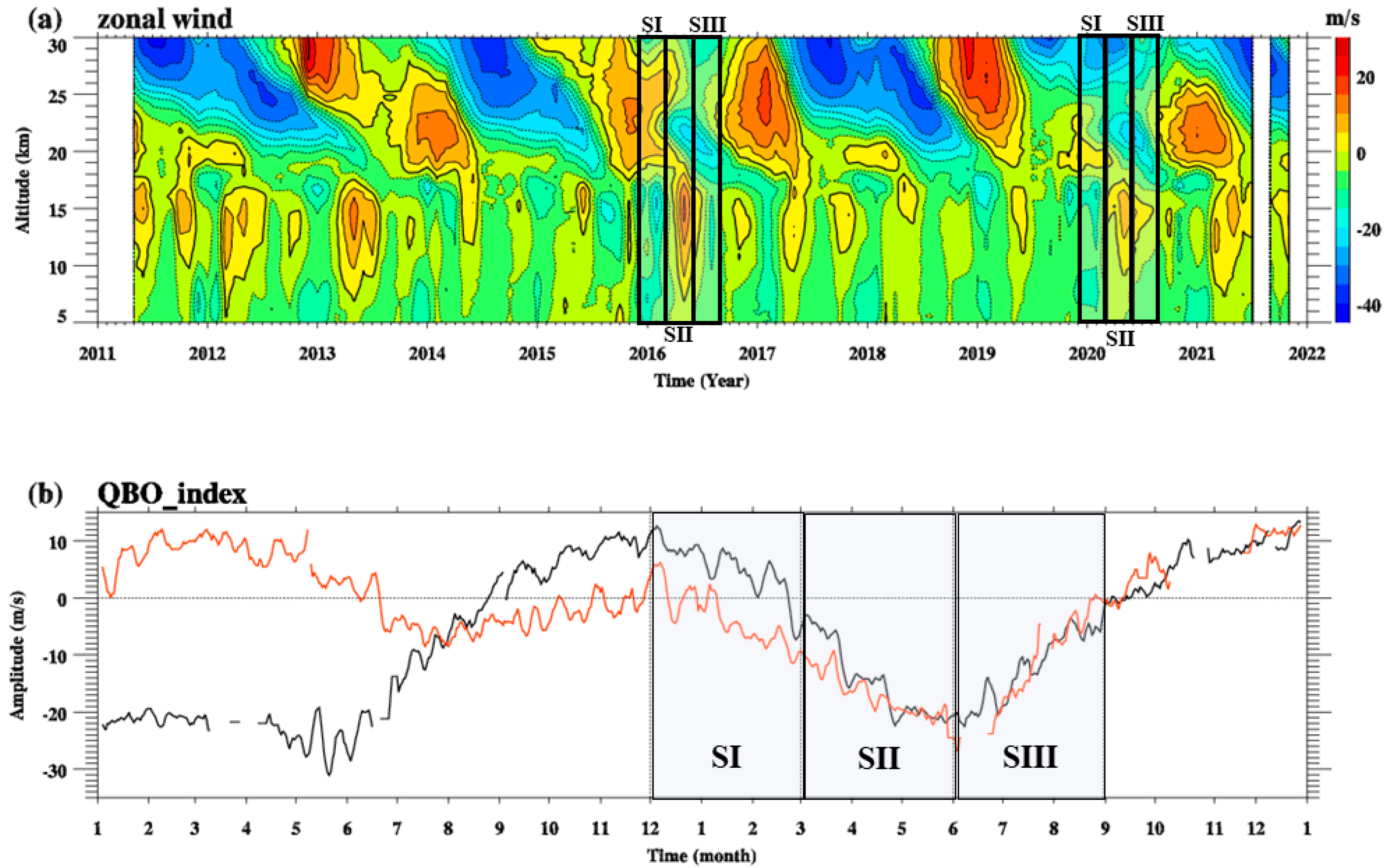
3.1. The Definition of Different Stages for the unQBO Events

Figure 1a shows that the westerly zonal wind started to turn easterly in February 2016 and January 2020 at about 22 km (corresponding to 38 hPa), which is in agreement with previous studies [15,16,20]. The zonal wind averaged within the altitude interval of 21–23 km (corresponding to 46–31 hPa), which is recognized as the QBO index in this study, as shown in Figure 1b. Notably, the QBO indexes of the 2015/2016 and 2019/2020 unQBO events had similar temporal variations from August 2015 and August 2019 in both events. The maximum amplitude (about 12.6 m/s) of the QBO index occurred in December 2015 during the 2015/2016 unQBO event. However, for the 2019/2020 unQBO event, the QBO index was small (around 0 m/s) from August 2019 to January 2020, and the maximum value (about 7.49 m/s) of the QBO index occurred in December 2019. From August 2015 to March 2016, the QBO index was larger than that from August 2019 to March 2020. From April to December 2016 and 2020, the QBO indexes had similar amplitude and temporal variations.

Figure 1b shows that the QBO index started to decrease from about 12.6 m/s (7.49 m/s) in December 2015 (2019) to about 0 m/s in February 2016 (January 2020). The period from December 2015 (2019) to February 2016 (2020) is regarded as the first stage of the unQBO events (hereinafter, SI). From March 2016 (2020), the QBO index changed into an easterly phase, and the easterly zonal wind reached the maximum amplitude in late May 2016 (2020), with a value of −25.6 m/s (−24.5 m/s). Therefore, the period of March, April, and May 2016 (2020) is defined as the easterly zonal wind developing period (hereinafter, SII). The easterly zonal wind started to decrease from June 2016 (2020). It reached about 0 m/s in late August 2016 (2020); therefore, June, July, and August 2016 (2020) is defined as the westerly zonal wind recovery period (hereinafter, SIII). These three stages of the unQBO events in 2015/2016 and 2019/2020 are marked in Figure 1b by vertical lines.

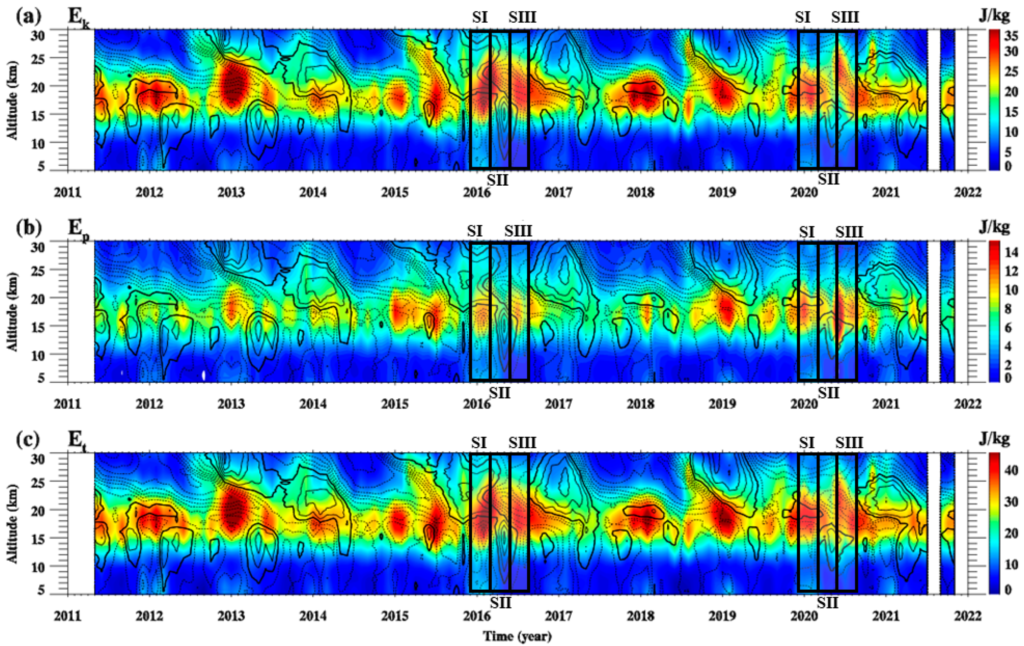
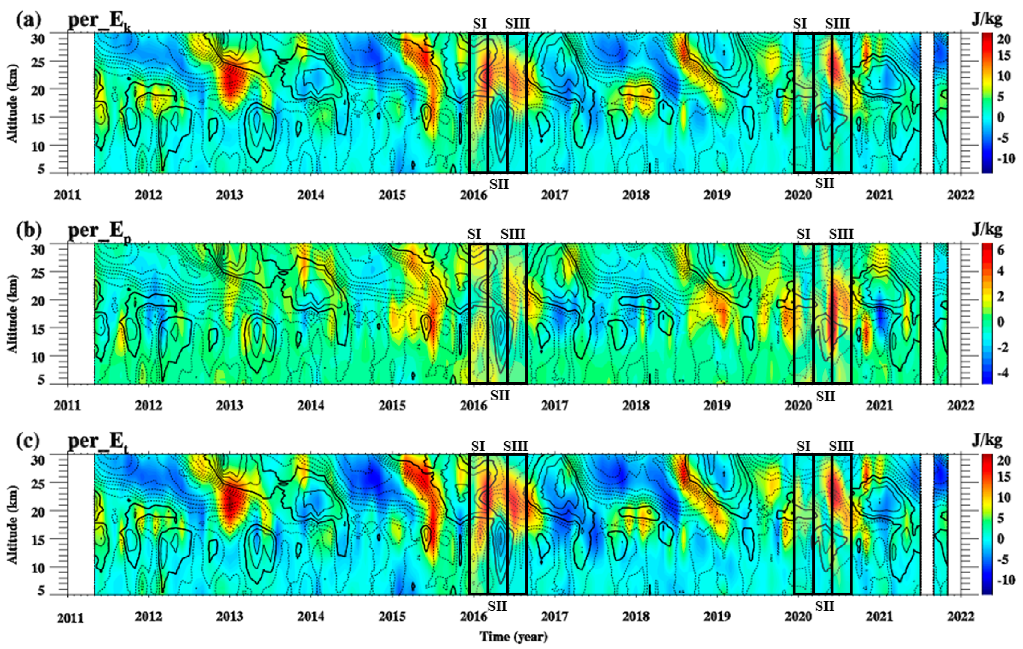
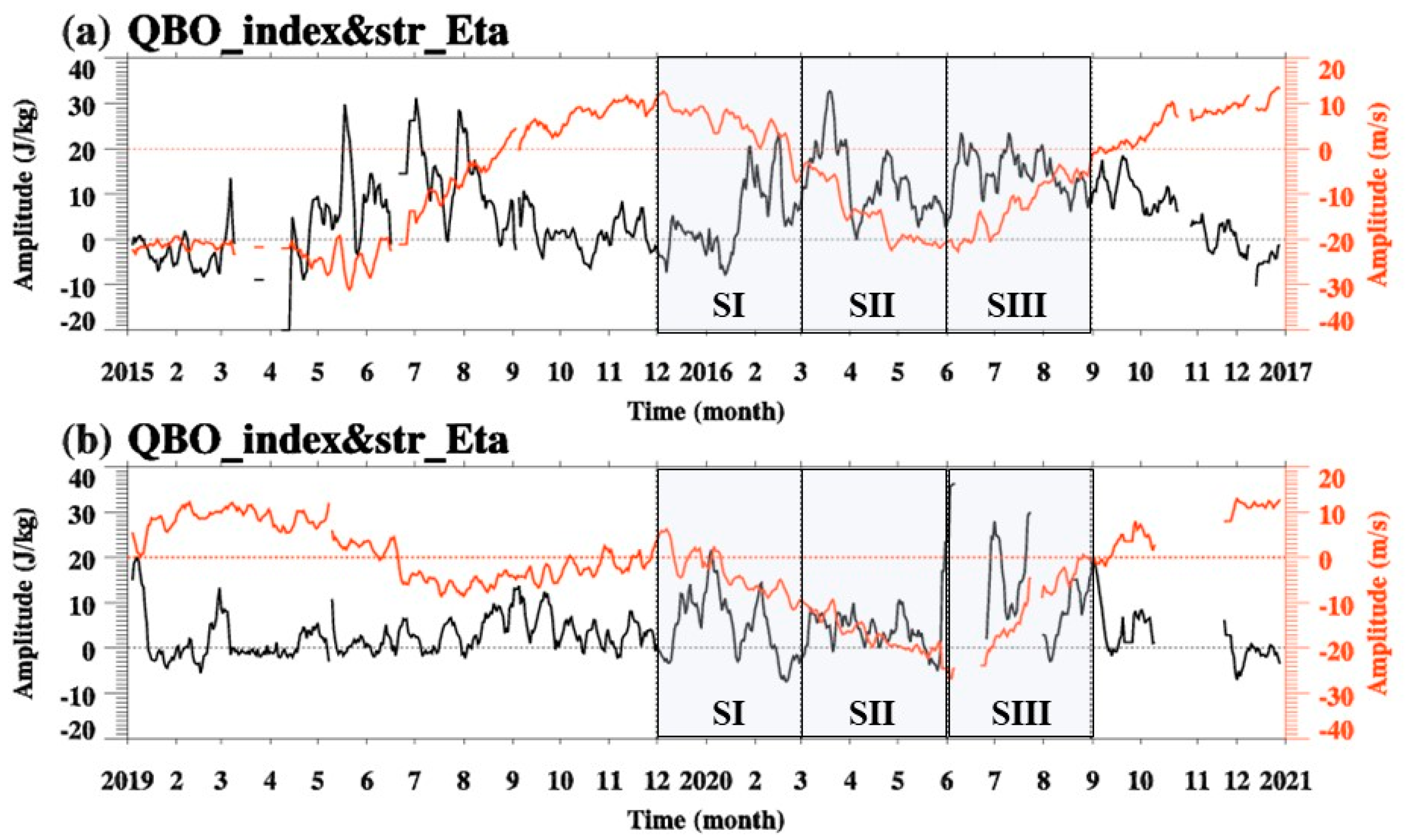
3.2. The Behavior of Stratospheric Gravity Waves during the unQBO Events

The GWs’ perturbation components in the zonal wind, meridional wind, vertical ascent rate, and temperature are extracted by using the abroad spectral method. The GWs’ zonal kinetic energy density (E_ku), meridional kinetic energy density (E_kv), kinetic energy density (E_k), potential energy density (E_p), and total energy density (E_t) are computed using Equations (1)–(5). The activity of the stratospheric GWs during the unQBO events is discussed in this section.

The monthly mean GWs’ energy densities (E_k, E_p, and E_t) within the period from 2011 to 2021 in the altitude range from 5 km to 30 km are plotted in Figure 2. E_k is much stronger than E_p but smaller than E_t. Below the height of 12 km, all the GWs’ energy densities are weak. Within the altitude range of 12–18 km (corresponding to 197–67 hPa), the GWs’ energy densities increase with altitude. The GWs’ energy densities have maxima values at around the tropopause region (about 18 km), which confirms that the tropopause region is one of the crucial sources of GWs [33,34,62]. From 18 km up to 30 km, the GWs’ energy densities are dominated by the QBO, indicating that the activity of the GWs has a close relationship with background zonal wind, which has been reported in previous studies [33,34,62,63].

To demonstrate the GW behavior during the unQBO events, we calculate the anomalies of E_k, E_p, and E_t with respect to the climatology (shown in Figure 3). Figure 3 shows that the anomalies of E_k, E_p, and E_t are weaker below 10 km. The E_k anomaly is stronger in the altitude range from 20 km to 25 km, and the maximum value is about 20 J/kg, which occurred in December 2012 at around 22 km. The E_p anomaly is stronger around the tropopause regions, and the maximum value is about 6 J/kg, which occurred in late May in the tropopause region. Due to the amplitude of the E_p anomaly being much weaker than that of the E_k anomaly, the variation in the E_t anomaly is much more similar to that in the E_t anomaly. Figure 3 shows that the GWs’ energy densities are enhanced when the zonal wind turns into a westly phase from an easterly phase in the stratosphere. When the westerly zonal wind turns into an easterly phase, the GWs’ energy densities do not generally enhance [63]. The amplitudes of the GWs’ energy densities are typically weak when the zonal wind is strong in both the westerly QBO and easterly QBO phases due to the filter effect of the background zonal wind. As shown in Figure 3a,c, the GWs’ energy densities during all stages in both unQBO events are stronger than those in regular QBO periods. In particular, in the SI stages of the 2015/2016 and 2019/2020 events, the zonal wind turns into an easterly phase from a westerly phase corresponding to the enhancement of the GWs’ energy densities, which is different from the behavior of GWs in general QBO structures.

The averaged E_t anomaly from 21 km to 23 km was calculated to represent the variations in the stratospheric GWs’ energy densities. The amplitude of the stratospheric E_t anomaly had a peak (23.5 J/kg) in February 2016, corresponding to the westerly zonal wind turning into an easterly phase. A similar result was observed in the 2019/2020 event, and a stratospheric E_t anomaly peak (21.3 J/kg) occurred in January 2020 when the westerly zonal wind turned into an easterly phase. Previous research [63] has reported that the GWs’ energy densities do not significantly enhance when the westerly zonal wind turns into an easterly phase. In contrast, the GWs’ energy densities are enhanced considerably when the westerly zonal wind turns into an easterly phase during the SI stage in both unQBO events.

As shown in Figure 4, during the SII stage, the GWs’ energy densities are enhanced in both unQBO events. Figure 4a indicate that the amplitude of the stratospheric E_t anomaly peaks in March 2016 with an amplitude of 32.7 J/kg. During the SII stage in 2020, the amplitude of the stratospheric E_t anomaly is weaker than that in the 2016 SII period. In the SIII stages in both 2015/2016 and 2019/2020, the amplitude of the stratospheric E_t anomaly is enhanced, which corresponds to the easterly zonal wind turning westerly like in the general QBO structures. The possible reasons for the enhanced GWs’ energy densities are investigated in Section 3.3.

3.3. Possible Sources of the Enhanced Gravity Waves during the unQBO Events

In this section, we identify the possible reasons for the enhanced GWs’ energy densities during the 2015/2016 and 2019/2020 unQBO events. The potential sources we explore include the tropospheric convection, tropospheric jet, and stratospheric vertical shear.

3.3.1. The Tropospheric Convection

The Outgoing Longwave Radiation (OLR) represents the tropospheric convection in this study. A decreased OLR indicates an increased tropospheric convection [17,33]. To describe the tropospheric convection, we calculate the daily mean detrended OLR during the 2015/2016 and 2019/2020 unQBO periods. The correlation coefficient between the daily mean stratospheric E_t anomaly and the detrended OLR during each stage in the 2015/2016 and 2019/2020 unQBO events are calculated. The correlation coefficients between the stratospheric E_t anomaly and the detrended OLR are significantly correlated during the SII stage in the 2015/2016 event, with correlation coefficients of −0.38. This result (shown in Figure 5c,f,i) implies that the tropospheric convection contributed to the enhanced stratospheric GWs in the 2015/2016 SII stage, which is in agreement with that of previous studies [47,48]. The negative correlation coefficients imply that the increased tropospheric convection is one of the sources of the GWs. However, the enhanced stratospheric GWs in the 2015/2016 SI and SIII stages have little relation to the tropospheric convection activity due to their small correlation coefficients. Figure 6c,f,i show the scatter plots between the stratospheric E_t anomaly and the detrended OLR in the 2019/2020 SI, SII, and SIII stages. We find that the detrended OLR only has a significant correlation with the stratospheric E_t anomaly in the SI stage in the 2019/2020 event, with a correlation coefficient value of 0.38. This positive correlation coefficient means that an increased tropospheric convection decreased the stratospheric GWs during the SI stage in 2019/2020. The correlation between the detrended OLR and the stratospheric E_t anomaly results suggests that the tropospheric convection may be a critical source of the enhanced GWs only during the SII stage in 2015/2016.

3.3.2. The Atmospheric Jet and Vertical Shear

Based on the GW theory, the atmospheric jet and vertical shear play essential roles in GW excitation [34]. The maximum amplitude of horizontal wind is recognized as a proxy for tropospheric jet sources, which is around the altitude from 13 km to 17 km around 6.79°N in the study. Then, the averaged horizontal wind from 13 km to 17 km is regarded as the tropospheric jet in the following analysis. The horizontal wind is specified by $Jet=\sqrt{{(u)}^2+{(v)}^2}$, where $u$ and $v$ are the background zonal wind and meridional winds, respectively. To eliminate the seasonal variation effect, we calculate the anomalies of the tropospheric jet from the climatology. The scatterplots of the tropospheric jet anomaly and stratospheric E_t anomaly during each stage in 2015/2016 and 2019/2020 are plotted in Figure 5 and Figure 6. Furthermore, the correlation coefficients between the tropospheric jet anomaly and the stratospheric E_t anomaly are in Figure 5 and Figure 6. The correlation coefficients are 0.64 and 0.43 during the SI and SII stages in 2015/2016, respectively, with a significant level larger than 95%. In the 2019/2020 SI and SII stages, the correlation coefficients between the tropospheric jet anomaly and the stratospheric E_t anomaly are 0.7 and 0.544, respectively. These high correlation coefficients indicate that the tropospheric jet is one of the critical sources of the enhanced stratospheric GWs during the SI and SII stages in the 2015/2016 and 2019/2020 unQBO events. However, during the SIII stages, the correlation coefficients are 0.2 and 0.221 in the 2015/2016 and 2019/2020 unQBO events, which implies that the tropospheric jet has less contribution to the enhanced stratospheric GWs during the SIII stages.

The atmospheric vertical wind shear has a close relationship with the atmospheric wave activity [28,67,68]. Therefore, we investigate the atmospheric vertical shear ($Sh$) during the 2015/2016 and 2019/2020 unQBO events in the radiosonde station latitude (about 6.97°N). We calculate the anomalies of the vertical shear of the horizontal wind ($Sh$). The vertical shear can be derived from Equation (7):

$$Sh=\sqrt{{\left(\frac{\partial u}{\partial z}\right)}^2+{\left(\frac{\partial v}{\partial z}\right)}^2}$$

(6)

The vertical shear anomaly is significantly enhanced when the zonal wind turns into westerly zonal wind from easterly zonal wind, while the enhancement is not obvious when the westerly zonal wind changes into easterly zonal wind. The variability of the vertical shear anomaly agrees with the behavior of the stratospheric GWs’ energy densities [45,47,48,63]. During the unQBO periods, the vertical shear anomaly is significantly enhanced in the easterly and westerly regimes in the stratosphere. The enhanced vertical shear anomaly corresponds to the regions with a stronger GW energy density anomaly. The stratospheric vertical shear anomaly averaged at 21–23 km (corresponding to 46–31 hPa).

In addition, we investigate the effect of the stratospheric shear anomaly on the stratospheric GW variations during each stage. The correlation coefficients between the stratospheric vertical shear anomaly and the stratospheric E_t anomaly are high in the 2015/2016 SI stage, with a value of −0.72. In the 2019/2020 SI and SII stages, the correlation coefficients are very small, and the correlation coefficient is larger in the SIII stage, with a value of −0.42. This result implies that the stratospheric vertical shear made an essential contribution to the stratospheric GWs during the 2015/2016 SI and 2019/2020 SIII stages. The results suggest that the tropospheric convection, tropospheric jet, and stratospheric vertical shear have a close relationship with the stratospheric GW variations during each stage in both unQBO events. Therefore, we quantitatively analyze the contribution of each factor to the temporal variations in the stratospheric GWs by adopting a regression analysis.

3.4. Contributions of Individual Factors

The above analysis indicates that the three factors (namely, the tropospheric convection, tropospheric jet, and stratospheric vertical shear) have a close relationship with the stratospheric GW variations during both disruption events. The contribution of each factor to the stratospheric GW activity in each stage is quantified by using a statistical regression analysis. Considering that the sample data points are few (less than 100) during the period of each stage and that there may be a correlation between the variable factors, we adopt partial least squares regression (PLSR) to estimate the contributions of each factor. The PLSR provides a method for the regression modeling of multiple dependent variables to multiple independent variables when the independent variables have less than 200 samples and when the variables have a high degree of correlation. The PLSR model is reliable, and the overall conclusion is robust. The stratospheric E_t anomaly is taken as the dependent variable, and the tropospheric jet anomaly, the stratospheric vertical shear anomaly, and the detrended OLR are taken as the independent variables to construct the PLSR model during each stage. These three independent variables can explain 71.4% (55.4%), 27.1% (38.3%), and 7.1% (11.7%) of the total variance of the stratospheric E_t anomaly during the SI, SII, and SIII stages in the 2015/2016 (2019/2020) disruption event, respectively. This result implies that at least one of the major variables for the stratospheric GW activity is captured by the PLSR model during the SI and SII stages in both events. These three factors are not essential sources for the enhanced stratospheric GWs during the SIII stage in both disruption events. Considering the minimal explanation of these three factors in the SIII stage in both events, we only analyze the SI and SII stages in the following analysis.

The standardized coefficients of the three independent variables are shown in Figure 7. The standardized regression coefficients are the regression coefficients obtained after the standardization of the independent variable, and the data are standardized to eliminate the influences of dimensional and magnitude so that different variables are comparable; therefore, the standardized regression coefficient can be used to compare the effect of different independent variables on the dependent variable. A larger standardized regression coefficient means that the dependent variable is more important to the independent variable. We find that, during the 2015/2016 SI period, the tropospheric jet anomaly significantly positively affects the stratospheric E_t anomaly. The stratospheric vertical shear significantly negatively affects the stratospheric GW variation. Only the tropospheric jet anomaly greatly positively affects the stratospheric E_t anomaly during the 2019/2020 SI period. The effects of the stratospheric vertical shear anomaly and the detrended OLR anomaly are insignificant. During the SII stages in 2015/2016 and 2019/2020, the tropospheric jet anomaly has the most significant positive effect on the stratospheric E_t anomaly.

Furthermore, the variable importance in the projection (VIP) of the three variables is plotted in Figure 8. The VIP value means that the influence of the content of each metabolite component on the classification and interpretation ability of the sample can be measured. The threshold is usually set to 1. When the VIP value is larger than 1, then it means that the factor makes an important contribution to the regression model. During the 2015/2016 SI period, the tropospheric jet anomaly and the stratospheric vertical shear anomaly are vital for the stratospheric E_t anomaly, with VIP values larger than 1. During the 2015/2016 SII period, the effect of the tropospheric jet anomaly and the detrended OLR is vital for the enhanced GWs. During the 2019/2020 SI and SII stages, only the tropospheric jet anomaly VIP value is larger than 1, which means that the tropospheric jet anomaly is important for the enhanced stratospheric GWs.

Based on the PLSR results, these three possible sources are essential in the SI and SII stages in both events. The tropospheric jet anomaly is vital for the enhanced stratospheric GWs during the SI and SII stages in both events. The stratospheric vertical shear anomaly and the detrended OLR anomaly are only important in the SI and SII stages in 2015/2016, respectively.

4. Conclusions

The regular QBO structure was disrupted in the winters of 2015/2016 and 2019/2020. We analyzed the GW activity during the QBO disruption events in detail by separating the disruption events into three stages. We analyzed the possible sources of the enhanced GWs during each stage in both events. A correlation analysis shows that the tropospheric jet, the stratospheric shear, and the OLR are closely related to the stratospheric GW energy density anomaly. The PLSR model fit the variations of the stratospheric E_t anomaly very well and could explain more than 50% and 20% of the stratospheric GWs variations in the SI and SII stages in both events. The PLSR model standardized coefficients and variable importance projection results indicate that the tropospheric jet anomaly is important during the SI and SII stages in the 2015/2016 and 2019/2020 events. The stratospheric vertical shear is important in the SI stage, and the detrended OLR is important during the SII stages in 2015/2016. The tropospheric jet and stratospheric atmospheric instability are important for the enhanced stratospheric GWs during the SI and SII stages in 2015/2016. The increased tropospheric jet should be an important source for the enhanced stratospheric GWs during the SI and SII stages in 2019/2020. Previous studies have confirmed that the subtropical jet and polar vortex have a close relationship with the QBO phase. The subtropical jet has a poleward shift during the easterly QBO phase and has a equatorward shift during the westerly QBO phase [69]. The Northern Hemispheric polar vortex is weakened/enhanced in the lower stratosphere during the easterly QBO/westerly QBO phase in winter [11]. The poleward or equatorward shift of the atmospheric jet could affect atmospheric wave propagation and momentum deposition, which can influence the QBO structure. The role of the atmospheric jet during the QBO disruption events will be explored in our future work.

References

1. Baldwin, M.P.; Gray, L.J.; Dunkerton, T.J.; Hamilton, K.; Haynes, P.H.; Holton, J.R.; Alexander, M.J.; Hirota, I.; Horinouchi, T.; Jones, D.B.A.; et al. The Quasi-Biennial Oscillation. Rev. Geophys. 2001, 39, 179–229. [Google Scholar] [CrossRef]
2. Lindzen, R.S.; Holton, J.R. A theory of the quasi-biennial oscillation. J. Atmos. Sci. 1968, 25, 1095–1107. [Google Scholar] [CrossRef]
3. Holton, J.R.; Lindzen, R.S. An update theory for the Quasi-Biennial cycle of the Tropical Stratosphere. J. Atmos. Sci. 1972, 29, 1076–1080. [Google Scholar] [CrossRef]
4. Kawatani, Y.; Hamilton, K. Weakened stratospheric quasi-biennial oscillation driven by increased tropical mean upwelling. Nature 2013, 497, 478–481. [Google Scholar] [CrossRef] [PubMed]
5. Reed, R.J.; Cambell, W.J.; Rasmussen, L.A.; Rogers, D.G. Evidence of a downward-propagating, annual wind reversal in the equatorial stratosphere. J. Geophys. Res. 1961, 66, 813–818. [Google Scholar] [CrossRef]
6. Ebdon, R.A. Notes on the wind flow at 50mb in tropical and subtropical regions in January 1957 and January 1958. Q. J. R. Meteorol. Soc. 1960, 86, 540–542. [Google Scholar] [CrossRef]
7. Gray, L.J.; Crooks, S.; Pascoe, C.; Sparrow, S.; Palmer, M. Solar and QBO Influence on the Timing of Stratospheric Sudden Warmings. J. Atmos. Sci. 2004, 61, 2777–2796. [Google Scholar] [CrossRef]
8. Yoo, C.; Son, S.W. Modulation of the boreal winter-time Madden-Julian oscillation by the stratospheric quasi-biennial oscillation. Geophys. Res. Lett. 2016, 43, 1392–1398. [Google Scholar] [CrossRef] [Green Version]
9. Holton, J.R.; Austin, J. The influence of the Equatorial QBO on Sudden Stratospheric Warmings. J. Atmos. Sci. 1991, 48, 607–618. [Google Scholar] [CrossRef]
10. Holton, J.R.; Tan, H.-C. The influence of the Equatorial Quasi-Biennial Oscillation on the Global Circulation at 50 mb. J. Atmos. Sci. 1980, 37, 2200–2208. [Google Scholar] [CrossRef]
11. Zhang, J.; Xie, F.; Ma, Z.; Zhang, C.; Xu, M.; Wang, T.; Zhang, R. Seasonal evolution of the quasi-biennial oscillation impact on the Northern Hemisphere polar vortex in winter. J. Geophys. Res. Atmos. 2019, 124, 12568–12586. [Google Scholar] [CrossRef]
12. Dunkerton, T. The role of gravity waves in the quasi-biennial oscillation. J. Geophys. Res. 1997, 102, 26053–26076. [Google Scholar] [CrossRef]
13. Kawatani, Y.; Sato, K.; Dunkerton, S.; Watanabe, S.; Miyahara, S.; Takahashi, M. The roles of equatorial trapped waves and internal gravity waves in driving the quasi-biennial oscillation. Part I: Zonal mean wave forcing. J. Atmos. Sci. 2010, 67, 963–980. [Google Scholar] [CrossRef] [Green Version]
14. Kawatani, Y.S.; Watanabe, S.; Sato, K.; Dunkerton, T.J.; Miyahara, S.; Takahashi, M. The roles of equatorial trapped waves and internal inertial-gravity waves in driving the quasi-biennial oscillation. Part II: Three-dimensional distribution of wave forcing. J. Atmos. Sci. 2010, 67, 981–997. [Google Scholar] [CrossRef] [Green Version]
15. Newman, P.A.; Coy, L.; Pawson, S.; Lait, L.R. The anomalous changes in the QBO in 2015-2016. Geophys. Res. Lett. 2016, 43, 8791–8797. [Google Scholar] [CrossRef]
16. Osprey, S.M.; Butchart, N.; Knight, J.R.; Scaife, A.A.; Hamilton, K.; Anstey, J.A.; Zhang, C. An unexpected disruption of the atmospheric quasi-biennial oscillation. Science 2016, 4156, 441–444. [Google Scholar] [CrossRef] [Green Version]
17. Li, H.; Kedzierski, R.P.; Matthes, K. On the forcings of the unusual Quasi-Biennial Oscillation structure in February 2016. Atmos. Chem. Phys. 2020, 20, 6541–6561. [Google Scholar] [CrossRef]
18. Naujokat, B. An Update of the Observed Quasi-Biennial Oscillation of the Stratospheric Winds over the Tropics. J. Atmos. Sci. 1986, 43, 1873–1877. [Google Scholar] [CrossRef]
19. Dunderton, T.J. The quasi-biennial oscillation of 2015-2016: Hiccup or death spiral? Geophys. Res. Lett. 2016, 43, 10547–10552. [Google Scholar]
20. Coy, L.; Newman, P.A.; Pawson, S.; Lait, L.R. Dynamics of the disrupted 2015/2016 quasi-biennial oscillation. J. Clim. 2017, 30, 5661–5674. [Google Scholar] [CrossRef]
21. Tweedy, O.V.; Kramarova, N.A.; Strahan, S.E.; Newman, P.A.; Coy, L.; Randel, W.J.; Park, M.; Raugh, D.W.; Frith, S.M. Response of trace gases to the disrupted 2015-2016 quasi-biennial oscillation. Atmos. Chem. Phys. 2017, 17, 6813–6823. [Google Scholar] [CrossRef]
22. Matthias, V.; Ern, M. On the origin of the mesospheric quasi-stationary planetary waves in the unusual Arctic winter 2015/2016. Atmos. Chem. Phys. 2018, 18, 4803–4815. [Google Scholar] [CrossRef] [Green Version]
23. Lin, P.; Held, I.; Ming, Y. The Early Development of the 2015/16 Quasi-Biennial Disruption. J. Atmos. Sci. 2019, 76, 821–836. [Google Scholar] [CrossRef]
24. Barton, C.A.; McCormack, J.P. Origin of the 2016 QBO Disruption and Its Relationship to Extreme El Nino Events. Geophys. Res. Lett. 2017, 44, 11150–11157. [Google Scholar] [CrossRef]
25. Kumar, K.K.; Mathew, S.S.; Subrahmanyam, K.V. Anomalous tropical planetary wave activity during 2015/2016 quasi biennial oscillation disruption. J. Atmos. Sci. 2018, 167, 184–189. [Google Scholar] [CrossRef]
26. Hirota, N.; Shiogama, H.; Akiyoshi, H.; Ogura, T.; Takahashi, M.; Kawatani, Y.; Kimoto, M.; Mori, M. The influence of El Nino and Arctic sea-ice on the QBO disruption in February 2016. NPJ Clim. Atmos. Sci. 2018, 1, 10. [Google Scholar] [CrossRef] [Green Version]
27. Lindzen, R.S. Turbulence and stress owing to gravity wave and tidal breakdown. J. Geophys. Res. 1981, 86, 9707–9714. [Google Scholar] [CrossRef] [Green Version]
28. Fritts, D.C.; Rastogi, P.K. Convective and dynamical instabilities due to gravity wave motion in the lower and middle atmosphere: Theory and observations. Radio Sci. 1985, 20, 1247–1277. [Google Scholar] [CrossRef]
29. Alexander, M.J.; Pfister, L. Gravity wave momentum flux in the lower stratosphere over convection. Geophys. Res. Lett. 1995, 22, 2029–2032. [Google Scholar] [CrossRef] [Green Version]
30. Alexander, M.J. Interpretations of observed climatological patterns in stratospheric gravity wave variance. J. Geophys. Res. 1998, 103, 8627–8640. [Google Scholar] [CrossRef]
31. Zhang, S.D.; Yi, F. Latitudinal and seasonal variations of inertial gravity wave activity in the lower atmosphere over central China. J. Geophys. Res. 2007, 112, D05109. [Google Scholar] [CrossRef]
32. Zhang, S.D.; Yi, F.; Huang, C.M.; Chen, Z.Y. Intensive radiosonde observations of gravity waves in the lower atmosphere over Yichang (111°18’E, 30°42’N), China. Ann. Geophys. 2008, 26, 2005–2018. [Google Scholar] [CrossRef] [Green Version]
33. Zhang, S.D.; Yi, F.; Huang, C.M.; Huang, K.M. High vertical resolution analyses of gravity waves and turbulence at a midlatitude station. J. Geophys. Res. 2012, 117, D02013. [Google Scholar] [CrossRef] [Green Version]
34. Zhang, Y.; Zhang, S.D.; Huang, C.M.; Huang, K.M.; Gong, Y. The tropopause Inversion Layer Interaction with Inertial Gravity Wave Activities and Its Latitudinal Variability. J. Geophys. Res. Atmos. 2019, 124, 7512–7522. [Google Scholar] [CrossRef]
35. Scaife, A.A.; Butchart, N.; Warner, C.D.; Stainforth, D.; Norton, W. Realistic quasi-biennial oscillations in a simulation of the global climate. Geophys. Res. Lett. 2000, 27, 3481–3484. [Google Scholar] [CrossRef]
36. Giogetta, M.A.; Manzini, E.; Roeckner, E. Forcing of the quasi-biennial oscillation from a broad spectrum of atmospheric waves. Geophys. Res. Lett. 2002, 29, 861–864. [Google Scholar] [CrossRef] [Green Version]
37. Ern, M.; Preusse, P. Wave fluxes of equatorial Kelvin waves and QBO zonal wind forcing derived from SABER and ECMWF temperature space-time spectra. Atmos. Chem. Phys. 2009, 9, 3957–3986. [Google Scholar] [CrossRef] [Green Version]
38. Ern, M.; Preusse, P. Quantification of the contribution of equatorial Kelvin waves to the QBO wind reversal in the stratosphere. Geophys. Res. Lett. 2009, 36, L21801. [Google Scholar] [CrossRef] [Green Version]
39. Orr, A.; Bechtold, P.; Scinocca, J.F.; Ern, M.; Janiskova, M. Improved middle atmosphere climate and forecasts in the ECMWF model through a nonorographic gravity wave drag parameterization. J. Clim. 2010, 23, 5905–5926. [Google Scholar] [CrossRef] [Green Version]
40. Evan, S.; Alexander, M.J.; Dudhia, J. WRF simulations of convectively generated gravity waves in opposite QBO phases. J. Geophys. Res. 2012, 117, D12117. [Google Scholar] [CrossRef] [Green Version]
41. Xue, X.H.; Liu, H.L.; Dou, X.K. Parameterization of the inertial gravity waves and generation of the quasi-biennial oscillation. J. Geophys. Res. 2013, 117, D06103. [Google Scholar] [CrossRef]
42. Ern, M.; Ploeger, F.; Preusse, P.; Gille, J.C.; Gray, L.J.; Kalisch, S.; Mlynczak, M.G.; Russell III, J.M.; Riese, M. Interaction of gravity wave with QBO: A satellite perspective. J. Geophys. Res. Atmos. 2014, 119, 2329–2355. [Google Scholar] [CrossRef]
43. Ji, Q.; Zhu, X.; Sheng, Z.; Tian, T. Spectral Analysis of Gravity Waves in the Martian Thermosphere during Low Solar Activity Based on MAVEN/NGIMS Observations. Astrophys. J. 2022, 938, 97. [Google Scholar] [CrossRef]
44. Zhang, J.; Ji, Q.; Sheng, Z.; He, M.; He, Y.; Zuo, X.; He, Z.; Qin, Z.; Wu, G. Observation based climatology Martian atmospheric waves perturbation Datasets. Sci. Data 2023, 10, 4. [Google Scholar] [CrossRef] [PubMed]
45. He, Y.; Zhu, X.; Sheng, Z.; He, M.; Feng, Y. Observations of inertia gravity waves in the western Pacific and their characteristic in the 2015/2016 quasi-biennial oscillation disruption. J. Geophys. Res. Atmos. 2022, 127, e2022JD037208. [Google Scholar] [CrossRef]
46. Anstey, J.A.; Banyard, T.P.; Butchart, N.; Coy, L.; Newman, P.A.; Osprey, S.; Wright, C.J. Prospect of increased disruption to the QBO in a changing climate. Geophys. Res. Lett. 2021, 48, e2021GL093058. [Google Scholar] [CrossRef]
47. Kang, M.; Chun, H.-Y.; Garcia, R.R. Role of equatorial waves and convective gravity waves in the 2015/2016 quasi-biennial oscillation disruption. Atmos. Chem. Phys. 2020, 20, 14669–14693. [Google Scholar] [CrossRef]
48. Kang, M.-J.; Chun, H. Contributions of equatorial waves and small-scale convective gravity waves to the 2019/2020 quasi-biennial oscillation (QBO) disruption. Atmos. Chem. Phys. 2021, 21, 9839–9857. [Google Scholar] [CrossRef]
49. Geller, M.A.; Alexander, M.J.; Love, P.T.; Bacmeister, J.; Ern, M.; Hertzog, A.; Manzini, E.; Preusse, P.; Sato, K.; Scaife, A.A.; et al. A comparison between gravity wave momentum fluxes in observations and climate models. J. Clim. 2013, 26, 6383–6405. [Google Scholar] [CrossRef] [Green Version]
50. Alexander, M.J. Global and seasonal variations in three-dimensional gravity wave momentum flux from satellite limb-sounding temperatures. Geophys. Res. Lett. 2015, 42, 6860–6867. [Google Scholar] [CrossRef] [Green Version]
51. Richter, J.H.; Solomon, A.; Bacmeister, J.T. On the simulation of the quasi-biennial oscillation in the Community Atmosphere Model, version 5. J. Geophys. Res. Atmos. 2014, 119, 3045–3062. [Google Scholar] [CrossRef]
52. Bushell, A.C.; Buchart, N.; Derbyshire, S.H.; Jackson, D.R.; Shutts, G.J.; Vosper, S.B.; Webster, S. Parameterized gravity wave momentum fluxes sources related to convection and large-scale precipitation processes in a global atmosphere model. J. Atomos. Sci. 2015, 72, 4349–4371. [Google Scholar] [CrossRef]
53. Schirber, S. Influence of ENSO on the QBO: Results from an ensemble of idealized simulations. J. Geophys. Res. 2015, 120, 1109–1122. [Google Scholar] [CrossRef] [Green Version]
54. Tsuda, T.; Murayama, Y.; Wiryosumarto, H.; Harijono, S.W.B.; Kato, S. Radiosonde observations of equatorial atmosphere dynamics over Indonesia: 2. Characteristics of gravity waves. J. Geophys. Res. 1994, 99, 10506–10516. [Google Scholar] [CrossRef]
55. Vicent, R.A.; Alexander, M.J. Gravity waves in the tropical lower stratosphere: An observational study of seasonal and inter-annual variability. J. Geophys. Res. 2000, 105, 17971–17982. [Google Scholar] [CrossRef]
56. Yoshiki, M.; Sato, K. A statistical study of gravity waves in the polar regions based on operational radiosonde data. J. Geophys. Res. 2000, 105, 17995–18011. [Google Scholar] [CrossRef]
57. Zink, F.; Vincent, R.A. Wavelet analysis of stratospheric gravity wave packets over Macquarie Island, 1. Wave parameters. J. Geophys. Res. 2001, 106, 10275–10288. [Google Scholar] [CrossRef] [Green Version]
58. Zink, F.; Vicent, R.A. Wavelet analysis of stratospheric gravity wave packets over Macquarie Island, 2. Intermittency and Meanflow accelerations. J. Geophys. Res. 2000, 106, 10289–10297. [Google Scholar] [CrossRef] [Green Version]
59. Wang, L.; Geller, M.A.; Alexander, M.J. Spatial and temporal variations of gravity wave parameters, Part I: Intrinsic frequency, wavelength, and vertical propagation direction. J. Atmos. Sci. 2005, 62, 125–142. [Google Scholar] [CrossRef]
60. Zhang, S.D.; Yi, F. A statistical study of gravity waves from radiosonde observations at Wuhan (30°N, 114°E), China. Ann. Geophys. 2005, 23, 665–673. [Google Scholar] [CrossRef] [Green Version]
61. Zhang, S.D.; Huang, C.M.; Huang, K.M.; Yi, F.; Zhang, Y.H.; Gong, Y.; Gan, Q. Spatial and seasonal variability of medium and high -frequency gravity waves in the lower atmosphere revealed by US radiosonde data. Ann. Geophys. 2014, 32, 1129–1143. [Google Scholar] [CrossRef]
62. Zhang, S.D.; Yi, F.; Huang, C.M.; Zhou, Q.H. Latitudinal and seasonal variations of lower atmospheric inertial gravity wave energy revealed by US radiosonde data. Ann. Geophys. 2010, 28, 1065–1074. [Google Scholar] [CrossRef] [Green Version]
63. Li, H.Y.; Huang, C.M.; Zhang, S.D.; Huang, K.M.; Zhang, Y.; Gong, Y.; Gan, Q.; Jia, Y. Low-frequency oscillations of the gravity wave energy density in the lower atmosphere at low latitudes revealed by U.S. radiosonde data. J. Geophys. Res. Atmos. 2016, 121, 13458–13473. [Google Scholar] [CrossRef]
64. Zhang, S.D.; Yi, F.; Huang, C.M.; Huang, K.M.; Gan, Q.; Zhang, Y.H.; Gong, Y. Latitudinal and altitudinal variability of lower atmospheric inertial gravity waves revealed by U.S. radiosonde data. J. Geophys. Res. Atmos. 2013, 118, 7750–7764. [Google Scholar] [CrossRef]
65. Gong, J.; Geller, M.A. Vertical fluctuation energy in United States high vertical resolution radiosonde data as an indicator of convective gravity wave sources. J. Geophys. Res. 2010, 115, D11110. [Google Scholar] [CrossRef]
66. Zhang, J.; Guo, J.; Xue, H.; Zhang, S.; Huang, K.; Dong, W.; Shao, J.; Yi, M.; Zhang, Y. Tropospheric Gravity Waves as observed by the High-Resolution China Radiosonde Network and Their Potential Sources. J. Geophys. Res. Atmos. 2022, 127, e2022JD037174. [Google Scholar] [CrossRef]
67. Liu, H.-L. Large wind shears and their implications for diffusion in regions with enhanced staic stability: The mesopause and the tropopause. J. Geophys. Res. Atmos. 2017, 122, 9579–9590. [Google Scholar] [CrossRef]
68. Fritts, D.C.; Alexander, M.J. Gravity wave dynamics and effects in the middle atmosphere. Rev. Geophys. 2003, 41, 1003. [Google Scholar] [CrossRef] [Green Version]
69. Lachmy, O.; Harnik, N. The Transition to a Subtropical Jet Regime and Its Maintenance. J. Atmos. Sci. 2014, 71, 1389–1409. [Google Scholar] [CrossRef]
Figure 1. (a) Temporal evolution of monthly zonal wind over Ponape Island station (6.97°N, 158.22°E). Panel (b) denotes the daily time series of the averaged zonal wind from 21 km to 23 km over Ponape Island station (6.97°N, 158.22°E) in 2015/2016 (black line) and 2019/2020 (red line). The solid and dotted contours denote the eastward and westward winds, respectively, with a contour interval of 5 m/s in (a). The thick contours represent zero zonal wind. The blanks denote no observational data. The horizontal dashed line in panel (b) denotes the speed of 0 m/s. The black and red lines denote the QBO index for 2015/2016 and 2019/2020, respectively. Boxes indicate SI, SII, and SIII stages in panels (a,b).
Remotesensing 15 00472 g001
Figure 2. Altitude and temporal variations in monthly mean gravity wave (a) kinetic energy density (in J/kg), (b) potential energy density (in J/kg), and (c) total energy density (in J/kg) over Ponape Island (6.97°N, 158.22°E). The monthly mean zonal wind is overplotted in black contours with a contour interval of 5 m/s. The solid and dashed contours denote the westward and eastward zonal winds, respectively. The thick contours represent zero zonal wind. The blanks represent no observational data. Boxes indicate SI, SII, and SIII stages in panels (ac).
Remotesensing 15 00472 g002
Figure 3. Temporal evolution of gravity wave (a) kinetic energy density anomaly, (b) potential energy density anomaly, and (c) total energy density anomaly. Color shading denotes the GWs energy density anomalies with respect to the monthly climatology (the unit is J/kg). The monthly mean zonal wind is overlaid in black contours with a contour interval of 5 m/s. The solid and dashed black contours denote the eastward and westward zonal wind, respectively. The thick contours represent zero zonal wind. The blanks indicate no observational data. Boxes indicate SI, SII, and SIII stages in panels (ac).
Remotesensing 15 00472 g003
Figure 4. The time series of the QBO index and stratospheric Et anomaly over Ponape Island station (6.97°N, 158.22°E) in (a) 2015/2016 and (b) 2019/2020. The red lines denote the QBO index. The black lines indicate the stratospheric Et anomaly. The horizontal lines represent wind speed, which is 0 m/s (red line), and energy density anomaly, which is 0 J/kg (black lines). Boxes indicate SI, SII, and SIII stages.
Remotesensing 15 00472 g004
Figure 5. Panels (a,d,g) display the scatterplots between tropospheric jet anomaly and the stratospheric GW total energy density anomaly in SI, SII, and SIII stages in the 2015/2016 event, respectively. Panels (b,e,h) are similar to the panels (a,d,g) but instead display the scatterplots between stratospheric vertical shear anomaly and stratospheric GW total energy density anomaly in SI, SII, and SIII stages in 2015/2016, respectively. Panels (c,f,i) are similar to above panels but instead display the scatterplots between detrended OLR and stratospheric GW total energy density anomaly in SI, SII, and SIII in the 2015/2016 event, respectively. The lines denote the fit lines. The correlation coefficients between each factor and the stratospheric GW total energy density anomaly are displayed in the upper right corner of each panel. The double asterisk (“**”) denotes a significant level larger than 95%.
Remotesensing 15 00472 g005
Figure 6. Panels (a,d,g) display the scatterplots between tropospheric jet anomaly and the stratospheric GW total energy density anomaly in SI, SII, and SIII stages in the 2019/2020 event, respectively. Panels (b,e,h) are similar to panels (a,d,g) but instead display the scatterplots between stratospheric vertical shear anomaly and stratospheric GW total energy density anomaly in SI, SII, and SIII stages in 2019/2020, respectively. Panels (c,f,i) are similar to above panels but instead display the scatterplots between detrended OLR and stratospheric GW total energy density anomaly in SI, SII, and SIII in the 2019/2020 event, respectively. The lines denote the fit line. The correlation coefficients between each factor and the stratospheric GW total energy density anomaly are displayed in the upper right corner of each panel. The double asterisk (“**”) denotes a significant level larger than 95%.
Remotesensing 15 00472 g006
Figure 7. The standardized coefficients of the tropospheric jet (blue bars), stratospheric vertical shear (black bars), and tropospheric convection (red bars) during the (a) 2015/2016 SI stage, (b) 2015/2016 SII stage, (c) 2019/2020 SI stage, and (d) 2019/2020 SII stage.
Remotesensing 15 00472 g007
Figure 8. The variable importance in projection of the tropospheric jet (blue bars), stratospheric vertical shear (black bars), and tropospheric convection (red bars) during the (a) 2015/2016 SI stage, (b) 2015/2016 SII stage, (c) 2019/2020 SI stage, and (d) 2019/2020 SII stage.
Remotesensing 15 00472 g008
Disclaimer/Publisher’s Note: The statements, opinions and data contained in all publications are solely those of the individual author(s) and contributor(s) and not of MDPI and/or the editor(s). MDPI and/or the editor(s) disclaim responsibility for any injury to people or property resulting from any ideas, methods, instructions or products referred to in the content.