
Monitoring Land Degradation through Vegetation Dynamics Mathematical Modeling: Case of Jornada Basin (in the U.S.)
 and
and 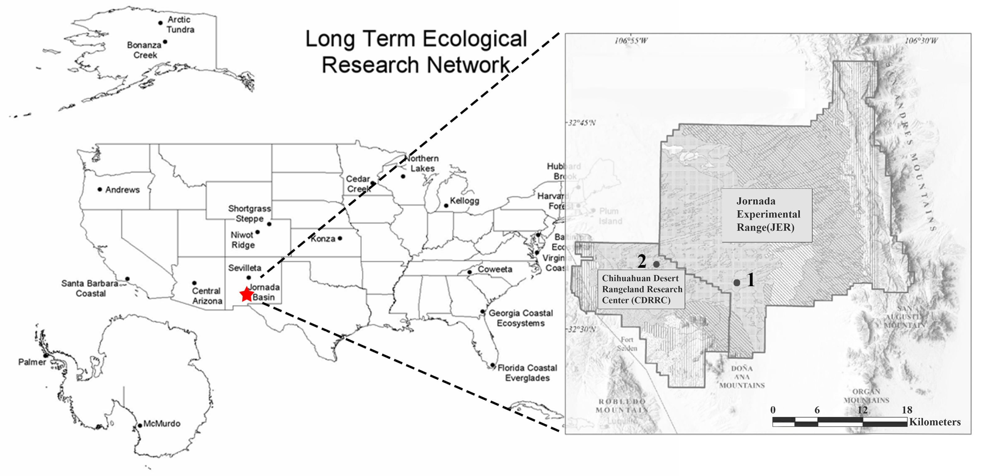
Abstract
:1. Introduction
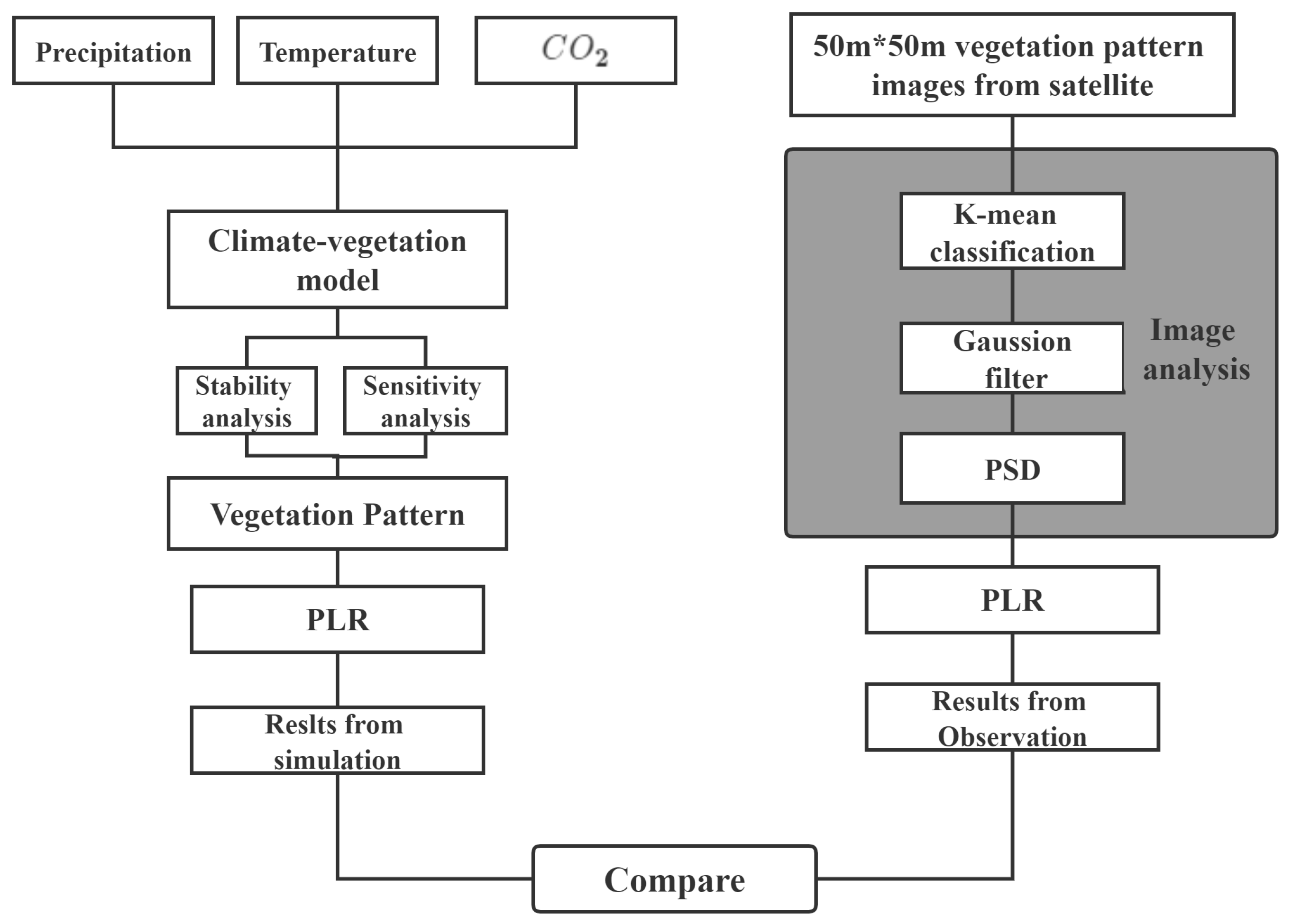
2. Materials and Methods
2.1. Study Area
2.2. Data
2.3. Image Analysis
2.4. Vegetation Patch Size Metric
2.5. Mathematical Model
3. Results
3.1. System Dynamics Implementation
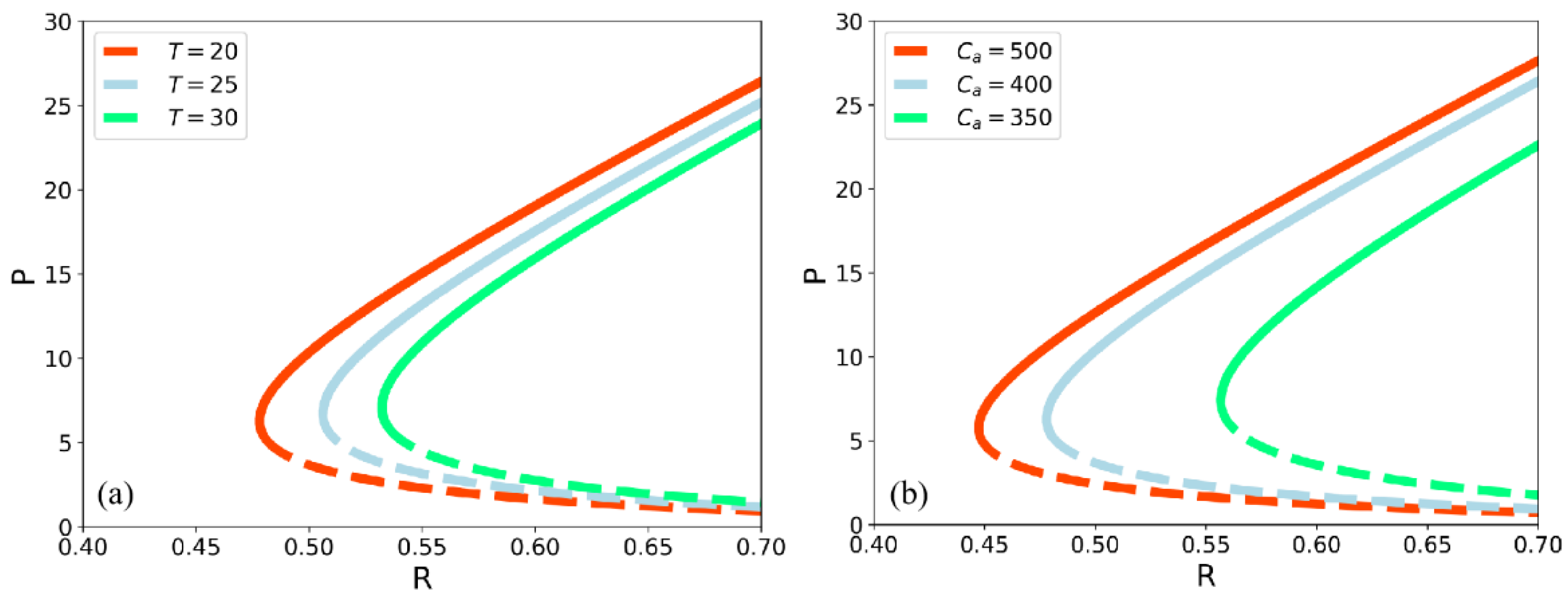
3.2. Sensitivity Analysis of the Climate Factors
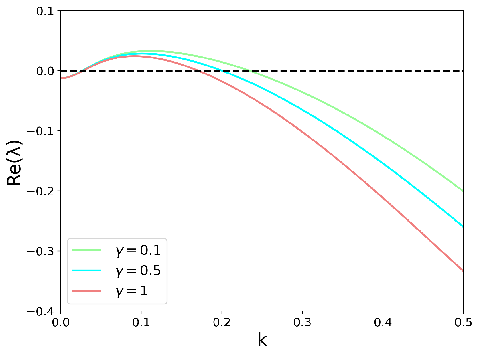
3.3. Linear Stability Analysis with a Spatial Term
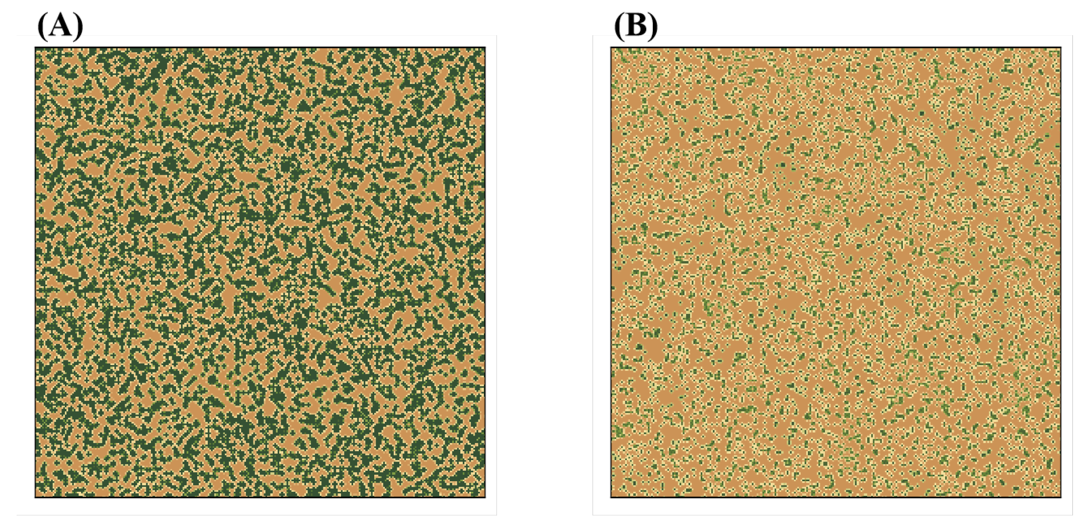
3.4. Vegetation Pattern Formation
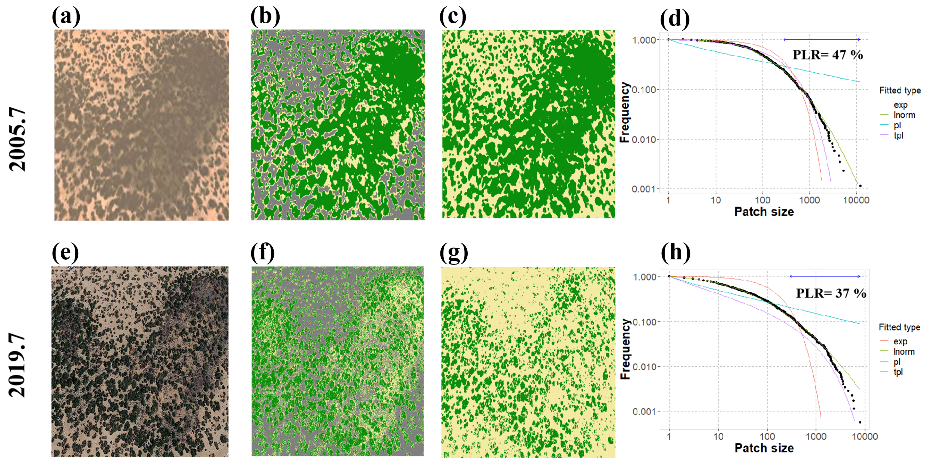
3.5. Degradation Detection
3.5.1. Detection from the Remote Sensing Data
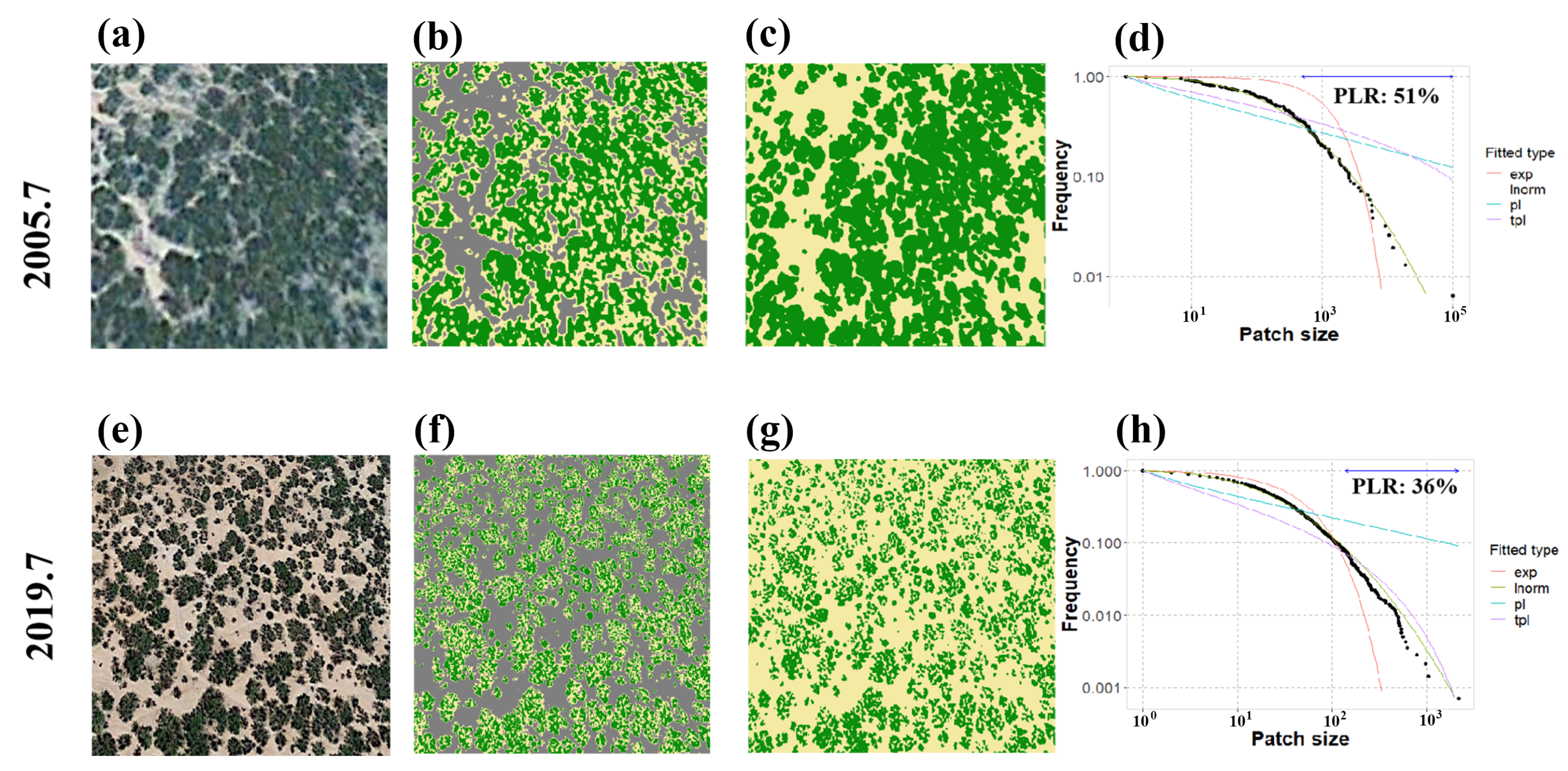
3.5.2. Detection from the Model Simulation
4. Discussion
5. Conclusions
Author Contributions
Funding
Data Availability Statement
Conflicts of Interest
Appendix A. Detailed Model Description
Appendix A.1. Dynamics of the Water Density
Appendix A.2. Dynamics of the Vegetation Biomass
Appendix B. Parameters Description
Appendix B.1. The Parameters Used in the Model
Appendix B.2. Table of Parameters
| Parameter | Interpretation | Unit |
| Half-saturation constant of specific plant growth and water uptake | mm d | |
| Saturation constant of water infiltration | g m | |
| Conversion coefficient of biomass | gm | |
| Measure of the infiltration contrast between vegetated and bare soil | d | |
| Specific soil water loss due to evaporation and drainage | d | |
| Plant dispersal | md | |
| Diffusion coefficient for soil water | md | |
| Coefficient of conversion of photosynthesis (mol) into biomass (g) | g mol | |
| Maximal leaf conductance to | mol md | |
| Conversion coefficient from maximal leaf conductance to water vapor | mm mmol | |
| to maximal leaf conductance | ||
| Ambient concentration | mol mol | |
| Intercellular concentration (in the leaf) | mol mol | |
| Respiration per unit of biomass | d | |
| Q | The factor respiration increases with a 10 degree increase in temperature | Dimensionless |
| T | Temperature | °C |
| Vapor pressure at T | kPa | |
| Saturated vapor pressure | kPa | |
| Rh | Relative humidity, | Dimensionless |
| R | Rainfall | mm d |
| P | Plant density | g m |
| W | Soil water | mm |
References
- Thackeray, C.W.; Hall, A.; Norris, J.; Chen, D. Constraining the increased frequency of global precipitation extremes under warming. Nat. Clim. Chang. 2022, 12, 441–448. [Google Scholar] [CrossRef]
- Thomas, D.S.; Knight, M.; Wiggs, G.F. Remobilization of southern African desert dune systems by twenty-first century global warming. Nature 2005, 435, 1218–1221. [Google Scholar] [CrossRef]
- Archer, S.R.; Peters, D.P.; Burruss, N.D.; Yao, J. Mechanisms and drivers of alternative shrubland states. Ecosphere 2022, 13, e3987. [Google Scholar] [CrossRef]
- Fredrickson, E.; Havstad, K.M.; Estell, R.; Hyder, P. Perspectives on desertification: South-western United States. J. Arid Environ. 1998, 39, 191–207. [Google Scholar] [CrossRef]
- Bestelmeyer, B.T.; Wiens, J.A. Scavenging ant foraging behavior and variation in the scale of nutrient redistribution among semi-arid grasslands. J. Arid Environ. 2003, 53, 373–386. [Google Scholar] [CrossRef]
- Fredrickson, E.L.; Estell, R.; Laliberte, A.; Anderson, D. Mesquite recruitment in the Chihuahuan Desert: Historic and prehistoric patterns with long-term impacts. J. Arid Environ. 2006, 65, 285–295. [Google Scholar] [CrossRef]
- Peters, D.; Havstad, K. Nonlinear dynamics in arid and semi-arid systems: Interactions among drivers and processes across scales. J. Arid Environ. 2006, 65, 196–206. [Google Scholar] [CrossRef]
- Chen, Z.; Wu, Y.; Feng, G.; Qian, Z.; Sun, G. Effects of global warming on pattern dynamics of vegetation: Wuwei in China as a case. Appl. Math. Comput. 2021, 390, 125666. [Google Scholar] [CrossRef]
- Fensham, R.; Fairfax, R.; Archer, S. Rainfall, land use and woody vegetation cover change in semi-arid Australian savanna. J. Ecol. 2005, 93, 596–606. [Google Scholar] [CrossRef]
- Gillson, L.; Hoffman, M.T. Rangeland ecology in a changing world. Science 2007, 315, 53–54. [Google Scholar] [CrossRef] [PubMed] [Green Version]
- Wendling, V.; Peugeot, C.; Mayor, A.G.; Hiernaux, P.; Mougin, E.; Grippa, M.; Kergoat, L.; Walcker, R.; Galle, S.; Lebel, T. Drought-induced regime shift and resilience of a Sahelian ecohydrosystem. Environ. Res. Lett. 2019, 14, 105005. [Google Scholar] [CrossRef]
- Yonaba, R.; Biaou, A.C.; Koïta, M.; Tazen, F.; Mounirou, L.A.; Zouré, C.O.; Queloz, P.; Karambiri, H.; Yacouba, H. A dynamic land use/land cover input helps in picturing the Sahelian paradox: Assessing variability and attribution of changes in surface runoff in a Sahelian watershed. Sci. Total Environ. 2021, 757, 143792. [Google Scholar] [CrossRef] [PubMed]
- Scott, R.L.; Huxman, T.E.; Cable, W.L.; Emmerich, W.E. Partitioning of evapotranspiration and its relation to carbon dioxide exchange in a Chihuahuan Desert shrubland. Hydrol. Process. Int. J. 2006, 20, 3227–3243. [Google Scholar] [CrossRef]
- Li, J.; Sun, G.; Guo, Z. Bifurcation analysis of an extended Klausmeier–Gray–Scott model with infiltration delay. Stud. Appl. Math. 2022, 148, 1519–1542. [Google Scholar] [CrossRef]
- Liu, J.Y.; Qiao, S.B.; Li, C.; Tang, S.K.; Chen, D.; Feng, G.L. Anthropogenic influence on the intensity of extreme precipitation in the Asian-Australian Monsoon Region in HadGEM3-A-N216. Atmos. Sci. Lett. 2021, 22, e1036. [Google Scholar] [CrossRef]
- Cramer, M.D.; Barger, N.N. Are Namibian “fairy circles” the consequence of self-organizing spatial vegetation patterning? PLoS ONE 2013, 8, e70876. [Google Scholar] [CrossRef]
- Chen, Z.; Liu, J.; Li, L.; Wu, Y.; Feng, G.; Qian, Z.; Sun, G. Effects of climate change on vegetation patterns in Hulun Buir Grassland. Phys. A Stat. Mech. Its Appl. 2022, 597, 127275. [Google Scholar]
- Kéfi, S.; Rietkerk, M.; Alados, C.L.; Pueyo, Y.; Papanastasis, V.P.; ElAich, A.; De Ruiter, P.C. Spatial vegetation patterns and imminent desertification in Mediterranean arid ecosystems. Nature 2007, 449, 213–217. [Google Scholar] [CrossRef]
- Sun, G.; Zhang, H.; Song, Y.; Li, L.; Jin, Z. Dynamic analysis of a plant-water model with spatial diffusion. J. Differ. Equ. 2022, 329, 395–430. [Google Scholar]
- Li, J.; Sun, G.; Jin, Z. Interactions of time delay and spatial diffusion induce the periodic oscillation of the vegetation system. Discret. Contin. Dyn. Syst.-B 2022, 27, 2147–2172. [Google Scholar] [CrossRef]
- Xue, Q.; Liu, C.; Li, L.; Sun, G.Q.; Wang, Z. Interactions of diffusion and nonlocal delay give rise to vegetation patterns in semi-arid environments. Appl. Math. Comput. 2021, 399, 126038. [Google Scholar] [CrossRef]
- Ji, W.; Hanan, N.P.; Browning, D.M.; Monger, H.C.; Peters, D.P.; Bestelmeyer, B.T.; Archer, S.R.; Ross, C.W.; Lind, B.M.; Anchang, J.; et al. Constraints on shrub cover and shrub–shrub competition in a US southwest desert. Ecosphere 2019, 10, e02590. [Google Scholar] [CrossRef] [Green Version]
- Havstad, K.; Schlesinger, W. Reflections on a Century of Rangeland Research in the Jornada Basin of New Mexico. In Proceedings: Shrubland Ecosystem Dynamics in a Changing Environment; United States Department of Agriculture: Ogden, UT, USA, 1996; pp. 10–15. [Google Scholar]
- Gibbens, R.; McNeely, R.; Havstad, K.; Beck, R.; Nolen, B. Vegetation changes in the Jornada Basin from 1858 to 1998. J. Arid Environ. 2005, 61, 651–668. [Google Scholar] [CrossRef]
- Maestre, F.T.; Quero, J.L.; Gotelli, N.J.; Escudero, A.; Ochoa, V.; Delgado-Baquerizo, M.; García-Gómez, M.; Bowker, M.A.; Soliveres, S.; Escolar, C.; et al. Plant species richness and ecosystem multifunctionality in global drylands. Science 2012, 335, 214–218. [Google Scholar] [CrossRef] [PubMed]
- Delgado-Baquerizo, M.; Maestre, F.T.; Gallardo, A.; Bowker, M.A.; Wallenstein, M.D.; Quero, J.L.; Ochoa, V.; Gozalo, B.; García-Gómez, M.; Soliveres, S.; et al. Decoupling of soil nutrient cycles as a function of aridity in global drylands. Nature 2013, 502, 672–676. [Google Scholar] [CrossRef] [PubMed]
- White, E.P.; Enquist, B.J.; Green, J.L. On estimating the exponent of power-law frequency distributions. Ecology 2008, 89, 905–912. [Google Scholar] [CrossRef]
- Berdugo, M.; Kéfi, S.; Soliveres, S.; Maestre, F.T. Plant spatial patterns identify alternative ecosystem multifunctionality states in global drylands. Nat. Ecol. Evol. 2017, 1, 0003. [Google Scholar] [CrossRef]
- Solomon, C.; Breckon, T. Fundamentals of Digital Image Processing: A Practical Approach with Examples in Matlab; John Wiley & Sons: Hoboken, NJ, USA, 2011. [Google Scholar]
- Otsu, N. A threshold selection method from gray-level histograms. IEEE Trans. Syst. Man Cybern. 1979, 9, 62–66. [Google Scholar] [CrossRef]
- Scanlon, T.M.; Caylor, K.K.; Levin, S.A.; Rodriguez-Iturbe, I. Positive feedbacks promote power-law clustering of Kalahari vegetation. Nature 2007, 449, 209–212. [Google Scholar] [CrossRef]
- Lin, Y.; Han, G.; Zhao, M.; Chang, S.X. Spatial vegetation patterns as early signs of desertification: A case study of a desert steppe in Inner Mongolia, China. Landsc. Ecol. 2010, 25, 1519–1527. [Google Scholar] [CrossRef]
- Rietkerk, M.; van den Bosch, F.; van de Koppel, J. Site-specific properties and irreversible vegetation changes in semi-arid grazing systems. Oikos 1997, 80, 241–252. [Google Scholar] [CrossRef]
- Kefi, S.; Rietkerk, M.; Katul, G.G. Vegetation pattern shift as a result of rising atmospheric CO2 in arid ecosystems. Theor. Popul. Biol. 2008, 74, 332–344. [Google Scholar] [CrossRef] [PubMed]
- Parsons, A.J.; Abrahams, A.D.; Simanton, J.R. Microtopography and soil-surface materials on semi-arid piedmont hillslopes, southern Arizona. J. Arid Environ. 1992, 22, 107–115. [Google Scholar] [CrossRef]
- Zaytseva, S.; Shi, J.; Shaw, L.B. Model of pattern formation in marsh ecosystems with nonlocal interactions. J. Math. Biol. 2020, 80, 655–686. [Google Scholar] [CrossRef]
- Liang, J.; Liu, C.; Sun, G.Q.; Li, L.; Zhang, L.; Hou, M.; Wang, H.; Wang, Z. Nonlocal interactions between vegetation induce spatial patterning. Appl. Math. Comput. 2022, 428, 127061. [Google Scholar] [CrossRef]
- Norby, R.J.; Zak, D.R. Ecological lessons from free-air CO2 enrichment (FACE) experiments. Annu. Rev. Ecol. Evol. Syst. 2011, 42, 181–203. [Google Scholar] [CrossRef]
- Liu, Y.; Parolari, A.J.; Kumar, M.; Huang, C.W.; Katul, G.G.; Porporato, A. Increasing atmospheric humidity and CO2 concentration alleviate forest mortality risk. Proc. Natl. Acad. Sci. USA 2017, 114, 9918–9923. [Google Scholar] [CrossRef]
- Cui, J.; Piao, S.; Huntingford, C.; Wang, X.; Lian, X.; Chevuturi, A.; Turner, A.G.; Kooperman, G.J. Vegetation forcing modulates global land monsoon and water resources in a CO2-enriched climate. Nat. Commun. 2020, 11, 1–11. [Google Scholar] [CrossRef]
- Turing, A.M. The chemical basis of morphogenesis. Bull. Math. Biol. 1990, 52, 153–197. [Google Scholar] [CrossRef]
- Kidron, G.J.; Gutschick, V.P. Temperature rise may explain grass depletion in the Chihuahuan Desert. Ecohydrology 2017, 10, e1849. [Google Scholar] [CrossRef]
- Klausmeier, C.A. Regular and irregular patterns in semiarid vegetation. Science 1999, 284, 1826–1828. [Google Scholar] [CrossRef] [PubMed]
- Silberberg, M.S.; Amateis, P.; Venkateswaran, R.; Chen, L. Chemistry: The Molecular Nature of Matter and Change; Mosby: St. Louis, MO, USA, 1996. [Google Scholar]
- Pall, P.; Allen, M.; Stone, D.A. Testing the Clausius–Clapeyron constraint on changes in extreme precipitation under CO2 warming. Clim. Dyn. 2007, 28, 351–363. [Google Scholar] [CrossRef]
- HilleRisLambers, R.; Rietkerk, M.; van den Bosch, F.; Prins, H.H.; de Kroon, H. Vegetation pattern formation in semi-arid grazing systems. Ecology 2001, 82, 50–61. [Google Scholar] [CrossRef]
- Larcher, W. Physiological Plant Ecology: Ecophysiology and Stress Physiology of Functional Groups; Springer Science & Business Media: Berlin/Heidelberg, Germany, 2003. [Google Scholar]


Disclaimer/Publisher’s Note: The statements, opinions and data contained in all publications are solely those of the individual author(s) and contributor(s) and not of MDPI and/or the editor(s). MDPI and/or the editor(s) disclaim responsibility for any injury to people or property resulting from any ideas, methods, instructions or products referred to in the content. |
© 2023 by the authors. Licensee MDPI, Basel, Switzerland. This article is an open access article distributed under the terms and conditions of the Creative Commons Attribution (CC BY) license (https://creativecommons.org/licenses/by/4.0/).
Share and Cite
Chen, Z.; Liu, J.; Qian, Z.; Li, L.; Zhang, Z.; Feng, G.; Ruan, S.; Sun, G. Monitoring Land Degradation through Vegetation Dynamics Mathematical Modeling: Case of Jornada Basin (in the U.S.). Remote Sens. 2023, 15, 978. https://doi.org/10.3390/rs15040978
Chen Z, Liu J, Qian Z, Li L, Zhang Z, Feng G, Ruan S, Sun G. Monitoring Land Degradation through Vegetation Dynamics Mathematical Modeling: Case of Jornada Basin (in the U.S.). Remote Sensing. 2023; 15(4):978. https://doi.org/10.3390/rs15040978
Chicago/Turabian StyleChen, Zheng, Jieyu Liu, Zhonghua Qian, Li Li, Zhiseng Zhang, Guolin Feng, Shigui Ruan, and Guiquan Sun. 2023. "Monitoring Land Degradation through Vegetation Dynamics Mathematical Modeling: Case of Jornada Basin (in the U.S.)" Remote Sensing 15, no. 4: 978. https://doi.org/10.3390/rs15040978