Article

Image Registration Algorithm for Remote Sensing Images Based on Pixel Location Information

1
College of Electronic Science and Engineering, Jilin University, Changchun 130015, China
2
Key Laboratory of Space-Based Integrated Information System, Institute of Software, Chinese Academy of Sciences, Beijing 100190, China
3
School of Electronics and Computer Science, Faculty of Physics and Applied Sciences, University of Southampton, Southampton SO17 1BJ, UK
*
Author to whom correspondence should be addressed.
Remote Sens. 2023, 15(2), 436; https://doi.org/10.3390/rs15020436
Submission received: 30 November 2022 / Revised: 4 January 2023 / Accepted: 6 January 2023 / Published: 11 January 2023

Abstract

:
Registration between remote sensing images has been a research focus in the field of remote sensing image processing. Most of the existing image registration algorithms applied to feature point matching are derived from image feature extraction methods, such as scale-invariant feature transform (SIFT), speed-up robust features (SURF) and Siamese neural network. Such methods encounter difficulties in achieving accurate image registration where there is a large bias in the image features or no significant feature points. Aiming to solve this problem, this paper proposes an algorithm for multi-source image registration based on geographical location information (GLI). By calculating the geographic location information that corresponds to the pixel in the image, the ideal projected pixel position of the corresponding image is obtained using spatial coordinate transformation. Additionally, the corresponding relationship between the two images is calculated by combining multiple sets of registration points. The simulation experiment illustrates that, under selected common simulation parameters, the average value of the relative registration-point error between the two images is 12.64 pixels, and the registration accuracy of the corresponding ground registration point is higher than 6.5 m. In the registration experiment involving remote sensing images from different sources, the average registration pixel error of this algorithm is 20.92 pixels, and the registration error of the image center is 21.24 pixels. In comparison, the image center registration error given by the convolutional neural network (CNN) is 142.35 pixels after the registration error is manually eliminated. For the registration of homologous and featureless remote sensing images, the SIFT algorithm can only offer one set of registration points for the correct region, and the neural network cannot achieve accurate registration results. The registration accuracy of the presented algorithm is 7.2 pixels, corresponding to a ground registration accuracy of 4.32 m and achieving more accurate registration between featureless images.

1. Introduction

Remote sensing technology has been widely used in environmental monitoring, geographic mapping, disaster monitoring, military reconnaissance, resource survey and other fields. Accordingly, various photoelectric/radar payloads are also developing rapidly, which leads to there being a large number of remote sensing images of the same region, often coming from different payloads or platforms. Consequently, the automatic registration of remote sensing images is an important research direction in the field of remote sensing [1,2,3].
Obviously, with different platforms, sensors, shooting angles and imaging times, remote sensing images in the same area will also have differences in resolution, gray distribution, structure, texture and other characteristics. The purpose of image registration is to find the same point in two or more images of the same scene and achieve accurate image alignment. Scholars have conducted a lot of research on image registration. As early as the 1970s, Anuta and Barnea realized the automatic registration of some satellite remote sensing images by comparing the absolute deviation between image feature similarities and using algorithms such as fast Fourier transform (FFT) and sequential similarity detection. However, this method is only applicable to areas with obvious target features [4,5]. With the development of computing and image-processing technology, the gray-level features of images have been the focus of registration algorithms for some time. The sum of squared difference (SSD), normalized cross-correlation (NCC), mutual information (MI) and various improvement algorithms are all based on the similarity measurement of gray-level features for image registration [6,7,8,9]. This kind of algorithm is simple and easy to implement, but is sensitive to external factors such as noise and requires high image quality. For instance, SSD is greatly affected by the initial gray-level difference in the image, while MI is sensitive to the local gray-level difference. With David G. Lowe putting forward and improving the SIFT algorithm [10], feature-based image registration technology has gradually become a research hotspot. The SIFT method locates the feature points in different scale spaces by constructing a Gaussian difference pyramid and searching for the local extremum in the pyramid. Therefore, the SIFT operator is invariant to scale and rotation. The SIFT algorithm only considers the local neighborhood of the Gaussian difference pyramid and ignores the rationality of the feature-point distribution. Hence, the feature-point distribution may be uneven, leading to inaccurate deformation parameter estimation. To solve this SIFT operator problem, scholars proposed optimization algorithms, such as uniform robust scale-invariant feature transform (UR-SIFT) and modified uniform robust scale-invariant feature transform (MUR-SIFT), focusing on solving the problem of feature-point screening of distribution anomalies [11,12,13]. Xi. G reduces the number of mismatches in the feature-matching algorithm by maintaining the consistency of the topology and the affine transformation between neighborhood-matching [14]. Considering the registration speed, Bay H and others propounded the SURF algorithm, but its scale and rotation invariance was worse than the SIFT algorithm [15]. In general, SIFT and various improved algorithms produce good outcomes in conventional image registration, with features such as principal component analysis scale-invariant feature transform (PCA-SIFT), SIFT for synthetic aperture radar image (SAR-SIFT), adaptive binning scale-invariant feature transform (AB-SIFT), etc.; thus, they are widely used [16,17,18].
In recent years, with the rapid development of artificial intelligence technology, deep learning algorithms based on the twin neural network have been gradually introduced into the field of remote sensing image registration and achieved good results in specific tasks [19]. Li et al. realized the automatic registration of urban remote sensing images through a cross-fusion matching network; its registration accuracy tested better than the SIFT algorithm [20]. Similarly, Wang completed high-precision image registration through deep neural network and migration learning and proved the effectiveness of the algorithm using Radrsat, Landsat and other groups of remote sensing images. For achieving multi-source image registration [21], Maggiolo achieved registration between synthetic aperture radar (SAR) images and visible images based on conditional generative adversarial networks (cGAN) [22]. The deep learning algorithm needs a suitable dataset as its basis. For example, the first mountain-region image registration dataset, proposed by Feng, provides key data support for subsequent research [23]. Unfortunately, similar datasets are still scarce, and most of them are aimed at a particular environment. In other words, there is no general and public large-scale remote sensing image registration dataset. Additionally, even if the registration algorithm is based on deep learning, its core is to extract registration points based on local invariant features or geometric features. Therefore, image registration cannot be realized in areas without obvious features, such as deserts, grassland or ocean. Furthermore, the registration model based on geometric features is greatly affected by similar structures in the image. In the process of multi-source image registration, due to the existence of local non-rigid distortion, similar methods also make it difficult to achieve stable registration.
It should be noted that, no matter how the image source is switched, the imaging mode, load category imaging time, and the geographical location of the same area will not change. Therefore the geographical location of the target can be applied to registration between different images. In this paper, the remote sensing image registration without feature points or sparse feature points is realized based on the target location solution model. The outline of this paper is as follows: the general pixel geographical location calculation method of aerial and aerospace remote sensing images is given in the next section; the registration algorithm based on geographical location is deducted in the third section; in the fourth section, the error analysis model is established, and the registration experiments are carried out through the actual remote sensing images and parameters. In the conclusion, the results of this paper are discussed and summarized.

2. Geographic Location Algorithm

To solve the problem of multi-source image registration with sparse feature points or without feature points, using the implicit geographic location information of images, it is necessary to select a geographic information description model that can be generally applied to all kinds of remote sensing images. Image registration is realized by the corresponding geographic coordinate values of different images in this coordinate system. In this paper, the ellipsoid model proposed by the World Geodetic System—1984 coordinate system (WGS-84) is used to build the earth coordinate system as the basic coordinate system. The origin of the coordinate system is the Earth’s center of mass; the Z-axis points to the direction of the conventional terrestrial pole (CTP), defined by the international bureau of time (BIH) in 1984.0; the X-axis points to the intersection of the agreement meridian plane of BIH1984.0 and the CTP equator; the Y-axis is perpendicular to the Z-axis and X-axis, forming a right-handed coordinate system. This coordinate system is also known as the earth-centered, earth-fixed coordinate system (ECEF). A point on the earth under this coordinate system can be described by its coordinate values ( X E , Y E . Z E ) , or geographic location, latitude, longitude and altitude ( φ P , λ P , h P ) , as revealed in Figure 1.
The mathematical model of the ellipsoid is defined by the following equations.
Earth ellipsoid model:
x 2 R e 2 + y 2 R e 2 + z 2 R p 2 = 1
The first eccentricity of the earth ellipsoid:
e = R e 2 R p 2 R e = 0.08182
Latitude is φ curvature radius of prime vertical circle:
R n = R e 1 e 2 sin 2 φ
where R e is the ellipsoidal long semi-axis ( R e = 6378137 m ), and R p is the ellipsoidal short semi-axis ( R e = 6356752 m ).

2.1. Geographic Location Algorithm of Satellite Remote Sensing Image

The remote sensing image that is to be generally registered does not provide the geographic location information (longitude, latitude, height) corresponding to all pixels; hence, it is necessary to calculate the geographic location information implied in the image through multiple coordinate system conversion. A geographic location algorithm is usually used to complete the calculation and acquire the geographic location information. For satellite remote sensing images, common coordinate systems include the earth-centered inertial coordinate system (ECI), the orbital coordinate system, and the camera coordinate system. ECI is a commonly used coordinate system in the field of satellite navigation. ECI coordinate system can be used to estimate the position and speed of satellites in orbit. Taking the J2000 coordinate system as an example, the origin of this coordinate system is consistent with the ECEF reference system, which is the Earth’s center of mass. The Z-axis points to the agreement pole along the earth’s rotation axis, the X-axis is located in the equatorial plane and points to the average vernal equinox, and the Y-axis forms a right-hand Cartesian coordinate system with the other two axes. The rotation matrix from the geocentric fixed system to the geocentric inertial system is C E C E F E C I ; this is related to the earth’s rotation, polar motion, precession, nutation and other factors, and can be calculated according to Equation (4).
C E C E F E C I = [ ( t ) Θ ( t ) N ( t ) P ( t ) ] T
( t ) , Θ ( t ) , N ( t ) , P ( t ) is the polar shift matrix, sidereal time rotation matrix, nutation matrix and precession matrix, respectively. Each matrix is directly related to the imaging time. The academic research on the precession matrix, nutation matrix and polar shift matrix is relatively perfect. Its parameters can be directly obtained from the official international earth rotation service (IERS) website and related papers, and will not be repeated here [24,25,26]. This paper uses Green Mean Time α G to calculate the rotation matrix Θ ( t ) of true star time, as written in Equation (5).
Θ ( t ) = cos α G sin α G 0 sin α G cos α G 0 0 0 1
In the traditional algorithm, the orbit coordinate system needs to be converted to the geocentric coordinate system multiple times. First, the satellite orbit coordinate system is converted to the geocentric orbit coordinate system. Then, the orbital inclination, the right ascension of the ascending intersection point, and the angular distance of the ascending intersection point are calculated using six orbits in the ephemeris, and then the conversion matrix between the geocentric orbit coordinate system and the geocentric inertial system is obtained. The calculation of this method is complex. With the gradual development of the satellite-borne global navigation satellite system (GNSS) system, the measurement accuracy of the position and velocity of the satellite itself is increasingly improved. In this paper, the position and velocity of the satellite in the J2000 coordinate system are used to directly calculate the conversion matrix from the orbital system to the inertial system, as shown in Equation (6):
C E C I V V L H = ( P s · V s ) P s x + ( P s · P s ) V s x ( P s · V s ) P s y + ( P s · P s ) V s y ( P s · V s ) P s z + ( P s · P s ) V s z V s y P s z V s z P s y V s z P s x V s x P s z V s x P s y V s y P s x P s x P s y P s z C V V L H E C I = C E C I V V L H 1
where P s x , P s y , P s z is the three-axis position of the satellite imaging time in the 2000 coordinate system, and V s x , V s y , V s z is the three-axis speed of the satellite. The normalized vector P s , V s is calculated as follows.
P s = P s x P s x 2 + P s y 2 + P s z 2 P s y P s x 2 + P s y 2 + P s z 2 P s y P s x 2 + P s y 2 + P s z 2 T
V s = V s x V s x 2 + V s y 2 + V s z 2 V s y V s x 2 + V s y 2 + V s z 2 V s y V s x 2 + V s y 2 + V s z 2 T
The camera coordinate system is established to describe the position of different pixels on the satellite. The charge-coupled device (CCD) center of the camera and the satellite centroid are not completely coincident. However, considering that the distance between the camera installation position and the satellite centroid (usually less than 0.5m) is far lower than the imaging distance (about 500 km for low-earth-orbit satellites), the camera coordinate system and the original point of the satellite body coordinate system are kept consistent. To achieve stable land imaging, the camera’s main optical axis usually coincides with the satellite’s Z-axis, so the camera attitude and satellite attitude can be considered completely consistent, meaning that the satellite’s system coincides with the camera coordinate system, as shown in Figure 2. The satellite’s attitude can be described in the orbital coordinate system by the three-axis attitude angle of the satellite. The orbital coordinate system takes the mass center of the spacecraft as the origin, and the Z-axis points to the earth center; the X-axis is in the track plane, perpendicular to the Z-axis, and has an acute angle with the velocity; the Y-axis is determined according to the right-hand rule. The three axes are the yaw axis, roll axis and pitch axis. The orbital coordinate system established in this way can also be called the vehicle velocity, local horizontal (VVLH) coordinate frame. The transformation matrix between the camera coordinate system and the orbital coordinate system is shown in Equation (9).
C C A M V V L H = cos θ 0 sin θ 0 1 0 sin θ 0 cos θ × 1 0 0 0 cos φ sin φ 0 sin φ cos φ × cos ψ sin ψ 0 sin ψ cos ψ 0 0 0 1
If the target to be located is projected in the ( m , n ) pixel of the camera focal plane, the pixel size is a , and the camera focal length is f , the position of the target projected in the camera coordinate system is:
T C A M p = [ m × a , n × a , f ] T
Accordingly, the imaging line of sight vector is:
T C A M l = [ m × a , n × a , f ] T
According to the rotation invariance of the space vector and the coordinate conversion process given above, the imaging line of sight (LOS) in the ECEF coordinate system is:
T E l = C E C I E C E F × C V V L H E C I × C C A M V V L H × T C A M l
This algorithm uses the Euler angle for coordinate transformation in 3D space, which can be used in all kinds of satellite remote sensing images. However, the calculation model is slightly complex. With the development of star sensors, GNSS and other measuring equipment, remote sensing images can provide direct quaternions for co-ordinate system rotation transformation. Research on the concept of quaternions and basic computing methods is relatively mature [27,28,29]. Therefore, this paper does not derive its basic concepts and theories. The unit quaternion used for coordinate system conversion can be described with [ q 0 q 1 q 2 q 3 ] T . Specifically, q 0 is the real part, and q 1 , q 2 , q 3 implies the imaginary part. The four parameters of the unit quaternion satisfy the following constraints:
q 0 2 + q 1 2 + q 2 2 + q 3 2 = 1
Based on the unit quaternion, the transformation matrix from A coordinate system to B coordinate system can be derived as Equation (14):
C A B = q 0 2 + q 1 2 q 2 2 q 3 2 2 ( q 1 q 2 + q 3 q 0 ) 2 ( q 1 q 3 q 2 q 0 ) 2 ( q 1 q 2 q 3 q 0 ) q 0 2 q 1 2 + q 2 2 q 3 2 2 ( q 2 q 3 + q 1 q 0 ) 2 ( q 1 q 3 + q 2 q 0 ) 2 ( q 2 q 3 q 1 q 0 ) q 0 2 q 1 2 q 2 2 + q 3 2
Even if the satellite cannot directly provide attitude quaternion, it can use the Euler angle to calculate quaternion. The calculation method is shown in Equation (15), where ( α , β , γ ) is attitude Euler angle.
q = cos α 2 cos β 2 cos γ 2 + sin α 2 sin β 2 sin γ 2 sin α 2 cos β 2 cos γ 2 cos α 2 sin β 2 sin γ 2 cos α 2 sin β 2 cos γ 2 + sin α 2 cos β 2 sin γ 2 cos α 2 cos β 2 sin γ 2 sin α 2 sin β 2 cos γ 2
No matter how the coordinate system is defined, the quaternion-based rotation matrix formula is fixed, so the quaternion rotation matrix given in Equation (14) can be used to replace the Euler angle rotation matrix in Equations (6)–(9), and the LOS direction in the earth coordinate system can be calculated through Equation (12).
Obviously, the ground position corresponding to any pixel in the remote sensing image should be located on the pixel imaging LOS vector and the earth ellipsoid model at the same time. Two results can be obtained by calculating the intersection point in the earth coordinate system. The result closer to the satellite is the geographical position corresponding to the pixel.

2.2. Geographic Location Algorithm of Aerial Remote Sensing Image

Aerial remote sensing images can also calculate the corresponding geographical position of pixels through coordinate transformation. Aerial remote sensing images are usually obtained by cameras and other optoelectronic loads mounted on unmanned aerial vehicles (UAVs). Unlike satellites with fixed orbits, cameras loaded on UAVs can image the ground at any position and any angle, making image registration more difficult. For the same reason, the auxiliary coordinate system used to calculate the target position is also different from the satellite. The geographic coordinate system is used to replace the geocentric inertial system, and the carrier coordinate system is used to replace the orbital coordinate system to achieve the coordinate conversion process. In addition, the installation method of a UAV’s camera is also different from that of satellite remote sensing cameras. Most spaceborne cameras use a rigid connection with the satellite to image the ground, and squint imaging mainly depends on the satellite side sway and two-dimensional turntable. UAVs can achieve squint imaging by attitude control, while large UAV cameras are usually installed on a frame composed of two Cardan shafts to achieve wide-area remote sensing imaging.
The origin of the aerial camera coordinate system is usually located at the projection center of the camera’s optical system, C , and the A-axis is the direction of the camera’s visual axis. The UAV’s camera is usually installed in the two-axis frame to achieve scanning and imaging, so there will be internal and external frame angles θ p i t c h and θ r o l l when the camera works. The angle of rotation around the central axis of the external frame is the external frame angle, the right rotation θ r o l l is positive, and the left rotation θ r o l l is negative. The angle of rotation around the central axis of the inner frame is the angle of the inner frame. When the aerial camera is vertically looking down for imaging, the angle of the inner frame θ p i t c h is 0°, and when it is horizontally looking forward, the angle of the inner frame θ p i t c h is 90°. As with satellite remote sensing images, the coordinate of the target projected in the camera coordinate system is also T C p = [ m × a , n × a , f ] T .
The carrier coordinate system and attitude description are different from that of the satellite. The origin of carrier coordinate system A is consistent with the camera coordinate system. Its X-axis points to the aircraft head, Y-axis points to the aircraft’s right wing, and the Z-axis is perpendicular to the aircraft’s symmetric plane downward. The transformation matrix between the camera coordinate system and the carrier coordinate system is shown in Equation (16).
C A C = cos θ p i t c h 0 sin θ p i t c h 0 1 0 sin θ p i t c h 0 cos θ p i t c h × 1 0 0 0 cos θ r o l l sin θ r o l l 0 sin θ r o l l cos θ r o l l
The geographic coordinate system is commonly used in the field of navigation and positioning. Its origin is located in the local location of the positioning station, and the camera optical system center was also selected as its origin. In the A-NED coordinate system, taking the carrier as the origin, the N axis and E axis point to the north and east of the carrier’s position, respectively, and the D axis points to the Earth’s center of mass along the ellipsoidal normal. Therefore, the transformation between the carrier coordinate system and the geographic coordinate system can be calculated through carrier attitude, which is described by all three parameters: carrier attitude φ, pitch angle θ, and heading angle ψ. The corresponding calculation formula is presented in Equation (17).
C N E D A = 1 0 0 0 cos φ sin φ 0 sin φ cos φ × cos θ 0 sin θ 0 1 0 sin θ 0 cos θ × cos ψ sin ψ 0 sin ψ cos ψ 0 0 0 1
The transformation of the geographic coordinate system to the earth coordinate system requires the transformation of the coordinate system origin, which involves the curvature radius of the prime vertical circle R N :
R N = R E 1 e 2 sin 2 φ
where e is the first eccentricity of the earth’s ellipsoid and the latitude of location station A. The transformation matrix is shown in Equation (19).
C E C E F N E D = 1 0 0 0 0 1 0 0 0 0 1 R n + h 0 0 0 1 × sin φ 0 cos φ 0 0 1 0 0 cos φ 0 sin φ 0 0 0 0 1 × cos λ sin λ 0 0 sin λ cos λ 0 0 0 0 1 0 0 0 0 1 × 1 0 0 0 0 1 0 0 0 0 1 R n e 2 sin φ 0 0 0 1
Similar to the method used to calculate the geographical position of satellite images, the coordinates of the pixel points to be registered in the earth coordinate system are shown in Equation (20).
T E P = C N E D E C E F × C A N E D × C C A × T C P
The coordinate system relationship during aerial remote sensing image imaging processes is demonstrated in the figure below. The geographical position of the pixel image to be registered can also be calculated through the intersection of the line-of-sight model and the ellipsoid model. Since similar algorithms are discussed in detail in the existing research, they will not be repeated here. The coordinate system involved in the UAV’s taken image location solution is displayed in Figure 3.
When processing satellite remote sensing images, the transformation from ECI to ECEF coordinate system mainly uses the imaging time as the conversion parameter, so quaternion cannot deal with all the transformation processes. The coordinate system of UAV does not involve the imaging time, and the transformation process is all rotation transformation, so quaternion is more suitable for processing thn satellite images. In addition, the sensor measurement system of some UAVs can provide the attitude quaternion, or Equation (15) can be used to solve the quaternion through the Euler angle provided by the angle sensor and calculate the imaging LOS vector in the earth coordinate system according to Equation (14).

3. Registration Algorithm Based on GLI

After obtaining the geographic location information in the image, the next step is to achieve image registration by solving the corresponding pixel location. When the images to be registered come from different remote sensing loads, the ground areas corresponding to the two images are not always identical. To achieve registration between two remote sensing images, it is necessary to select more than three non-collinear target points in the image overlap area for registration. The more registration target points are selected, the higher the registration accuracy. Since the registration method based on the geographical location proposed in this paper does not need to take the impact of image features and textures into consideration, it only needs to select registration points evenly in the overlapping area, as plotted in Figure 4.
On the premise of ensuring the number of registration points, the registration reference points are selected by comprehensively considering the accuracy, calculation speed, and the appropriate pixel interval n, which is decided according to the size of the overlapping area. The selection method of n is analyzed by simulation. Taking the total pixel length (M) and width (N) of the overlapping area as an example, when selecting registration points every ( M / 6 , N / 6 ) interval, the algorithm undergoes the highest comprehensive evaluation of registration accuracy and processing speed. However, increasing the number of registration points does not significantly improve registration accuracy. If the processing speed of the algorithm needs to be improved, the pixel distance between regis-tration points can be increased, but cannot be lower than ( M / 3 , N / 3 ) ; otherwise, the registration accuracy will be greatly reduced.
To make the calculation process clearer, the registration points are selected in the order from top left to bottom right, as shown in Figure 5. Noticeably, due to the inconsistent image acquisition angle and extent, the registration points may not occur in the overlapping images when the registration points are selected at fixed intervals, as shown in Figure 5, registration point ( i , 1 ) ( i , 4 ) , which should be rounded off. The overlapping area of two pictures can be calculated by solving the geographical coverage area of the image, and then whether the registration point is located in the overlapping area can be determined.
The key to image registration based on geographical location is to find the same geographical location corresponding to different pixels. As the ground resolution of the image may be different, but the description of longitude and latitude is fixed, the image ground resolution is converted into longitude resolution and latitude resolution, and the corresponding relationship between registration points is calculated on this basis, as shown in Equation (21).
φ G S D = G S D R M + h , λ G S D = G S D ( R N + h ) cos φ m , R M = R E ( 1 e 2 ) ( 1 e 2 sin 2 φ ) 3 / 2
where G S D refers to the ground resolution corresponding to the image, h represents the ground height of the area to be registered, φ G S D and λ G S D indicate the longitude and latitude resolution, respectively, corresponding to the image pixel, and the radius of curvature of the meridian circle of the area is denoted as R M . For the convenience of description, M is used to describe the registration point, and M implies the corresponding projection pixel of the registration point. The geographical position M 11 ( φ 11 , λ 11 ) of the initial registration point in reference image 1 can be calculated, and the longitude and latitude coordinates of the ( i , j ) registration point can be obtained, according to the longitude and latitude ratio of the image:
φ M i j λ M i j = φ M 11 λ M 11 + ( i 1 ) n φ G S D ( j 1 ) n λ G S D
Based on Equation (22), the coordinates of this point in the earth coordinate system: is:
M E i j = x E i j y E i j z E i j = ( R N M i j + h M i j ) cos φ M i j cos λ M i j ( R N M i j + h M i j ) cos φ M i j sin λ M i j ( R N M i j ( 1 e 2 ) + h M i j ) sin φ M i j
According to different image acquisition sources, the camera coordinate system coordinates of this point in the image to be registered can be calculated as:
s a t e l l i t e : M C A M i j = C V V L H C A M × C E C I V V L H × C E C E F E C I × M E i j a i r c r a f t : M C i j = C A C × C N E D A × C E C E F N E D × M E i j
The point to be calibrated and its projected pixel should be on the same straight line under the camera coordinate system; that is, the imaging visual axis direction equation passing through the origin of the coordinate system. Therefore, the coordinates of its pixel position in the camera coordinate system M i j = [ x C i j , y C i j , z C i j ] should satisfy the equations below:
s a t e l l i t e : x C A M i j x C A M i j = y C A M i j y C A M i j = z C A M i j z C A M i j , z C A M i j = f a i r c r a f t : x C i j x C i j = y C i j y C i j = z C i j z C i j , z C i j = f
To solve Equation (25):
M C A M i j ( M C i j ) = x C A M i j f , y C A M i j f , f
Based on the above algorithm, the corresponding pixel positions of a pair of registration points A can be obtained through pixel geographic location solution and spatial coordinate transformation. The calculation process should be repeated for all the registration points to obtain the corresponding relationship between the two images. The overall algorithm flow is shown in Figure 6.

4. Simulation and Experiment

4.1. Simulation Analysis of GLI and Registration Error

Different from traditional algorithms that use image features for registration, the core influencing factor of the GLI registration algorithm is the positioning accuracy of the points to be registered in the image, signifying the positioning error directly affects the subsequent registration results. Therefore, the positioning errors of different images should be considered before simulation analysis. The spatial distance can be used to evaluate the positioning accuracy corresponding to the position of a single pixel. If the standard reference coordinate of the point to be registered is M E R = x r y r z r and the positioning result is M E P = x p y p z p , the positioning error is:
e r r o r = d r p = ( x r x p ) 2 + ( y r y p ) 2 + ( z r z p ) 2
In simulation analysis, the Monte Carlo method is an appropriate algorithm to analyze a large amount of data. The simulation error analysis model based on the Monte Carlo method is defined as follows:
y = f ( x + x 1 , x 2 + x 2 , , x n + x n ) f ( x 1 , x 2 , , x n )
where y represents the single positioning result, y is the single positioning error, and x expresses the random variable of measurement error, which follows the normal distribution. The error model can be described as Equation (29)
x k = R i σ x k
where R i indicates the pseudorandom number obeying the standard normal distribution, and σ x k illustrates the standard deviation of the measurement of the corresponding parameter term.
Another key index to evaluate the positioning accuracy in multiple simulation analyses is the circle probability error (cep), which is shown in Equation (30)
1 2 π σ x σ y 1 ρ 2 x 2 + y 2 R 2 exp { 1 2 ( 1 ρ 2 ) [ ( x μ x ) 2 σ x 2 2 ρ ( x μ x ) ( y μ y ) σ x σ y + ( y μ y ) 2 σ y 2 ] } d x d y = 0.5
Based on the simulation model and evaluation index above, the positioning errors of aerial remote sensing images and satellite remote sensing images are analyzed by typical values. Specific reference values are displayed in Table 1 and Table 2.
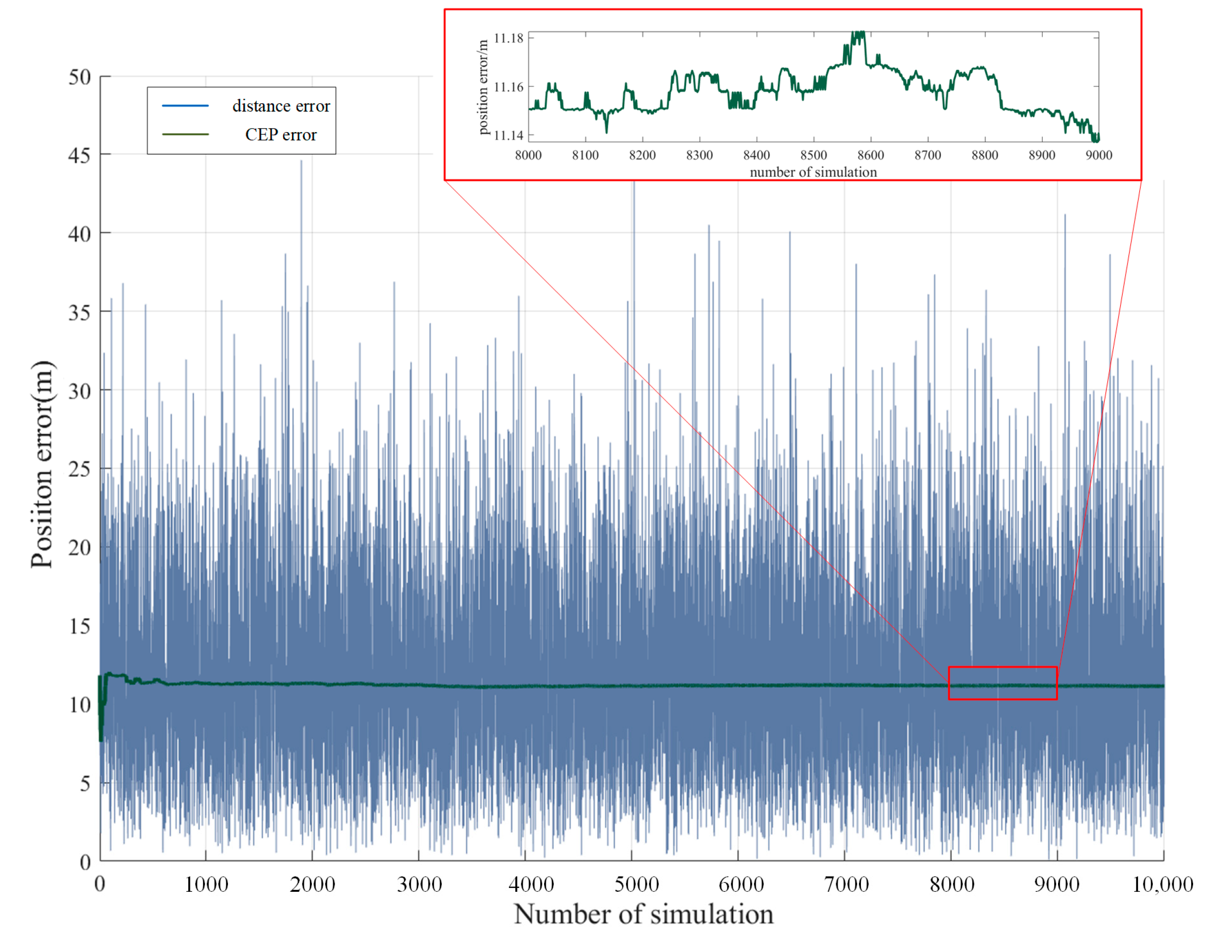
The ground in the simulation area is flat, so the positioning error caused by terrain fluctuation is temporarily not considered. During the simulation, the area with the center (31.20°N, 121.48°E) is photographed to obtain images by the UAV with a 2500 flight height. As shown in Figure 7, due to random error, the distance error simulation results in a single target location varying greatly, while the CEP gradually becomes stable when the simulation times exceed 1000, which can predict the positioning accuracy in the actual situation. Under the simulation conditions in 
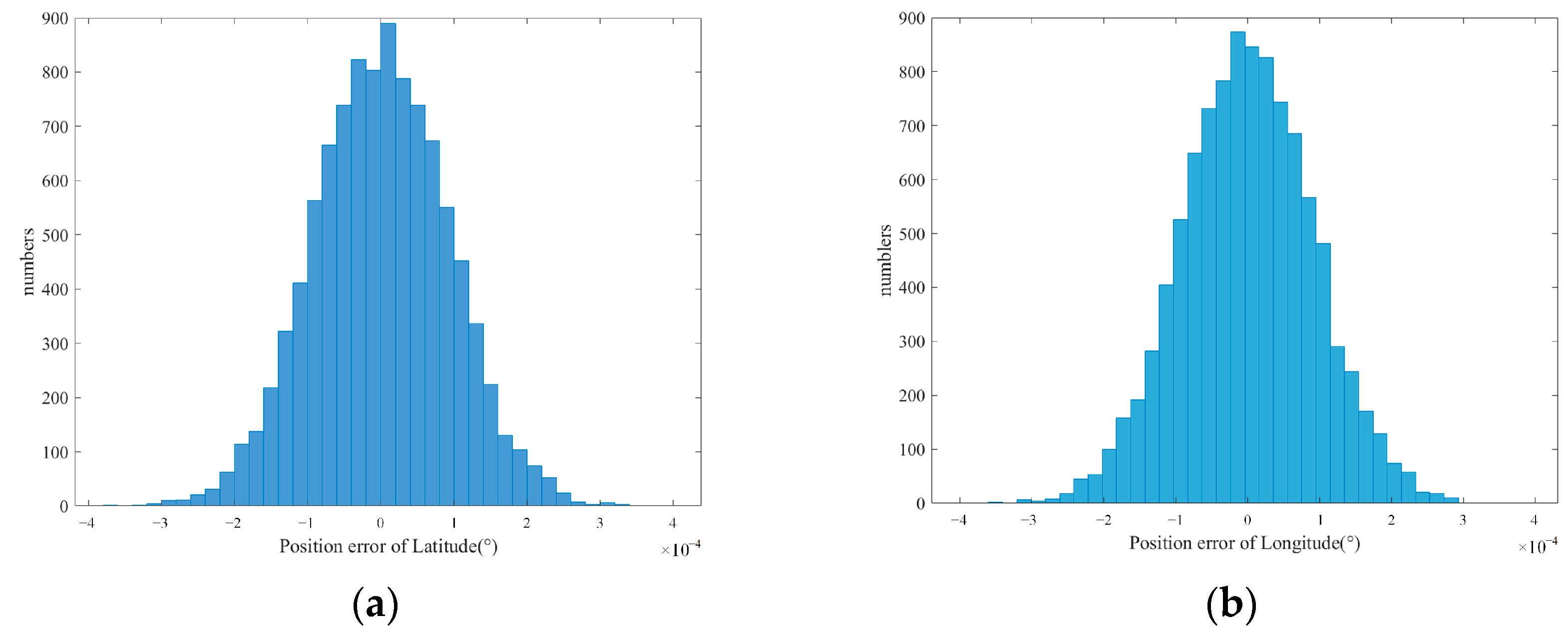
Table 1, the CEP is stable at around 11.15m, the projection position of the point to be registered in the image is a two-dimensional coordinate, and the pixel error during registration is also a two-dimensional parameter; therefore, considering their longitude and latitude errors separately is feasiable, and the registration error can be analyzed in combination with the longitude and latitude resolution of a single pixel. The longitude and latitude error probability distribution of aerial remote sensing images is shown in Figure 8.
The standard deviation of longitude and latitude of the simulation results can be calculated from the target reference position ( φ r , λ r ) and the positioning simulation result ( φ s , λ s ) , as shown in Equation (31).
σ φ = i = 1 N ( φ s φ r ) 2 N , σ λ = i = 1 N ( λ s λ r ) 2 N
Through calculation, the latitude standard deviation σ φ and longitude standard deviation σ λ are 0.0000937 ° and 0.0000923 ° , respectively. In addition, the pixel registration standard deviation of the point to be registered can be obtained by combining the longitude and latitude resolution calculated by Equation (21).
Similar to the calculation approach to data in Table 1, this paper simulated and analyzed the positioning accuracy of satellite remote sensing images through the data in Table 2. Figure 9 and Figure 10 illustrate the positioning error results.
Under the simulation parameters in Table 2, the latitude standard deviation of pixel positioning error σ φ is 0.000124 ° , and the longitude standard deviation σ λ is 0.000146 . Through analysis, it can be found that the CEP of satellite simulation positioning is 81.12 m, which is significantly higher than the simulation results of aerial remote sensing images. This is because a high earth orbit satellite is used to image the ground in the simulation process, which is more affected by various random errors such as attitude control, orbit measurement and position measurement than that of the low earth orbit satellite and UAVs. However, the positioning error does not mean that the registration accuracy will be reduced, since the specific pixel registration accuracy is limited by the pixel resolution, and the image resolution of the high earth orbit satellite is lower than that of the low-altitude UAV.
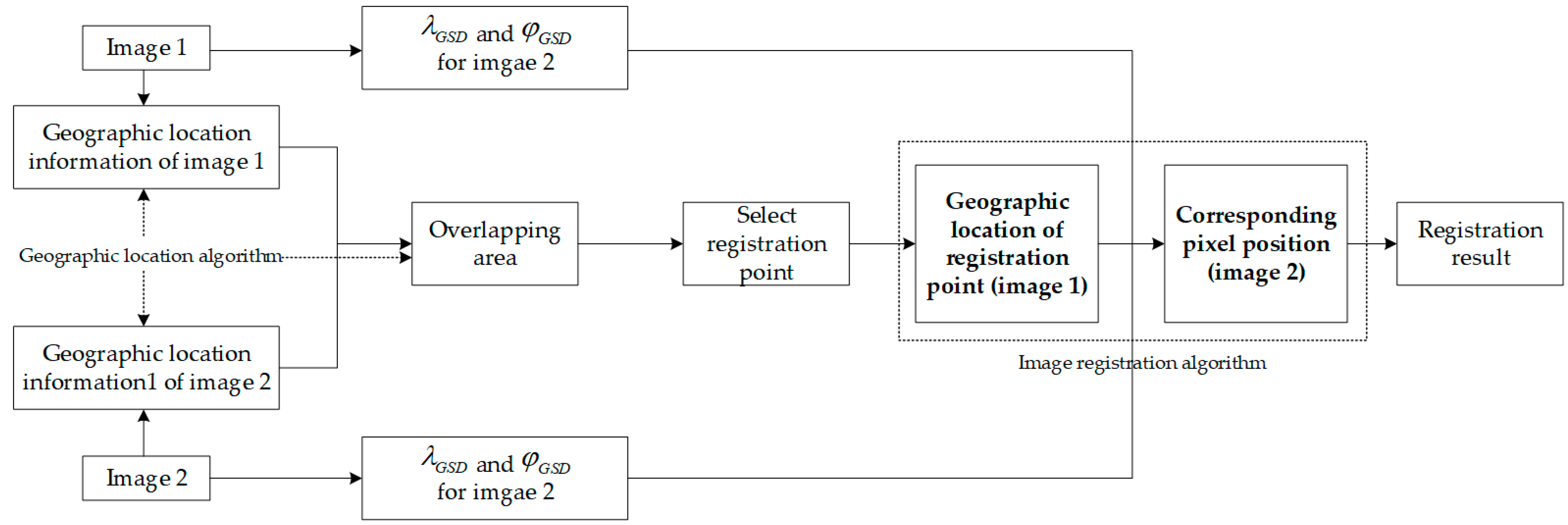
To verify the validity of this algorithm, the image registration process is simulated and analyzed through the simulation environment. Assuming that the area to be registered is within the range of 43.73 ° N 43.76 ° N , 125.36 ° E 125.40 ° E , Table 3 shows the geographic location information of the points selected for registration in the simulation. In the simulation process, the algorithms provided in Section 2 and Section 3 are used to calculate the geographic location and perform image registration. The simulation parameters are as follows: the pixel size of the UAV camera is 10 microns and the camera focal length is 0.06m. The camera CCD detector size is 2000 × 2000, and the carrier flight height is 3000 m. Under this simulation condition, the standard deviation of longitude positioning σ φ is 0.00016 ° , and the standard deviation of latitude positioning σ λ is 0.00011 ° .
The image to be registered is the satellite remote sensing image of the same area, the number of detector pixels is 4000 × 4000, the longitude positioning standard deviation σ φ is 0.00022 ° , and the latitude positioning standard deviation σ λ is 0.00015 ° . The distribution of pixel position calculation results of multiple simulation registration points is shown in Figure 11.
To display the simulation results more clearly and intuitively, the positioning error, projection error and registration point error are specifically analyzed, as shown in Table 4.
The projection error in the table refers to the pixel deviation distance between the projection position obtained by the coordinate transformation of the point to be registered and the actual projection position. However, due to random errors, the deviation directions of the points to be registered in the two images are not consistent. Therefore, the deviation between the actual projection position and the ideal projection position of the points to be registered should be considered; that is, the relative projection error of the points between the two images, which is recorded as the registration point error in the table. The ground registration accuracy can be calculated based on the ground resolution of the satellite image pixel of 0.5 m.
In the simulation experiment, all the data in Figure 11 are analyzed. The average projection errors of the three registration points on the two images are 34.53 pixels and 37.98 pixels, respectively. The average error of the relative registration points between the two images is 12.64 pixels, and the registration accuracy of the corresponding ground registration points is better than 6.5 m. This confirms that the algorithm can achieve image registration for the same area.

4.2. Registration Experiment of UAV Remote Sensing Image and Satellite Remote Sensing Image

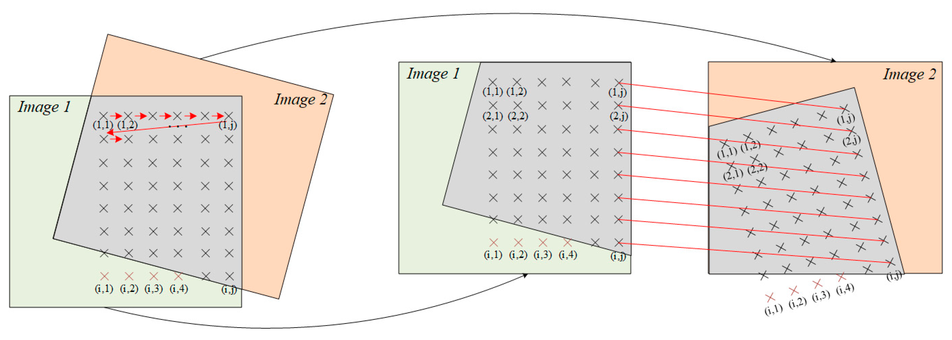
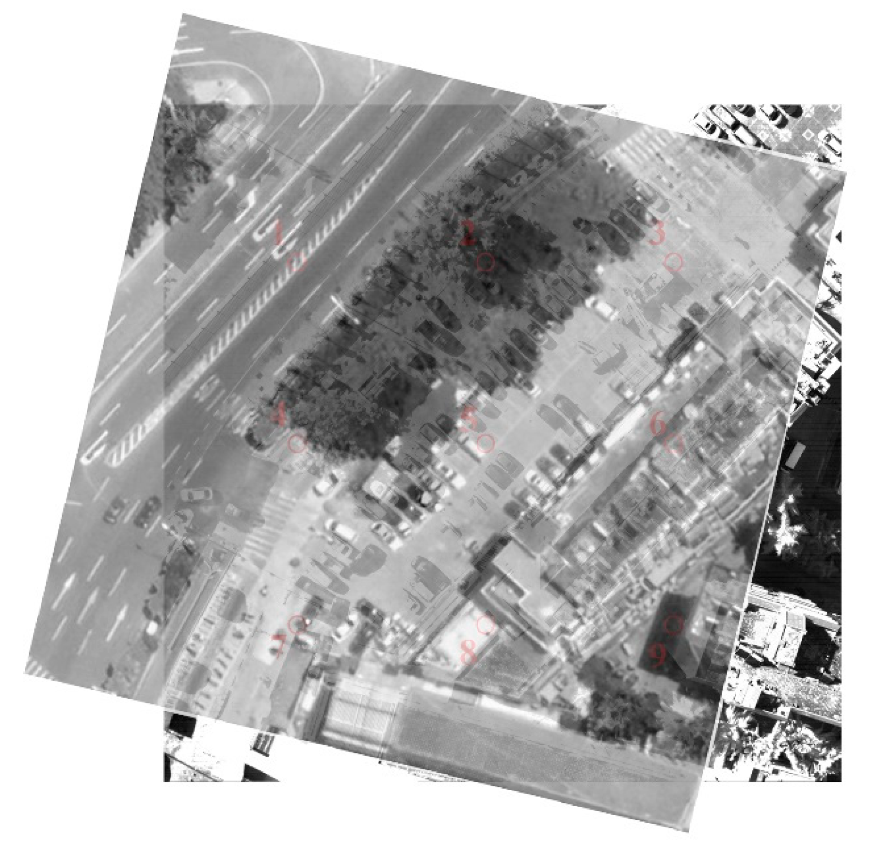
To verify the effectiveness of the geographic-information-based registration algorithm in the case of heterogeneous image registration, an aerial remote sensing image and satellite remote sensing image in the same area were randomly selected for registration experiments. However, the imaging angles and imaging time between the two images are different, and the coverage area is not completely consistent. The two images were obtained by high-resolution remote sensing satellites and ground remote sensing image obtained by UAVs, respectively. The resolution of the satellite remote sensing images is 0.15 m, and the ground resolution of UAV remote sensing images is 0.6 m. To better reflect the selection of registration points and the registration effect, the images are scaled in the schematic diagram to a uniform resolution.
First, two images were registered using the algorithm proposed in this paper. Nine groups of registration points were selected in the images, and the two images were registered by the algorithm proposed in Section 2 and Section 3. The corresponding positioning results and registration errors are recorded in Table 5. The geographic location information in the table was calculated according to the satellite remote sensing images to be registered. The projection position (UAV) is the ideal projection position of the point to be registered in the UAV remote sensing image calculated by the above algorithm. The registration error refers to the pixel deviation between the ideal position and the actual projection position. The registration accuracy can be represented by the spatial distance between the pixel position calculated by the algorithm and the standard position of the point to be registered.
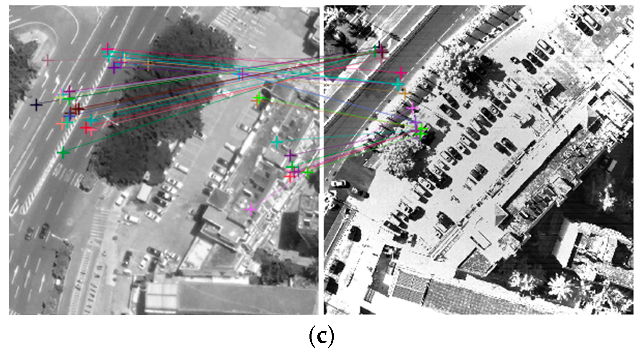
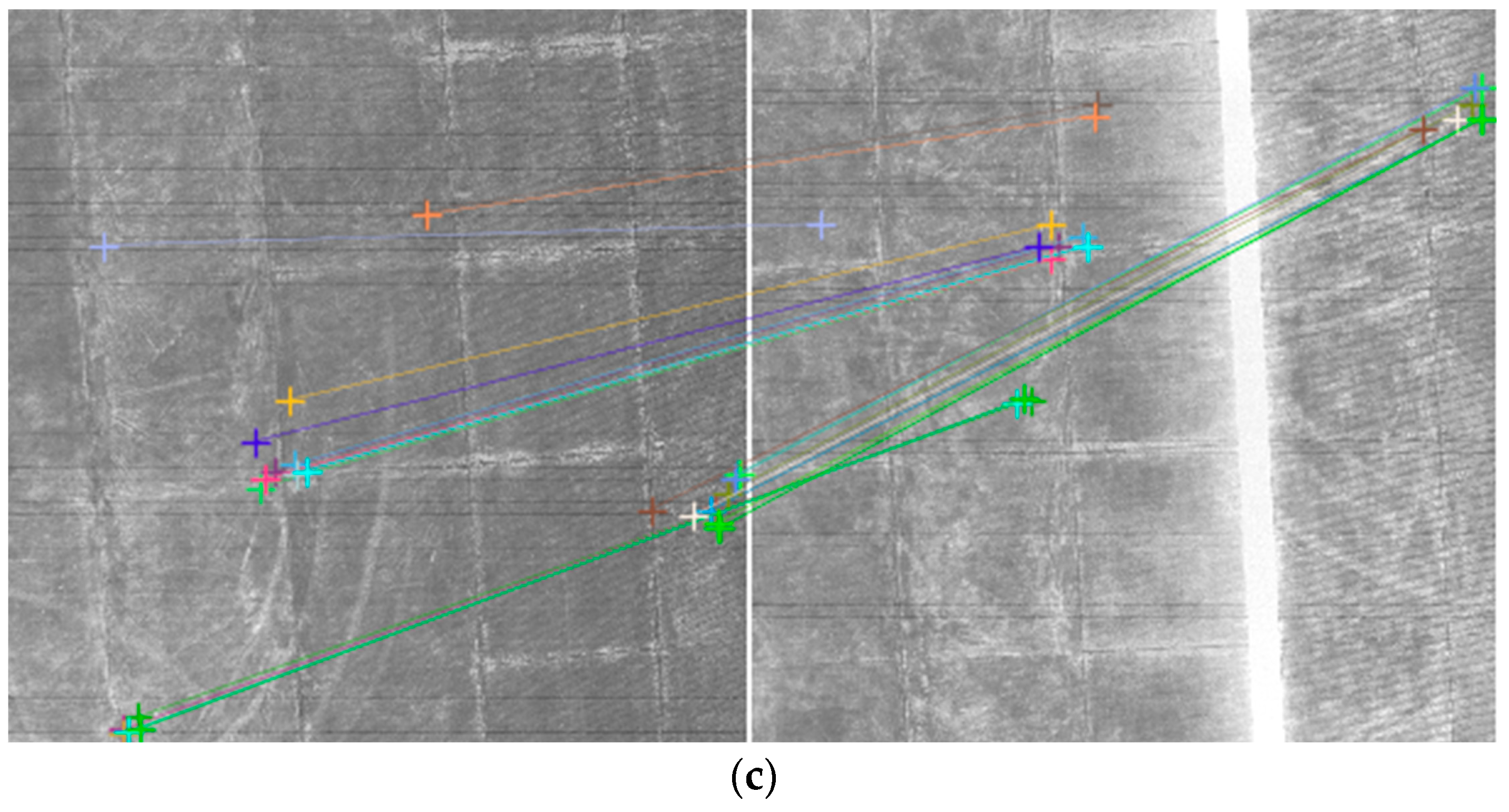
The experimental results show that GLI algorithm can register two images, the accuracy of ground registration reaches 12.55 m, and the exact correspondence between the two images can be obtained. Moreover, to verify the advantages of this algorithm in the case of heterologous image registration, SIFT-algorithm- and neural-network-based registration algorithms were used to register the two images in the experiment, and the results were compared with the GLI algorithm, as shown in Figure 12. The number in Figure 12a represents the selection order of registration points in the GLI algorithm, and the cross symbol in Figure 12c represents the position of feature points extracted by CNN.
To display the registration results more clearly, the experimental data were analyzed through the parameters of the number of registration points, the number of correctly matched pixels, and the average registration pixel error, as shown in Table 6. In the experiment, the SIFT algorithm obtained three groups of registration points, but all of them belonged to the wrong registration and the average registration error was 751.35 pixels. Many registration points were obtained by the neural network, of which only four groups were close to the correct registration and belonged to the same feature area, and the overall average registration error was 381.25 pixels. Neither method can give the corresponding relationship between the two images because there are too many misregistration points. The reason for this is that the two algorithms are based on image features, while the image to be registered has huge differences due to inconsistent shooting angles, changes in road signs, and changes in parking lot location and the number of vehicles. The number of wrong registrations is far greater than that of correct registrations. Therefore, the two algorithms cannot achieve image registration. Correspondingly, the GLI algorithm achieves image registration using the geographic location of nine sets of registration points, without considering image characteristics. Due to the positioning error, the average pixel error between the points to be registered was approximate 20.92 pixels. To verify the effectiveness of this algorithm, the registration errors of the image centers were also analyzed in Table 6. The data given in the table are the results of the calculation after the significant error registration points were manually removed. Since there are no correct registration points, SIFT cannot obtain registration results, and the average registration error of the neural network is 102.35 pixels.
The results show that the registration accuracy of the GLI algorithm is significantly better than that of the other two algorithms. When the feature-based registration algorithm struggles, the GLI algorithm can effectively register heterogeneous images with large differences. The final image registration result of this algorithm is shown in Figure 13.

4.3. Experiment with Image Registration without Feature Points

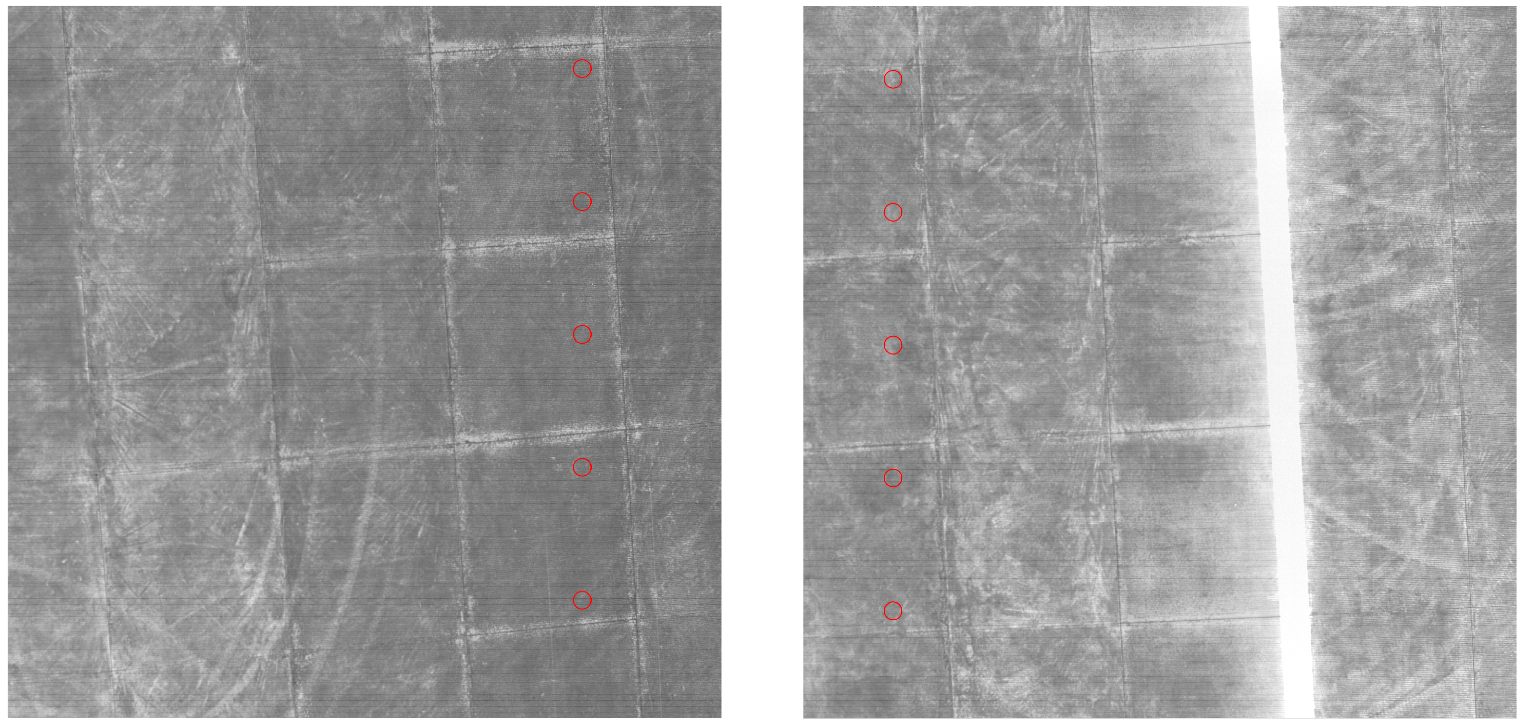
In the case where there are no obvious feature points, such as forest, farmland and sea level, the traditional registration algorithms cannot perform very well. Neither the SIFT algorithm nor the neural network model can find accurate matching feature points. In this paper, the registration ability of the GLI algorithm in the case of no feature points is verified by two consecutive farmland images taken by UAV.
Figure 14 shows two random remote sensing images of continuous farmland in the test area, with a certain area of overlap. After determining the overlapping area by calculating the geographic location corresponding to the pixel, five registration points are uniformly selected in the figure for the registration experiment and marked with a red circle, and the calculation results are shown in Table 7.
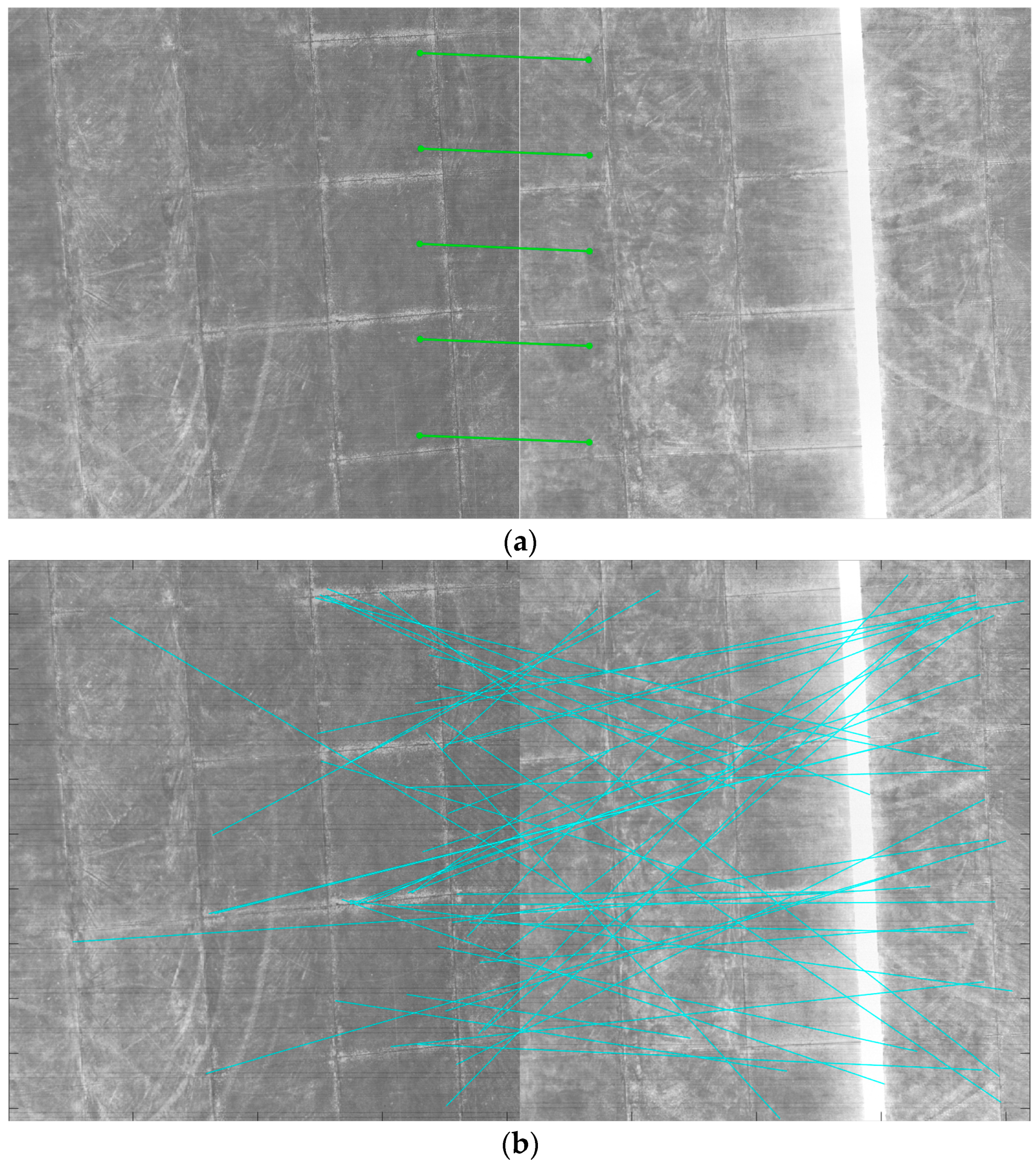
Figure 15 illustrates the registration results of the GLI algorithm, SIFT and CNN registration algorithm. As shown in the figure, since there are no typical feature points in the image, the algorithm based on feature extraction struggles to register two images. Both the SIFT algorithm and the neural network model extract the wrong registration points.
Similar to the experiment conducted in Section 4.2, the research in this section also takes registration points and registration accuracy as analysis criteria for experiment results. Since there are no typical features, such as geometric shape, in the farmland area, the registration results generated by SIFT algorithm are confusing and only one pair of registration points belongs to the same area of two images; however, this pair of registration points’ accuracy also reaches 245.62 pixels and the average registration error is 362.96 pixels. The neural network model partially recognized similar texture features but the extracted registration points do not belong to the same region. Therefore, the corresponding relationship between the two images cannot be derived. It should be noted that the average registration error does not reflect the real registration results because most of the registration points have the wrong registration and exceed the overlap region of the images. These registration errors, which have various directions in the coordinate system, mean that the comparison of average registration errors does not make much sense. Under this circumstance, the distribution of the quantity of correct and incorrect registrations ought to be more focused. As indicated in Table 8, the registration accuracy for SIFT is 2.17%, while the proportion is 0% for CNN-extracted feature point registration results. This phenomenon is caused by the uniform distribution of remote image texture, making the features of images from different regions very similar. This is also one of the reasons why the imaging registration algorithm based on feature points is difficult to apply to this kind of remote image.
For the GLI algorithm, the five groups of registration points obtained based on their geographical location information all have the correct registration, since the two images were continuously obtained by the same camera within a short time, and their positioning errors are also close. Therefore, the registration accuracy is only affected by the random measurement error during shooting. In this experiment, the pixel registration error is close to 7.2 pixels and the corresponding ground registration accuracy reaches 4.32 m, which can better achieve image registration without feature points.

5. Discussion

Simulation analysis and experiments indicate that the proposed algorithm, which is based on geographical location information, can achieve remote sensing image registration in the same region. This method does not involve the image features effect and only relies on the geographical location for registration. The registration accuracy is completely determined by the geographical location information of the image. In other words, it can be concluded that the registration accuracy of the algorithm is mainly affected by the following factors:
The precision of image photogrammetric information. The key to image registration through pixel location calculation is the geographic positioning accuracy of the algorithm, which is mainly affected by the measurement accuracy of photogrammetric parameters, such as imaging angle, position and attitude, satellite speed, UAV speed–height ratio, etc.
Positioning error caused by geometric deformation of the image. Besides the accuracy of angle measurement, image distortion is also one of the key factors affecting the results of pixel geographical location calculation. In practical tasks, there are a large number of images without geometric correction that need image registration. In this case, the position information in the image will deviate from the ideal position, which will lead to registration errors.
The image carries the precision of geographic information. Some images to be registered may have auxiliary information with reference positions, so they can be registered directly through the reference positions. The final registration accuracy is only affected by the accuracy of the information itself and the image resolution.
It should be noted that registration accuracy is more affected by positioning accuracy when the method is used to deal with the problem of heterogeneous image registration. This is because the random measurement errors of the two images are not consistent, which may lead to position errors in the ECEF coordinate system showing opposite directions in the pixel geographical location calculation process, resulting in poor registration accuracy. In this case, the core direction of optimizing this method is to reduce the errors in geographical positioning technology and achieve higher-precision image registration.

6. Conclusions

This paper proposes an image registration algorithm based on geographical location information. The image registration is realized by calculating the same geographical location’s corresponding location of different pixels in two paired images. This method is effective in the registration of arbitrary images, without the limitation of image features and imaging platforms. The experiments introduced in this paper are based on a real remote image dataset. The comparison among GLI, SIFT and CNN validates the proposed algorithm’s effectiveness. In the registration experiment conducted on remote images taken by UAV and satellites, SIFT only extracted three pairs of incorrect feature points and failed in image registration. In contrast, the image center registration error of the GLI is merely 21.24 pixels, which means that its accuracy compared to the CNN model improved by 85.08%. In the registration experiment regarding featureless and only partially overlapping remote sensing images, the CNN model failed to extract the right registration point; similarly, the registration accuracy of SIFT is as low as 2.17%. Through SIFT, the unique, successfully registered feature points’ pair error reaches 245.62 pixels. However, GLI’s accuracy is 100% because it can calculate the range of overlapping areas. Furthermore, GLI’s correct registration level is more optimal than 7.5 pixels, making it reliable for the real application of featureless image registration.
As the algorithm propounded in this paper calculates the geographical position of the registration region and pixel through imaging geometric relations, the registration effect entirely depends on the accuracy of the calculation. A practical means of ensuring the stability of the algorithm and improve the registration accuracy is continual research focusing on optimizing the geographical location calculation model in the future. For instance, distortion process flow can be added to the algorithm model so that the influence of geometric deformation is reduced. Moreover, the location error caused by environmental factors such as atmospheric refraction or topographic relief should also be considered in the location calculation and registration model to further improve the registration accuracy of heterogeneous images. The measurement precision of various sensors will also affect the registration accuracy of this algorithm, especially the precision level of the attitude and imaging angle.

Author Contributions

Conceptualization, X.Z. and Y.C.; methodology, X.Z. and Y.Z.; software, X.Z. and X.L.; validation J.L.; data curation, P.Q.; writing—original draft preparation, X.Z.; writing—review and editing, Y.C. and T.D. All authors have read and agreed to the published version of the manuscript.

Funding

This research received no external funding.

Data Availability Statement

Not applicable.

Conflicts of Interest

The authors declare no conflict of interest.

References

  1. Ye, Y.; Shan, J. A local descriptor based registration method for multispectral remote sensing images with non-linear intensity differences. ISPRS J. Photogramm. Remote Sens. 2014, 90, 83–95. [Google Scholar] [CrossRef]
  2. Misra, I.; Rohil, M.K.; Moorthi, M.; Dhar, D. Feature based remote sensing image registration techniques: A comprehensive and comparative review. Int. J. Remote Sens. 2022, 43, 4477–4516. [Google Scholar] [CrossRef]
  3. Wu, S.; Zhong, R.; Li, Q.; Qiao, K.; Zhu, Q. An Interband Registration Method for Hyperspectral Images Based on Adaptive Iterative Clustering. Remote Sens. 2021, 13, 1491. [Google Scholar] [CrossRef]
  4. Anuta, P.E. Digital Registration of Multispectral Video Imagery. Opt. Eng. 1969, 7, 706168. [Google Scholar] [CrossRef]
  5. Barnea, D.I.; Silverman, H.F. A class of algorithms for fast digital image registration. IEEE Trans. Comput. 1972, 100, 179–186. [Google Scholar] [CrossRef]
  6. Bajcs, R.; Kovacic, S. Multiresolution Elastic Matching. Comput. Vis. Graph. Image Process. 1989, 46, 1–21. [Google Scholar] [CrossRef]
  7. Roche, A.; Malandain, G.; Pennec, X.; Ayache, N. The correlation ratio as a new similarity measure for multimodal image registration. In Medical Image Computing and Computer-Assisted Intervention—MICCAI; Springer: Cambridge, MA, USA, 1998; pp. 1115–1124. [Google Scholar]
  8. Maes, F.; Collignon, A.; Vandermeulen, D.; Marchal, G.; Suetens, P. Multimodality image registration by maximization of mutual information. IEEE Trans. Med. Imaging 1997, 16, 187–198. [Google Scholar] [CrossRef] [Green Version]
  9. Liang, J.Y.; Liu, X.P.; Huang, K.N.; Li, X.; Wang, D.; Wang, X. Automatic registration of multisensor images using an integrated spatial and mutual information (SMI) metric. IEEE Trans. Geosci. Remote Sens. 2014, 52, 603–615. [Google Scholar] [CrossRef]
  10. Lowe, D.G. Distinctive Image Features from Scale-Invariant Keypoints. Int. J. Comput. Vis. 2004, 60, 91–110. [Google Scholar] [CrossRef]
  11. Sedaghat, A.; Mokhtarzade, M.; Ebadi, H. Uniform Robust Scale-Invariant Feature Matching for Optical Remote Sensing Images. IEEE Trans. Geosci. Remote Sens. 2011, 49, 4516–4527. [Google Scholar] [CrossRef]
  12. Paul, S.; Pati, U.C. Remote Sensing Optical Image Registration Using Modified Uniform Robust SIFT. IEEE Geosci. Remote Sens. Lett. 2016, 13, 1300–1304. [Google Scholar] [CrossRef]
  13. Yang, H.; Li, X.; Zhao, L.; Chen, S. A Novel Coarse-to-Fine Scheme for Remote Sensing Image Registration Based on SIFT and Phase Correlation. Remote Sens. 2019, 11, 1833. [Google Scholar] [CrossRef] [Green Version]
  14. Gong, X.; Yao, F.; Ma, J.; Jiang, J.; Lu, T.; Zhang, Y.; Zhou, H. Feature Matching for Remote-Sensing Image Registration via Neighborhood Topological and Affine Consistency. Remote Sens. 2022, 14, 2606. [Google Scholar] [CrossRef]
  15. Bay, H.; Tuytelaars, T.; Gool, L.V. SURF: Speeded up robust features. In Proceedings of the European Conference on Computer Vision, Graz, Austria, 7–13 May 2006; pp. 404–417. [Google Scholar]
  16. Dellinger, F.; Delon, J.; Gousseau, Y.; Michel, J. SAR-SIFT: A SIFT-Like Algorithm for SAR Images. IEEE Trans. Geosci. Remote Sens. 2015, 53, 453–466. [Google Scholar] [CrossRef] [Green Version]
  17. Sedaghat, A.; Ebadi, H. Remote Sensing Image Matching Based on Adaptive Binning SIFT Descriptor. IEEE Trans. Geosci. Remote Sens. 2015, 53, 5283–5293. [Google Scholar] [CrossRef]
  18. Liu, F.; Bi, F.; Chen, L.; Shi, H. Feature-Area Optimization: A Novel SAR Image Registration Method. IEEE Geosci. Remote Sens. Lett. 2016, 13, 242–246. [Google Scholar] [CrossRef] [Green Version]
  19. Ma, L.; Liu, Y.; Zhang, X.; Ye, Y.; Yin, G.; Johnson, B.A. Deep learning in remote sensing applications: A meta-analysis and review. ISPRS J. Photogramm. Remote Sens. 2019, 152, 166–177. [Google Scholar] [CrossRef]
  20. Li, L.; Han, L.; Ye, Y. Self-Supervised Keypoint Detection and Cross-Fusion Matching Networks for Multimodal Remote Sensing Image Registration. Remote Sens. 2022, 14, 3599. [Google Scholar] [CrossRef]
  21. Wang, S.; Quan, D.; Liang, X.; Ning, M.; Guo, Y.; Jiao, L. A deep learning framework for remote sensing image registration. ISPRS J. Photogramm. Remote Sens. 2018, 145, 148–164. [Google Scholar] [CrossRef]
  22. Maggiolo, L.; Solarna, D.; Moser, G.; Serpico, S.B. Registration of Multisensor Images through a Conditional Generative Adversarial Network and a Correlation-Type Similarity Measure. Remote Sens. 2022, 14, 2811. [Google Scholar] [CrossRef]
  23. Feng, R.; Li, X.; Bai, J.; Ye, Y. MID: A Novel Mountainous Remote Sensing Imagery Registration Dataset Assessed by a Coarse-to-Fine Unsupervised Cascading Network. Remote Sens. 2022, 14, 4178. [Google Scholar] [CrossRef]
  24. Driben, R.; Konotop, V.V.; Meier, T. Precession andnutation dynamics of nonlinearly coupled non-coaxial three-dimensional matter wave vortices. Sci. Rep. 2016, 6, 22758. [Google Scholar] [CrossRef] [Green Version]
  25. Zhang, F.; Xu, G.; Jean-Pierre, B. Keplerian orbit elements induced by precession, nutation and polar motion. Prog. Geophys. 2019, 34, 2205–2211. [Google Scholar]
  26. Zhang, L.; Zhang, X.; Yue, Q.; Liu, N.; Sun, K.; Sun, J.; Fan, G. Attitude Planning and Fast Simulation Method of Optical Remote Sensing Satellite Staring Imaging. J. Jilin Univ. (Eng. Ed.) 2021, 51, 340–348. [Google Scholar] [CrossRef]
  27. Ioannidou, S.; Pantazis, G. Helmert Transformation Problem. From Euler Angles Method to Quaternion Algebra. ISPRS Int. J. Geo-Inf. 2020, 9, 494. [Google Scholar] [CrossRef]
  28. Wang, G.; Liu, X.; Han, S. A Method of Robot Base Frame Calibration by Using Dual Quaternion Algebra. IEEE Access 2018, 6, 74865–74873. [Google Scholar] [CrossRef]
  29. Ossokine, S.; Kidder, L.E.; Pfeiffer, H.P. Precession-tracking coordinates for simulations of compact-object binaries. Phys. Rev. D 2013, 88, 084031. [Google Scholar] [CrossRef]
Figure 1. ECEF coordinate system and description of longitude and latitude.
Remotesensing 15 00436 g001
Figure 2. Coordinate system in satellite image geographic positioning.
Remotesensing 15 00436 g002
Figure 3. Coordinate system in airborne image geographic positioning.
Remotesensing 15 00436 g003
Figure 4. Selection of registration points for image coincidence area.
Remotesensing 15 00436 g004
Figure 5. Registration point selection process.
Remotesensing 15 00436 g005
Figure 6. Overall flow diagram of the algorithm.
Remotesensing 15 00436 g006
Figure 7. Analysis of geographical position error of aerial remote sensing image.
Remotesensing 15 00436 g007
Figure 8. Probability distribution of longitude and latitude error. (a) Latitude error distribution; (b) Longitude error distribution.
Remotesensing 15 00436 g008
Figure 9. Analysis of geographical position error of satellite remote sensing image.
Remotesensing 15 00436 g009
Figure 10. Probability distribution of longitude and latitude error. (a) Latitude error distribution; (b) longitude error distribution.
Remotesensing 15 00436 g010
Figure 11. Distribution of registration points on simulated images. (a) Calculation results of registration point 1 in aerial remote sensing image; (b) calculation results of registration point 1 in satellite remote sensing image; (c) calculation results of registration point 2 in aerial remote sensing image; (d) calculation results of registration point 2 in satellite remote sensing image; (e) calculation results of registration point 3 in aerial remote sensing image; (f) calculation results of registration point 3 in satellite remote sensing image.
Remotesensing 15 00436 g011
Figure 12. Experimental results of heterogeneous remote sensing image registration. (a) Image registration algorithm based on geographic location information; (b) image registration algorithm based on SIFT; (c) image registration algorithm based on neural network model.
Remotesensing 15 00436 g012aRemotesensing 15 00436 g012b
Figure 13. Effect of heterogeneous image registration.
Remotesensing 15 00436 g013
Figure 14. Schematic diagram of feature free image and registration point selection.
Remotesensing 15 00436 g014
Figure 15. Experimental results of featureless remote sensing image registration. (a) Image registration algorithm based on geographic location information; (b) image registration algorithm based on SIFT; (c) image registration algorithm based on a neural network model.
Remotesensing 15 00436 g015aRemotesensing 15 00436 g015b
Table 1. Simulation parameters of aerial remote sensing images.
VariableReference ValueStandard DeviationUnit
ECEF coordinate (x)−2,852,931.4410m
ECEF coordinate (y)4,657,887.1210m
ECEF coordinate (z)3,287,036.4010m
Roll300.02°
Pitch150.02°
Yaw00.02°
θ p i t c h 0–300.005°
θ r o l l 0.50.005°
Table 2. Simulation parameters of satellite remote sensing images.
VariableReference ValueStandard DeviationUnit
J2000 coordinate (x)5,721,150.32100m
J2000 coordinate (y)3,817,990.65100m
J2000 coordinate (z)−12,360.1650m
Speed (x)−2,976.4510m/s
Speed (y)4,477.5810m/s
Speed (z)5,389.245m/s
Roll28.07550.0001°
Pitch42.15550.0001°
Yaw−5.812230.0001°
Pixel deviation caused by the temperature field(0,0)1pixel
Table 3. Parameters of registration points.
Registration Point123
longitude43.760843.745043.7429
latitude125.3752125.3957125.3820
height217.2217.6216.5
Table 4. Simulation data.
Registration PointNumber of SimulationsPositioning Error(A)Projection Error(S)Registration Point ErrorGround Registration Accuracy
11023.6626.28.94.45
20535.6839.615.27.60
48753.7825.916.48.20
76938.4359.713.56.75
213684.8236.718.89.40
55132.6622.84.72.35
39571.117.8414.37.15
84626.2742.53.91.95
323843.7626.82.71.35
33757.8955.316.78.35
56911.9713.63.21.60
92018.1058.910.75.35
Table 5. Experimental results of heterogenous image registration.
Registration PointLongitudeLatitudeProjection Position (UAV)Registration Error (Pixel)Registration Accuracy (m)
1109.515518.2339445.5, 487.221.112.67
2109.515818.2340989.3, 486.919.611.79
3109.516118.23411533.7, 487.821.112.71
4109.515618.2333446.3, 1006.222.713.63
5109.515818.2338988.7, 1005.320.812.48
6109.516118.23391532.9, 1006.421.713.03
7109.515718.2335445.8, 1525.121.212.72
8109.515918.2336989.6, 1526.219.411.69
9109.516118.23361532.6, 1524.920.412.29
Table 6. Comparative analysis of experimental results.
AlgorithmNumber of the Registration PointNumber of the Correct Registration PointAverage Registration Error (Pixels)Registration Error of Image Center (Pixels)
GLI9920.9221.24
SIFT30751.35N/A
CNN374381.25142.35
Table 7. Calculation results of geographical position of registered pixel points.
Registration PointProjection Position (a)LongitudeLatitudeProjection Position (b)Registration ErrorRegistration Accuracy (m)
11647,183109.515518.2339445.5,487.221.112.67
21647,565109.515818.2340989.3,486.919.611.79
31647,947109.516118.23411533.7,487.821.112.71
41647,1329109.515618.2333446.3,1006.222.713.63
51647,1711109.515818.2338988.7,1005.320.812.48
Table 8. Comparison of experiment results.
AlgorithmAverage Registration Error (Pixels)Number of Registration PointNumber of Correct Registration PointRegistration
Accuracy (m)
CLI7.4255100%
SIFT362.964612.17%
CNN271.972400%
Disclaimer/Publisher’s Note: The statements, opinions and data contained in all publications are solely those of the individual author(s) and contributor(s) and not of MDPI and/or the editor(s). MDPI and/or the editor(s) disclaim responsibility for any injury to people or property resulting from any ideas, methods, instructions or products referred to in the content.

