
A Novel Algorithm of Haze Identification Based on FY3D/MERSI-II Remote Sensing Data

 , ,
, ,  ,
,
Abstract
:1. Introduction
2. Materials and Methods
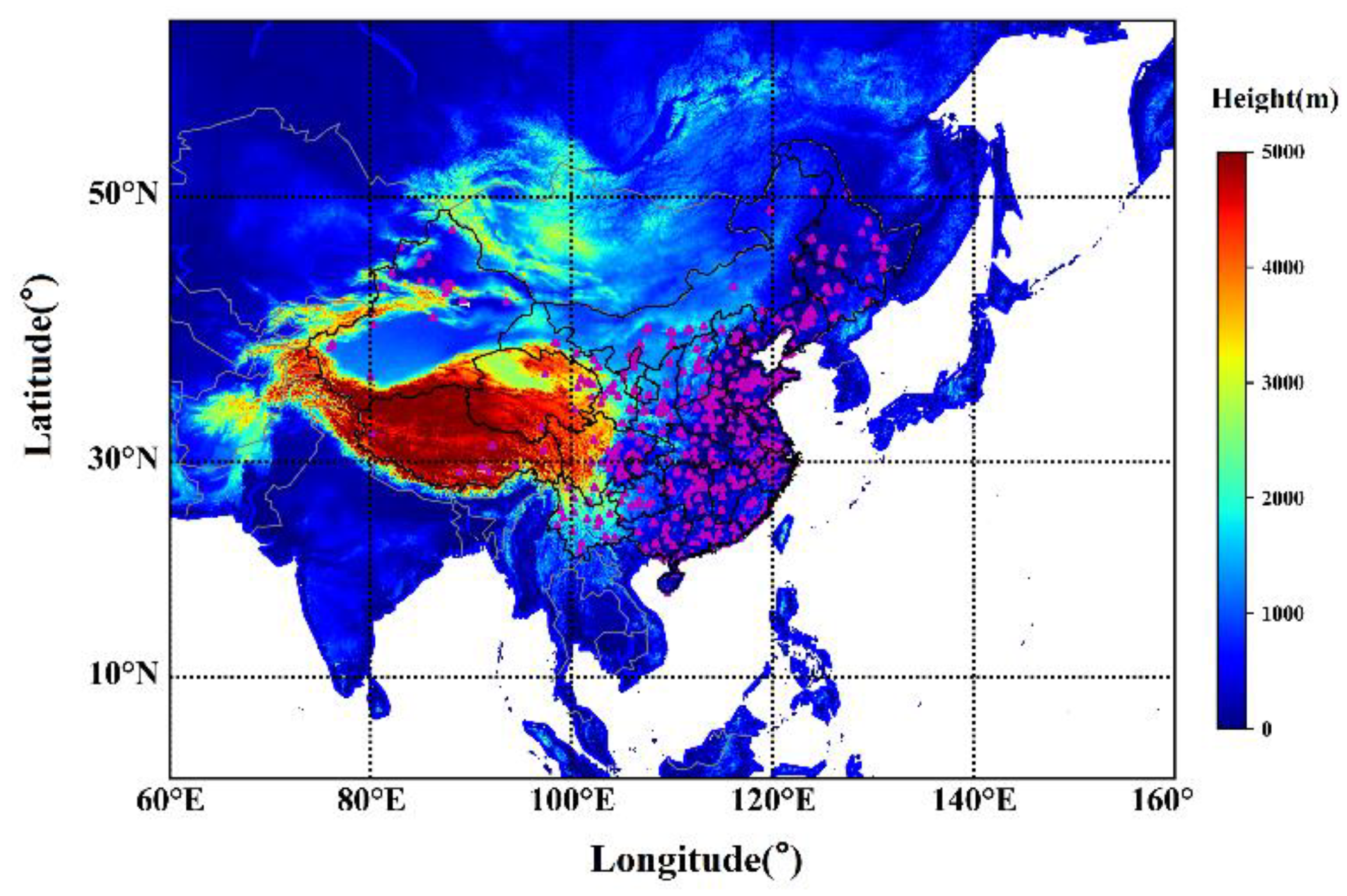
2.1. Study Domain
2.2. Data Sources
2.2.1. FY3D/MERSI-II
2.2.2. Aqua/MODIS
2.2.3. Auxiliary Datasets
2.3. MHAM Algorithm
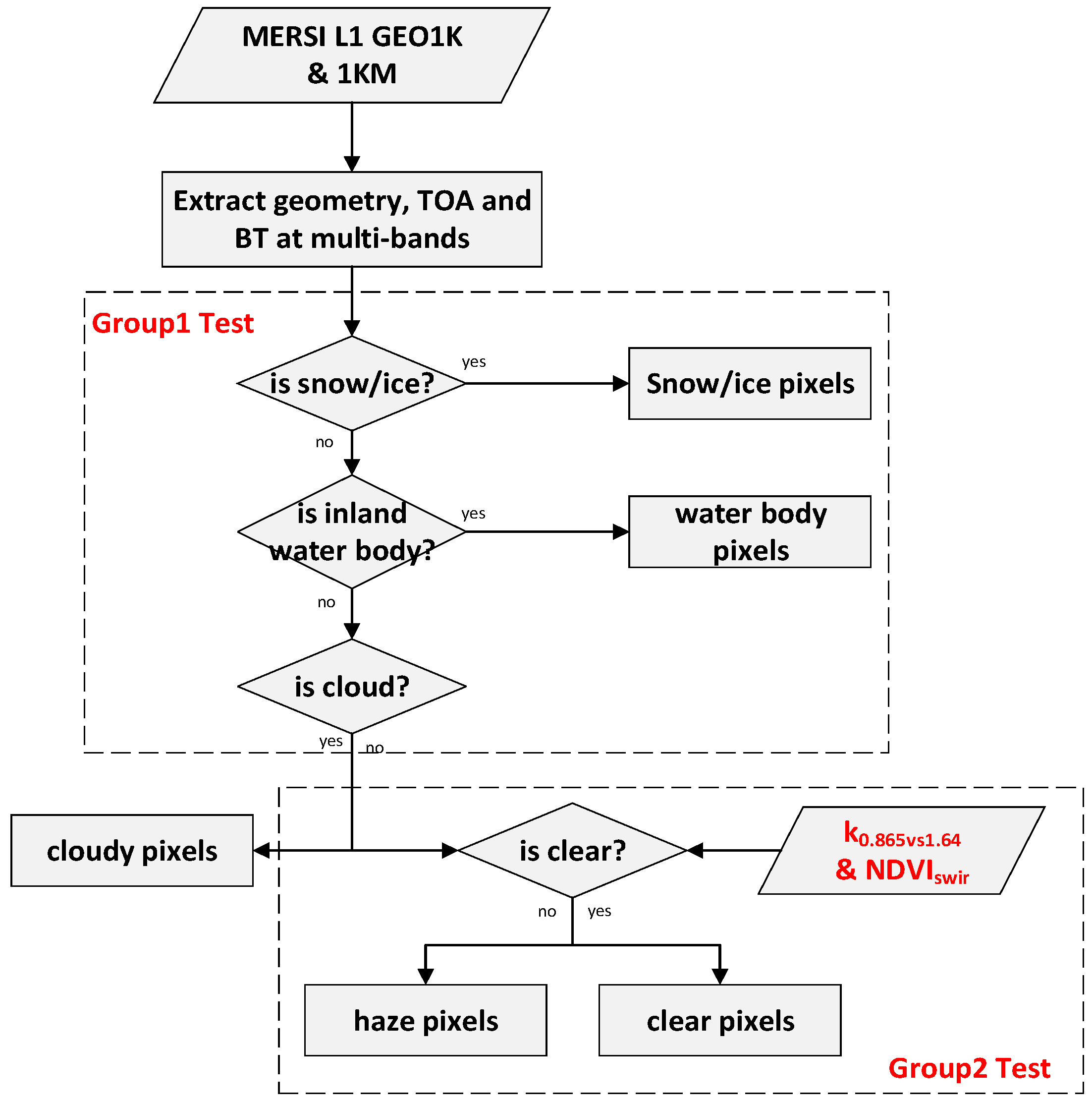
2.3.1. Algorithm Description
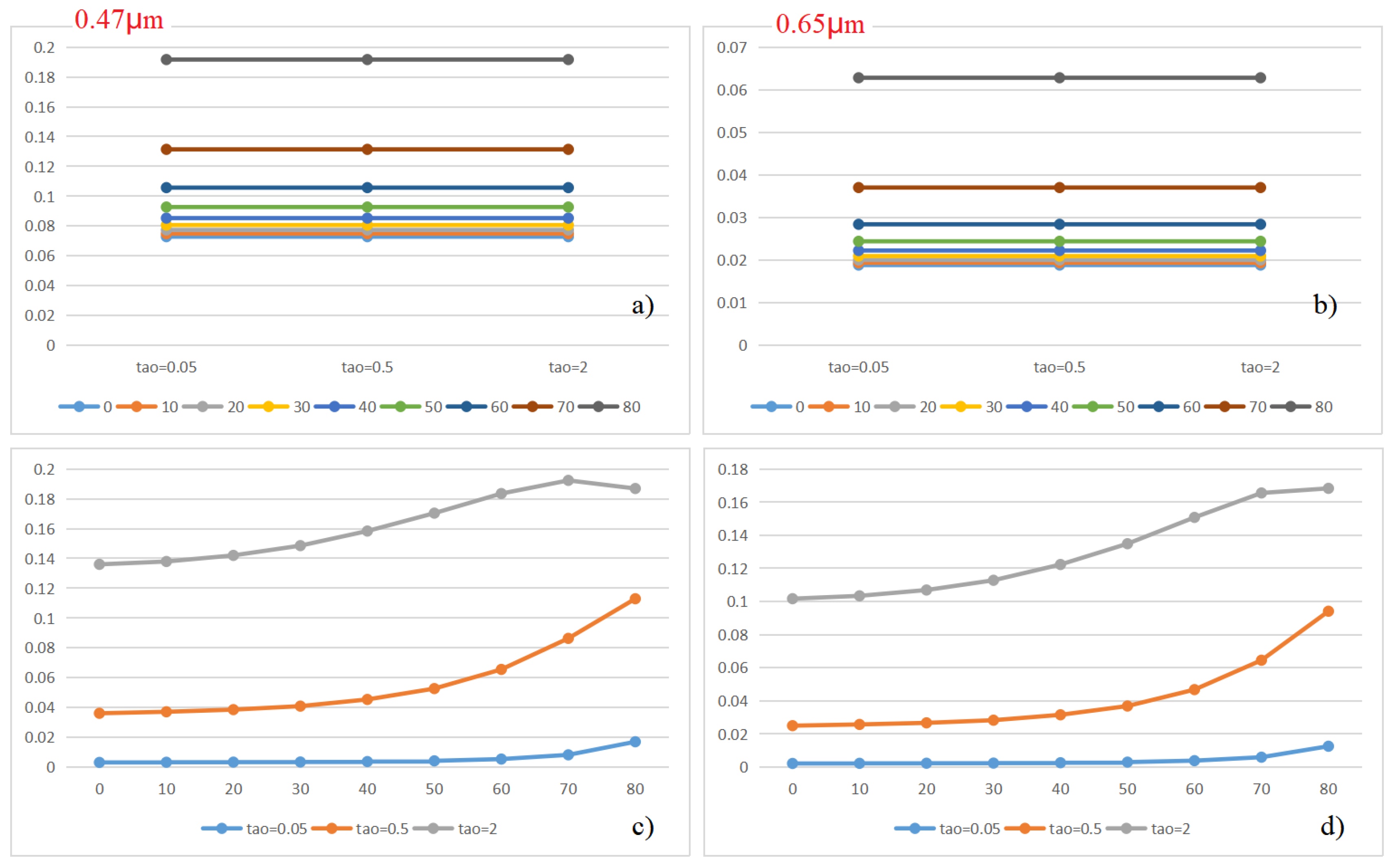
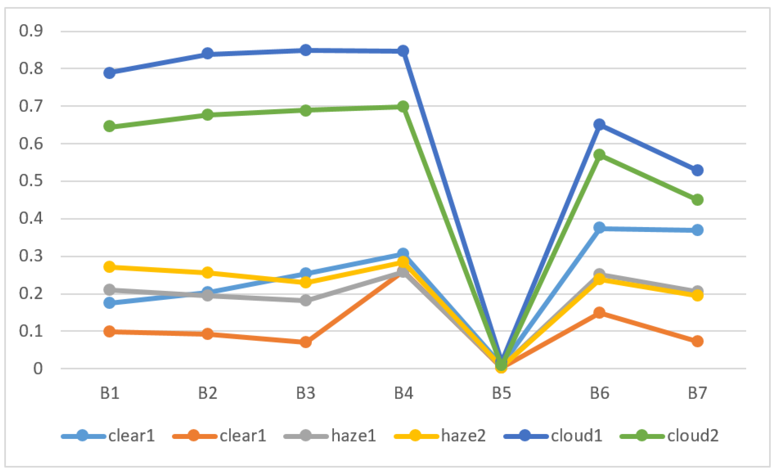
2.3.2. Selection of Spectral Characterization Based on FY3D/MERSI-II
2.3.3. Identification of Clear Conditions over Bright Surface
2.3.4. Single Threshold Tests
Cloud Threshold Tests
Clear Threshold Tests
3. Results
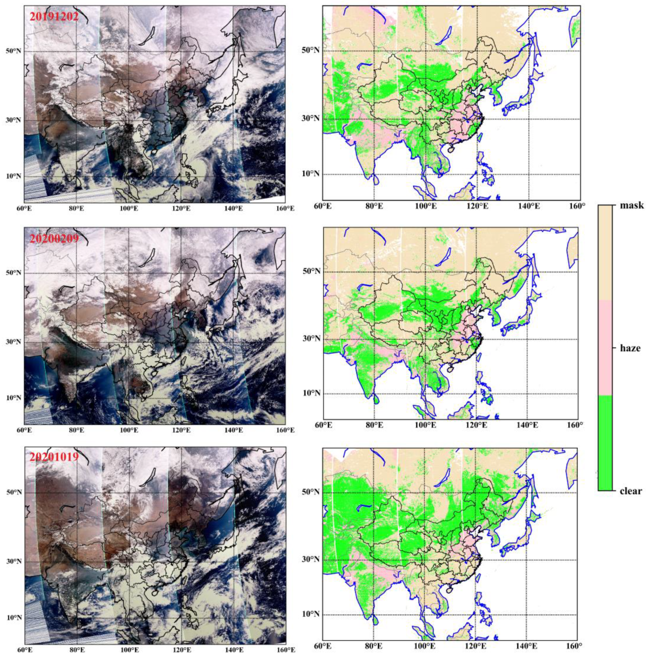
3.1. Distribution of Haze Identification
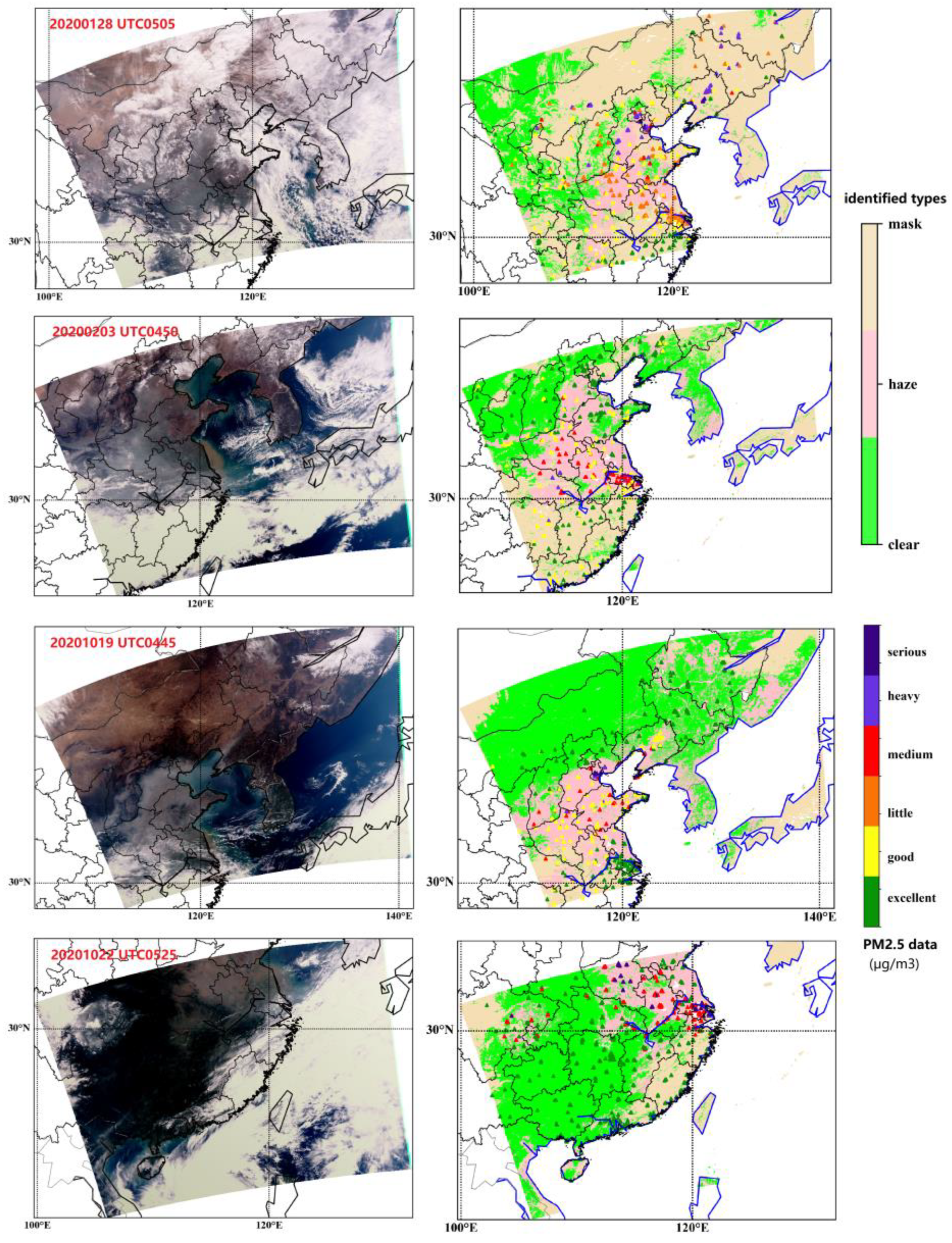
3.2. Validation against PM2.5 Measurements
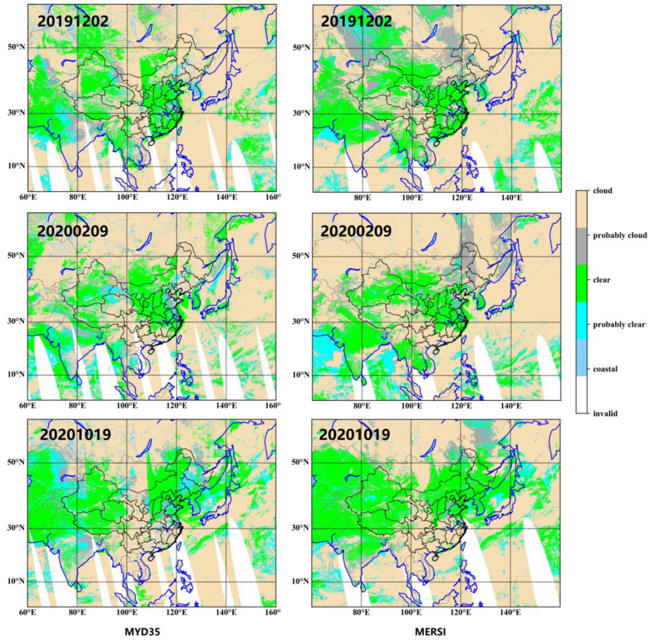
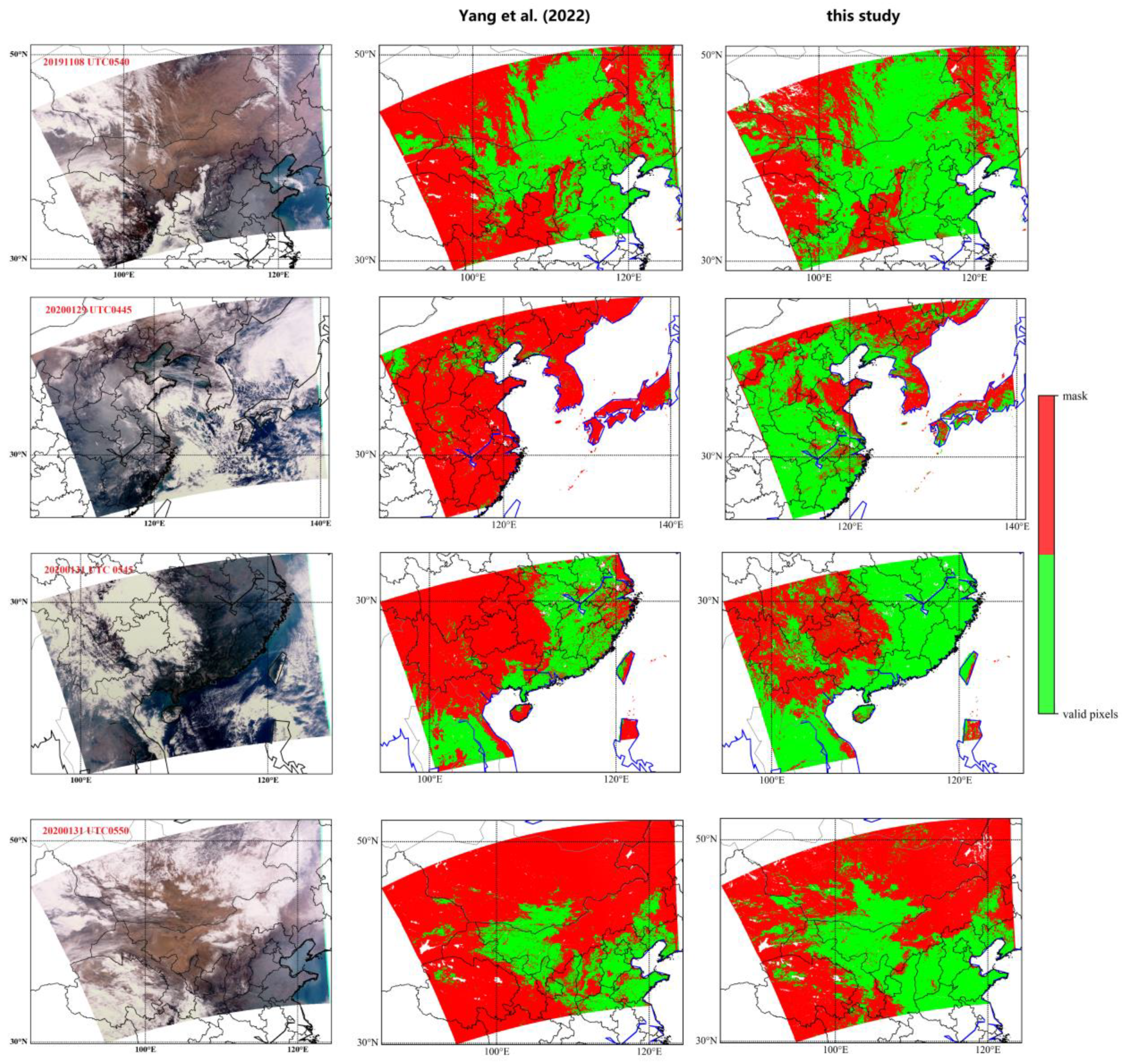
3.3. Cross-Comparison with Other Method
4. Conclusions
Author Contributions
Funding
Data Availability Statement
Acknowledgments
Conflicts of Interest
References
- Wu, D. A Discussion on Difference between Haze and Fog and Warning of Ash Haze Weather. Meteorol. Mon. 2005, 31, 7. [Google Scholar]
- Gautam, R.; Hsu, N.C.; Eck, T.F.; Holben, B.N.; Janjai, S.; Jantarach, T.; Tsay, S.C.; Lau, W.K. Characterization of aerosols over the Indochina peninsula from satellite-surface observations during biomass burning pre-monsoon season. Atmos. Environ. 2013, 78, 51–59. [Google Scholar] [CrossRef]
- Menon, S.; Hansen, J.; Nazarenko, L.; Luo, Y.F. Climate effects of black carbon aerosols in China and India. Science 2002, 297, 2250–2253. [Google Scholar] [CrossRef] [PubMed] [Green Version]
- Zhang, X.Y.; Wang, F.; Wang, W.H.; Huang, F.X.; Chen, B.L.; Gao, L.; Wang, S.P.; Yan, H.H.; Ye, H.H.; Si, F.Q.; et al. The development and application of satellite remote sensing for atmospheric compositions in China. Atmos. Res. 2020, 245, 105056. [Google Scholar] [CrossRef]
- Xia, X.A.; Chen, H.B.; Wang, P.C.; Zhang, W.X.; Goloub, P.; Chatenet, B.; Eck, T.F.; Holben, B.N. Variation of column-integrated aerosol properties in a Chinese urban region. J. Geophys. Res.-Atmos. 2006, 111. [Google Scholar] [CrossRef]
- Liu, X.G.; Li, J.; Qu, Y.; Han, T.; Hou, L.; Gu, J.; Chen, C.; Yang, Y.; Liu, X.; Yang, T.; et al. Formation and evolution mechanism of regional haze: A case study in the megacity Beijing, China. Atmos. Chem. Phys. 2013, 13, 4501–4514. [Google Scholar] [CrossRef] [Green Version]
- Zhang, X.; Wang, H.; Che, H.Z.; Tan, S.C.; Shi, G.Y.; Yao, X.P. The impact of aerosol on MODIS cloud detection and property retrieval in seriously polluted East China. Sci. Total Environ. 2020, 711, 134634. [Google Scholar] [CrossRef] [PubMed]
- Che, H.; Xia, X.; Zhu, J.; Li, Z.; Dubovik, O.; Holben, B.; Goloub, P.; Chen, H.; Estelles, V.; Cuevas-Agullo, E.; et al. Column aerosol optical properties and aerosol radiative forcing during a serious haze-fog month over North China Plain in 2013 based on ground-based sunphotometer measurements. Atmos. Chem. Phys. 2014, 14, 2125–2138. [Google Scholar] [CrossRef] [Green Version]
- Cheng, Z.; Wang, S.; Fu, X.; Watson, J.G.; Jiang, J.; Fu, Q.; Chen, C.; Xu, B.; Yu, J.; Chow, J.C.; et al. Impact of biomass burning on haze pollution in the Yangtze River delta, China: A case study in summer 2011. Atmos. Chem. Phys. 2014, 14, 4573–4585. [Google Scholar] [CrossRef] [Green Version]
- Tao, M.H.; Chen, L.F.; Wang, Z.F.; Wang, J.; Tao, J.H.; Wang, X.H. Did the widespread haze pollution over China increase during the last decade? A satellite view from space. Environ. Res. Lett. 2016, 11, 054019. [Google Scholar] [CrossRef]
- Tao, M.H.; Chen, L.F.; Xiong, X.Z.; Zhang, M.G.; Ma, P.F.; Tao, J.H.; Wang, Z.F. Formation process of the widespread extreme haze pollution over northern China in January 2013: Implications for regional air quality and climate. Atmos. Environ. 2014, 98, 417–425. [Google Scholar] [CrossRef]
- Tao, M.H.; Li, R.; Wang, L.L.; Lan, F.; Wang, Z.F.; Tao, J.H.; Che, H.Z.; Wang, L.C.; Chen, L.F. A critical view of long-term AVHRR aerosol data record in China: Retrieval frequency and heavy pollution. Atmos. Environ. 2020, 223, 117246. [Google Scholar] [CrossRef]
- Lim, H.; Choi, M.; Kim, J.; Kasai, Y.; Chan, P.W. AHI/Himawari-8 Yonsei Aerosol Retrieval (YAER): Algorithm, Validation and Merged Products. Remote Sens. 2018, 10, 699. [Google Scholar] [CrossRef] [Green Version]
- Remer, L.A.; Mattoo, S.; Levy, R.C.; Heidinger, A.; Pierce, R.B.; Chin, M. Retrieving aerosol in a cloudy environment: Aerosol product availability as a function of spatial resolution. Atmos. Meas. Tech. 2012, 5, 1823–1840. [Google Scholar] [CrossRef] [Green Version]
- Wang, Y.; Chen, L.F.; Li, S.S.; Wang, X.H.; Yu, C.; Si, Y.D.; Zhang, Z.L. Interference of Heavy Aerosol Loading on the VIIRS Aerosol Optical Depth (AOD) Retrieval Algorithm. Remote Sens. 2017, 9, 397. [Google Scholar] [CrossRef] [Green Version]
- Zeng, S.; Parol, F.; Riedi, J.; Cornet, C.; Thieuleux, F. Examination of POLDER/PARASOL and MODIS/Aqua Cloud Fractions and Properties Representativeness. J. Clim. 2011, 24, 4435–4450. [Google Scholar] [CrossRef]
- Levy, R.C.; Mattoo, S.; Munchak, L.A.; Remer, L.A.; Sayer, A.M.; Patadia, F.; Hsu, N.C. The Collection 6 MODIS aerosol products over land and ocean. Atmos. Meas. Tech. 2013, 6, 2989–3034. [Google Scholar] [CrossRef] [Green Version]
- Hutchison, K.D.; Iisager, B.D.; Kopp, T.J.; Jackson, J.M. Distinguishing aerosols from clouds in global, multispectral satellite data with automated cloud classification algorithms. J. Atmos. Ocean. Technol. 2008, 25, 501–518. [Google Scholar] [CrossRef]
- Ge, W.; Chen, L.F.; Si, Y.D.; Ge, Q.; Fan, M.; Li, S.S. Haze Spectral Analysis and Detection Algorithm Using Satellite Remote Sensing Data. Spectrosc. Spectr. Anal. 2016, 36, 3817–3824. [Google Scholar]
- Shang, H.Z.; Chen, L.F.; Tao, J.H.; Su, L.; Jia, S.L. Synergetic Use of MODIS Cloud Parameters for Distinguishing High Aerosol Loadings from Clouds Over the North China Plain. IEEE J. Sel. Top. Appl. Earth Obs. Remote Sens. 2014, 7, 4879–4886. [Google Scholar] [CrossRef]
- Ackerman, S.A.; Strabala, K.I.; Menzel, W.P.; Frey, R.A.; Moeller, C.C.; Gumley, L.E. Discriminating clear sky from clouds with MODIS. J. Geophys. Res.-Atmos. 1998, 103, 16. [Google Scholar] [CrossRef]
- Shang, H.Z.; Chen, L.F.; Letu, H.S.; Zhao, M.; Li, S.S.; Bao, S.H. Development of a daytime cloud and haze detection algorithm for Himawari-8 satellite measurements over central and eastern China. J. Geophys. Res.-Atmos. 2017, 122, 3528–3543. [Google Scholar] [CrossRef]
- Yang, L.K.; Hu, X.Q.; Wang, H.; He, X.W.; Liu, P.; Xu, N.; Yang, Z.D.; Zhang, P. Preliminary test of quantitative capability in aerosol retrieval over land from MERSI-II onboard FY3D. Natl. Remote Sens. Bull. 2022, 26, 923–940. [Google Scholar]
- Shi, Y.X.R.; Levy, R.C.; Yang, L.K.; Remer, L.A.; Mattoo, S.; Dubovik, O. A Dark Target research aerosol algorithm for MODIS observations over eastern China: Increasing coverage while maintaining accuracy at high aerosol loading. Atmos. Meas. Tech. 2021, 14, 3449–3468. [Google Scholar] [CrossRef]
- Yang, Z.D.; Lu, N.M.; Shi, J.M.; Zhang, P.; Dong, C.H.; Yang, J. Overview of FY-3 Payload and Ground Application System. IEEE Trans. Geosci. Remote Sens. 2012, 50, 4846–4853. [Google Scholar] [CrossRef]
- Hu, X.Q.; Liu, J.J.; Sun, L.; Rong, Z.G.; Li, Y.; Zhang, Y.; Zheng, Z.J.; Wu, R.H.; Zhang, L.J.; Gu, X.F. Characterization of CRCS Dunhuang test site and vicarious calibration utilization for Fengyun (FY) series sensors. Can. J. Remote Sens. 2010, 36, 566–582. [Google Scholar] [CrossRef]
- Hu, X.Q.; Sun, L.; Liu, J.J.; Ding, L.; Wang, X.H.; Li, Y.; Zhang, Y.; Xu, N.; Chen, L. Calibration for the Solar Reflective Bands of Medium Resolution Spectral Imager Onboard FY-3A. IEEE Trans. Geosci. Remote Sens. 2012, 50, 4915–4928. [Google Scholar] [CrossRef]
- Xu, N.; Niu, X.H.; Hu, X.Q.; Wang, X.H.; Wu, R.H.; Chen, S.S.; Chen, L.; Sun, L.; Ding, L.; Yang, Z.D.; et al. Prelaunch Calibration and Radiometric Performance of the Advanced MERSI II on FengYun-3D. IEEE Trans. Geosci. Remote Sens. 2018, 56, 4866–4875. [Google Scholar] [CrossRef]
- Chen, J.; Yao, Q.; Chen, Z.Y.; Li, M.C.; Hao, Z.Z.; Liu, C.; Zheng, W.; Xu, M.Q.; Chen, X.; Yang, J.; et al. The Fengyun-3D (FY-3D) global active fire product: Principle, methodology and validation. Earth Syst. Sci. Data 2022, 14, 3489–3508. [Google Scholar] [CrossRef]
- Li, C.C.; Mao, J.T.; Lau, A.K.H.; Yuan, Z.B.; Wang, M.H.; Liu, X.Y. Application of MODIS satellite products to the air pollution research in Beijing. Sci. China Ser. D Earth Sci. 2005, 48, 209–219. [Google Scholar]
- Li, S.S.; Chen, L.F.; Xiong, X.Z.; Tao, J.H.; Su, L.; Han, D.; Liu, Y. Retrieval of the Haze Optical Thickness in North China Plain Using MODIS Data. IEEE Trans. Geosci. Remote Sens. 2013, 51, 2528–2540. [Google Scholar] [CrossRef]
- Sayer, A.M.; Hsu, N.C.; Bettenhausen, C.; Jeong, M.J. Validation and uncertainty estimates for MODIS Collection 6 “Deep Blue” aerosol data. J. Geophys. Res.-Atmos. 2013, 118, 7864–7872. [Google Scholar] [CrossRef] [Green Version]
- Xiao, Q.; Zhang, H.; Choi, M.; Li, S.; Kondragunta, S.; Kim, J.; Holben, B.; Levy, R.C.; Liu, Y. Evaluation of VIIRS, GOCI, and MODIS Collection 6AOD retrievals against ground sunphotometer observations over East Asia. Atmos. Chem. Phys. 2016, 16, 1255–1269. [Google Scholar] [CrossRef] [Green Version]
- You, W.; Zang, Z.L.; Pan, X.B.; Zhang, L.F.; Chen, D. Estimating PM2.5 in Xi’an, China using aerosol optical depth: A comparison between the MODIS and MISR retrieval models. Sci. Total Environ. 2015, 505, 1156–1165. [Google Scholar] [CrossRef] [PubMed]
- Wang, Z.; Li, R.Y.; Chen, Z.Y.; Yao, Q.; Gao, B.B.; Xu, M.Q.; Yang, L.; Li, M.C.; Zhou, C.H. The estimation of hourly PM2.5 concentrations across China based on a Spatial and Temporal Weighted Continuous Deep Neural Network (STWC-DNN). ISPRS J. Photogramm. Remote Sens. 2022, 190, 38–55. [Google Scholar] [CrossRef]


| Band | Center Wavelength (μm) | Width (nm) | Spatial Resolution (m) |
|---|---|---|---|
| 1 | 0.47 | 50 | 250 |
| 2 | 0.55 | 50 | 250 |
| 3 | 0.65 | 50 | 250 |
| 4 | 0.865 | 50 | 250 |
| 5 | 1.38 | 50 | 250 |
| 6 | 1.64 | 50 | 1000 |
| 7 | 2.13 | 50 | 1000 |
| 12 | 0.67 | 20 | 1000 |
| 15 | 0.865 | 20 | 1000 |
| 19 | 1.03 | 20 | 1000 |
| 20 | 3.8 | 180 | 1000 |
| 24 | 10.8 | 1000 | 250 |
| Classification | Group1 | Group2 |
|---|---|---|
| ice/snow | 1 NDSI > 0.4 & R0.865 > 0.1 | / |
| Inland waterbody | 2 NDVInir < 0.4 & R2.13 < 0.08 | / |
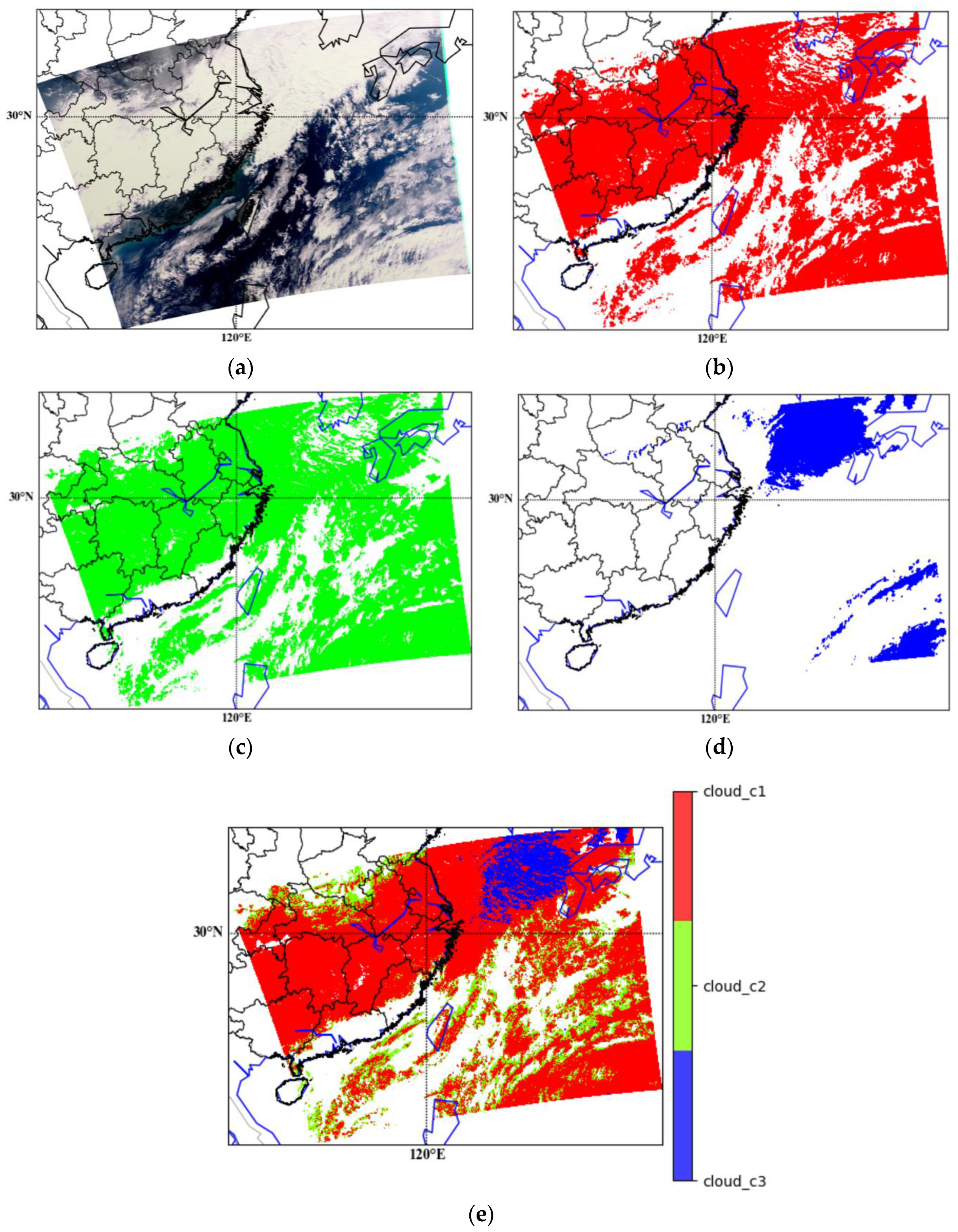
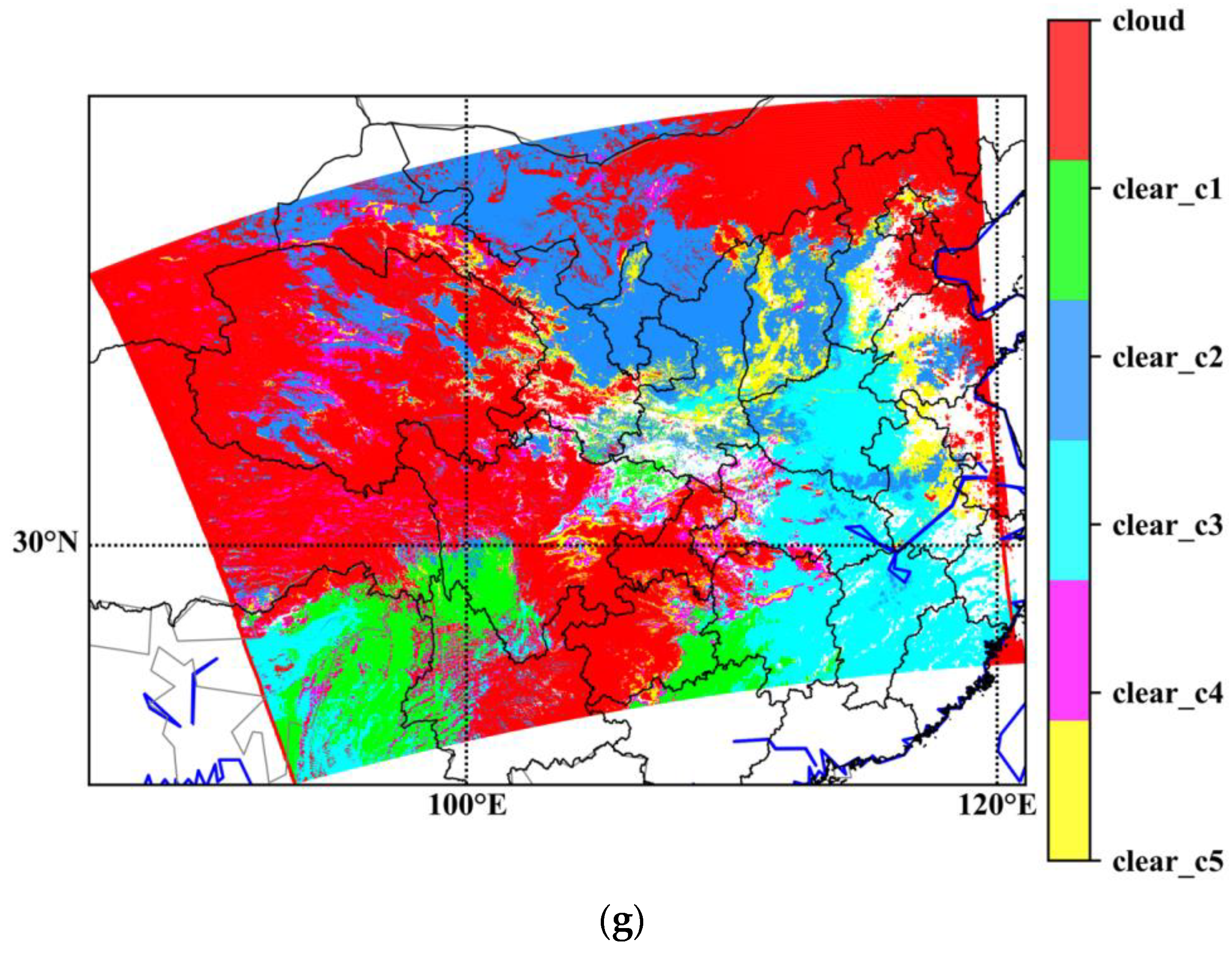
| cloud | R0.65 > 0.45 [defined as cloud_c1] | |
| R0.47_std > 0.0075 & R0.65 > 0.4 [defined as cloud_c2] | / | |
| BT11 < 250 K [defined as cloud_c3] | ||
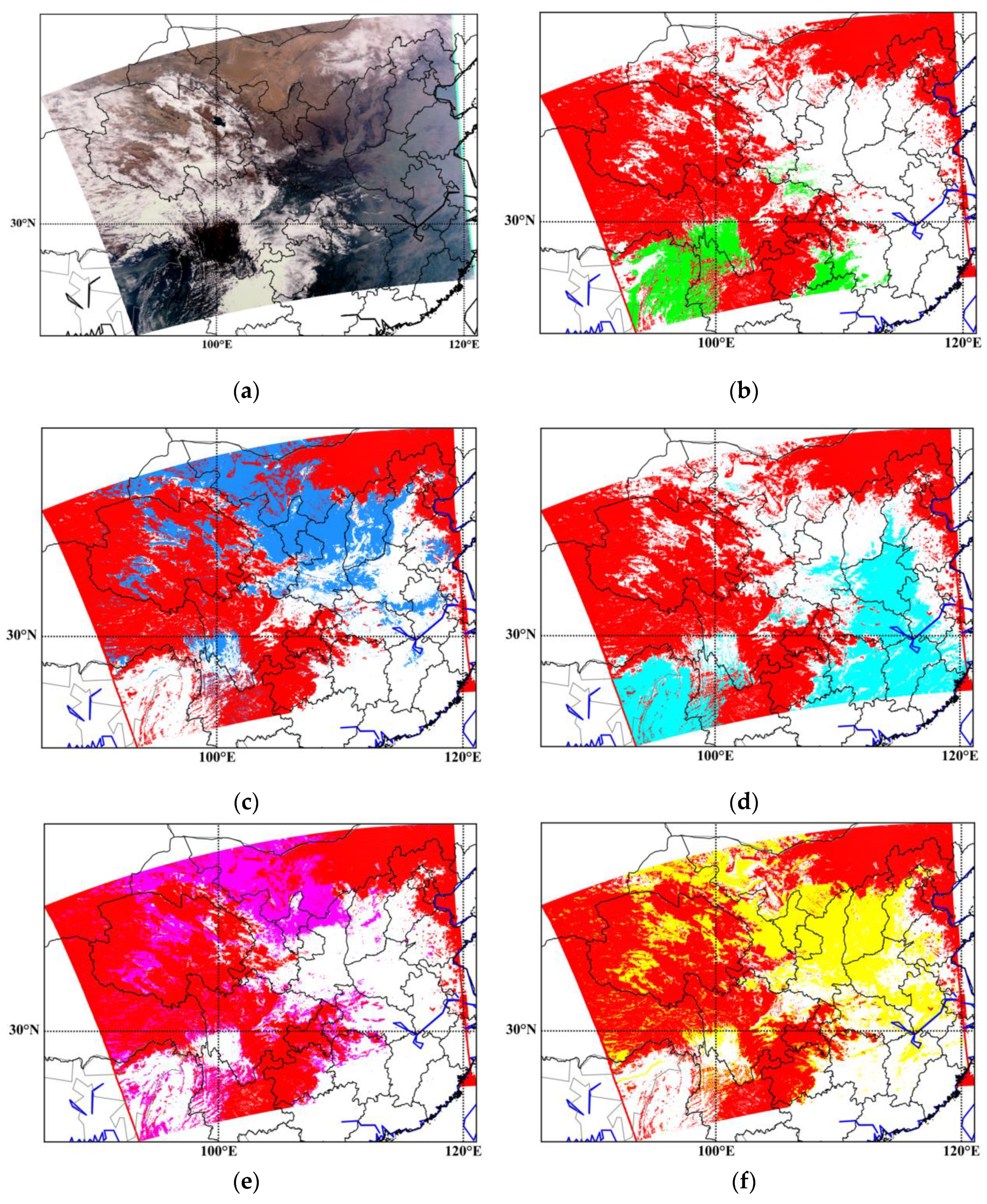
| clear | / | 0 < R0.65 < 0.2 [defined as clear_c1] |
| Diff0.865_1.64 > 0 [defined as clear_c2] | ||
| BT11 > 285 [defined as clear_c3] | ||
| BT11-BT3.8 [−50, −40] [defined as clear_c4] | ||
| 3 NDVIswir < 0.2 & 0.2 ≤ R0.65 < 0.4 [defined as clear_c5] |
| Scenarios | Selected Areas | Selected Time |
|---|---|---|
| clear1 | 42.8496~45.3657, 109.1090~113.6038 | 8 November 2019/4 April 2020/14 June 2020 |
| 42.2122~43.1121, 108.6515~109.7193 | 3 December 2019 | |
| clear2 | 23.9992~24.3478, 112.7604~113.6705 | 8 November 2019/3 December 2019 |
| 23.0716~23.7766, 115.0593~115.8996 | 2 December 2019 | |
| 25.3634~25.9159, 116.7444~117.5885 | 15 March 2020 | |
| cloud1 | 27.8471~29.0374, 103.8887~105.2329 | 8 November 2019/23 December 2019/3 April 2020/17 June 2020 |
| cloud2 | 36.1867~36.7887, 108.4950~109.3658 | 8 November 2019/24 December 2019/1 April 2020/22 June 2020 |
| haze1 | 38.0390~39.24, 115.2247~116.4105 | 8 November 2019/13 December 2019/6 April 2020/11 June 2019 |
| haze2 | 33.9950~35.4849, 113.6284~114.8294 | 8 November 2019/13 December 2019/26 April 2020/18 June 2020 |
| 34.8348~35.8514, 114.2112~115.4611 | 18 June 2019 |
| Date/Orbit | PM2.5 >= 50 μg/m3 | PM2.5 >= 35 μg/m3 | ||||
|---|---|---|---|---|---|---|
| Haze | Clear | Hit Rate (%) | Haze | Clear | Hit Rate (%) | |
| 14 January 2020-0430 | 48 | 2 | 96.00 | 76 | 5 | 93.83 |
| 19 January 2020-0435 | 163 | 2 | 98.79 | 195 | 6 | 97.01 |
| 20 January 2020-0555 | 145 | 42 | 75.94 | 190 | 66 | 74.21 |
| 28 January 2020-0505 | 201 | 33 | 85.90 | 250 | 39 | 86.51 |
| 29 January 2020-0445 | 172 | 11 | 93.99 | 220 | 18 | 92.44 |
| 30 January 2020-0425 | 74 | 2 | 97.37 | 86 | 4 | 95.56 |
| 31 January 2020-0545 | 162 | 15 | 91.53 | 242 | 28 | 89.63 |
| 31 January 2020-0550 | 129 | 61 | 67.89 | 139 | 91 | 60.43 |
| 3 February 2020-0450 | 125 | 5 | 96.15 | 198 | 18 | 91.67 |
| 9 February 2020-0435 | 95 | 0 | 100 | 144 | 2 | 98.63 |
| 4 March 2020-0520 | 53 | 0 | 100 | 94 | 1 | 98.95 |
| 4 March 2020-0525 | 14 | 2 | 87.5 | 12 | 33 | 26.67 |
| 7 March 2020-0425 | 83 | 1 | 98.81 | 98 | 2 | 98.0 |
| 7 March 2020-0430 | 10 | 0 | 100 | 12 | 12 | 100 |
| 19 October 2020-0445 | 136 | 5 | 96.45 | 193 | 12 | 94.15 |
| 21 October 2020-0545 | 64 | 11 | 85.33 | 5 | 46 | 9.80 |
| 21 October 2020-0550 | 1 | 26 | 3.70 | 127 | 34 | 78.88 |
| 22 October 2020-0525 | 91 | 5 | 94.79 | 164 | 15 | 91.62 |
Disclaimer/Publisher’s Note: The statements, opinions and data contained in all publications are solely those of the individual author(s) and contributor(s) and not of MDPI and/or the editor(s). MDPI and/or the editor(s) disclaim responsibility for any injury to people or property resulting from any ideas, methods, instructions or products referred to in the content. |
© 2023 by the authors. Licensee MDPI, Basel, Switzerland. This article is an open access article distributed under the terms and conditions of the Creative Commons Attribution (CC BY) license (https://creativecommons.org/licenses/by/4.0/).
Share and Cite
Si, Y.; Chen, L.; Zheng, Z.; Yang, L.; Wang, F.; Xu, N.; Zhang, X. A Novel Algorithm of Haze Identification Based on FY3D/MERSI-II Remote Sensing Data. Remote Sens. 2023, 15, 438. https://doi.org/10.3390/rs15020438
Si Y, Chen L, Zheng Z, Yang L, Wang F, Xu N, Zhang X. A Novel Algorithm of Haze Identification Based on FY3D/MERSI-II Remote Sensing Data. Remote Sensing. 2023; 15(2):438. https://doi.org/10.3390/rs15020438
Chicago/Turabian StyleSi, Yidan, Lin Chen, Zhaojun Zheng, Leiku Yang, Fu Wang, Na Xu, and Xingying Zhang. 2023. "A Novel Algorithm of Haze Identification Based on FY3D/MERSI-II Remote Sensing Data" Remote Sensing 15, no. 2: 438. https://doi.org/10.3390/rs15020438