
SAR2HEIGHT: Height Estimation from a Single SAR Image in Mountain Areas via Sparse Height and Proxyless Depth-Aware Penalty Neural Architecture Search for Unet

Abstract
:1. Introduction
- A height estimation network based on Unet was proposed. Sparse height information and distance map are used as additional input for higher reconstruction accuracy. The root means square error of height estimation in a mountain area can be improved from ∼315 m to about 32 m (the sparse ratio of is 0.011%).
- A customized method for generating with different sparse ratios is proposed. To accommodate for various sparse inputs, a mask function is proposed to simulate the sparse patterns.
- A proxyless depth-aware penalty neural architecture search is proposed to learn the optimal architecture for Unet.
2. Materials and Methods
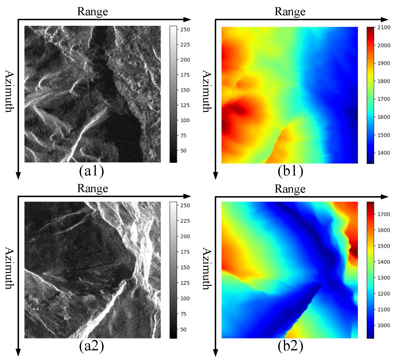
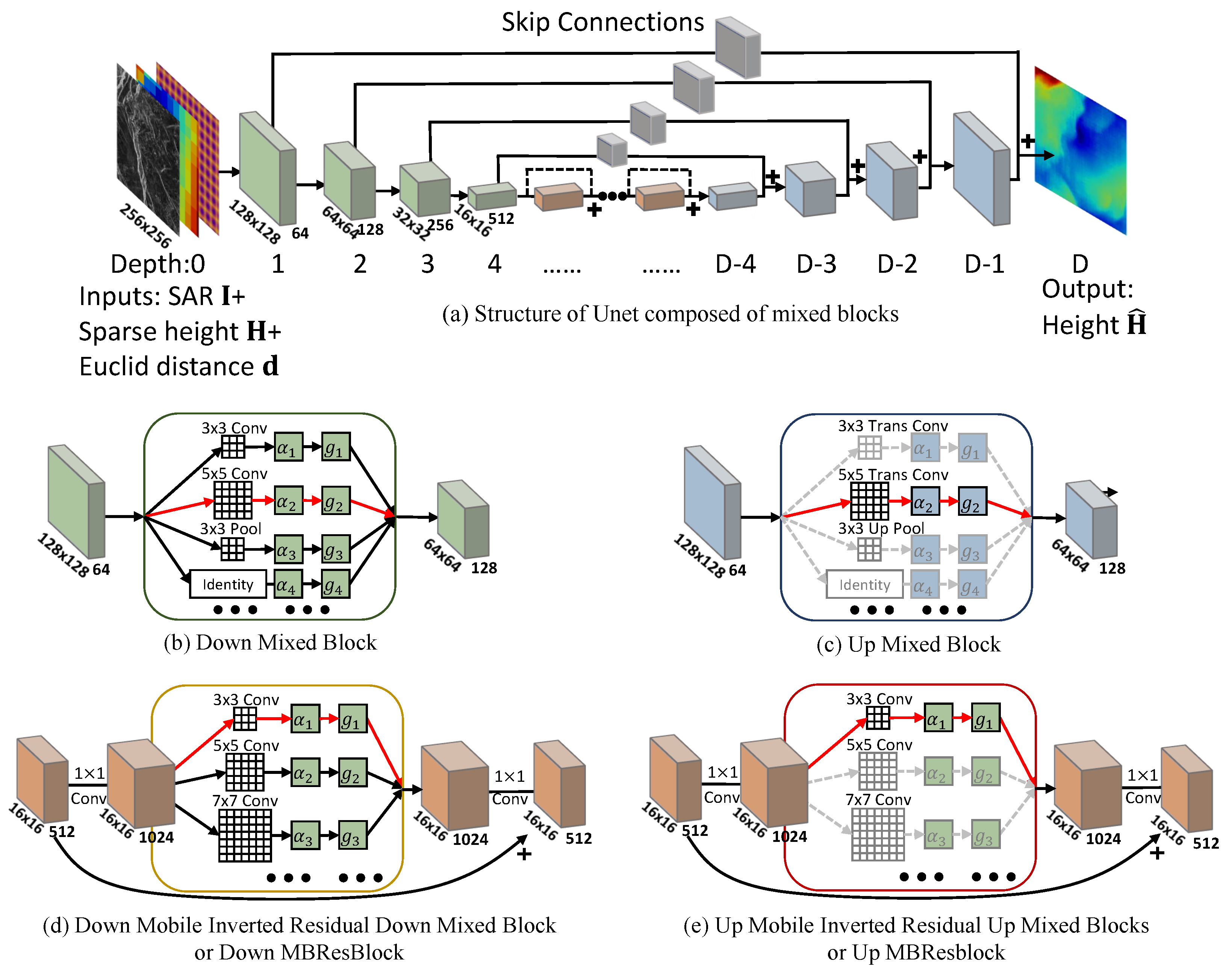
2.1. The Proposed Method
2.2. Coordinate Transformation and Image Registration
- 1.
- Establishing initial geometric transformation between SAR image and DEM based on range-Doppler (RD) model [36].
- 2.
- Refining the geometric transformation by offset calculation between SAR data and simulated SAR based on DEM.
- 3.
- Resampling image data sets from DEM to SAR coordinates system.
2.3. Parameterization of Sparse Height
| Algorithm 1 Parameterized methods for generating inputs of SAR2HEIGHT. |
|
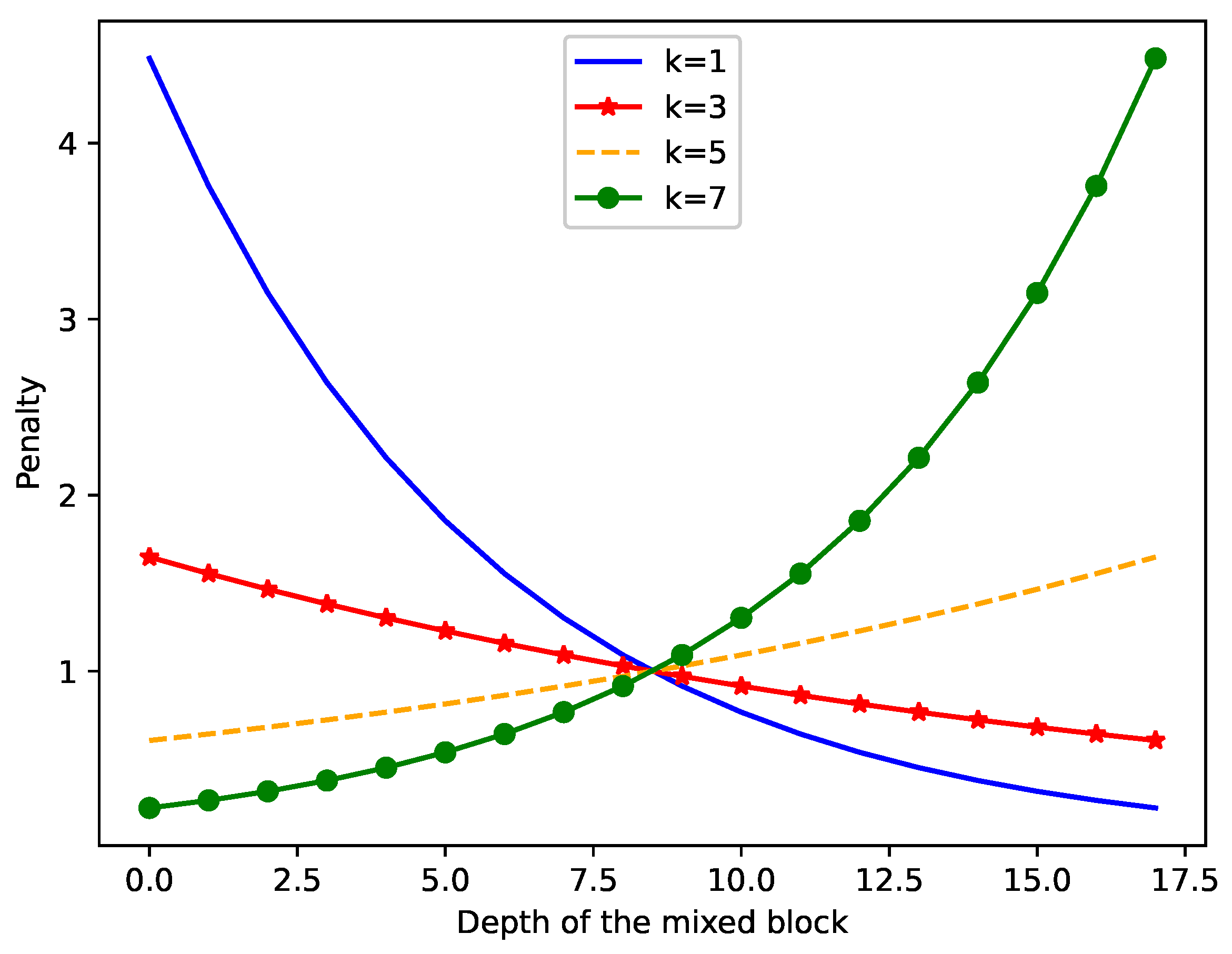
2.4. Proxyless Depth-Aware Penalty Neural Architecture Search (PDPNAS) for Unet
3. Results and Discussion
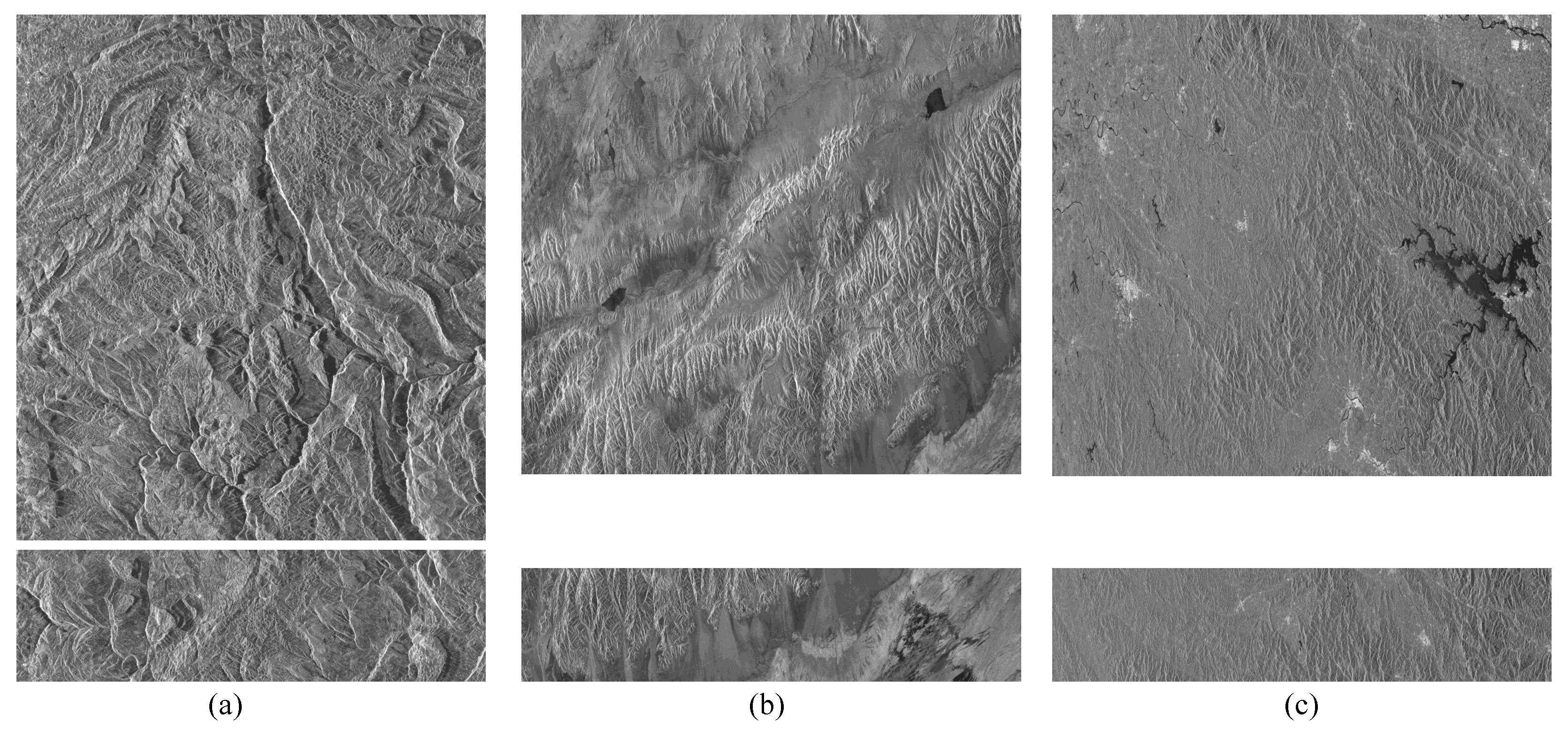
3.1. Experiment Setup
3.2. Evaluation Metrics
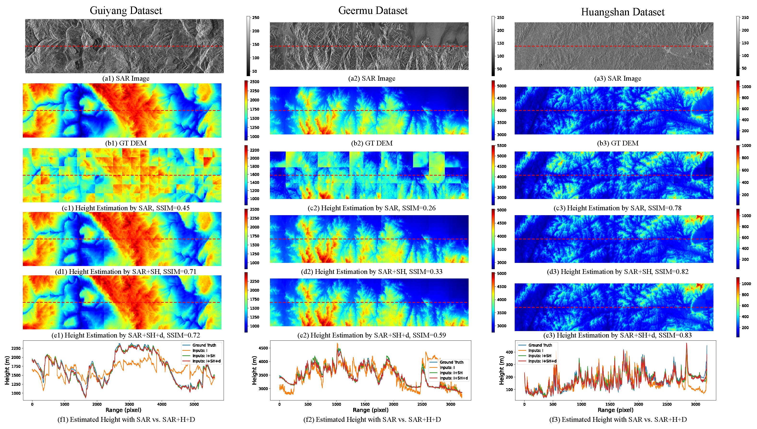
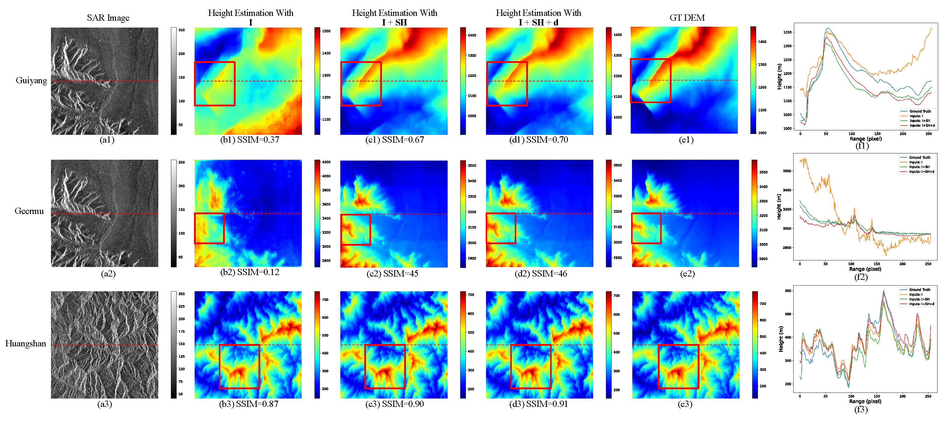
3.3. The Effect of Sparse Height Information and Distance Map
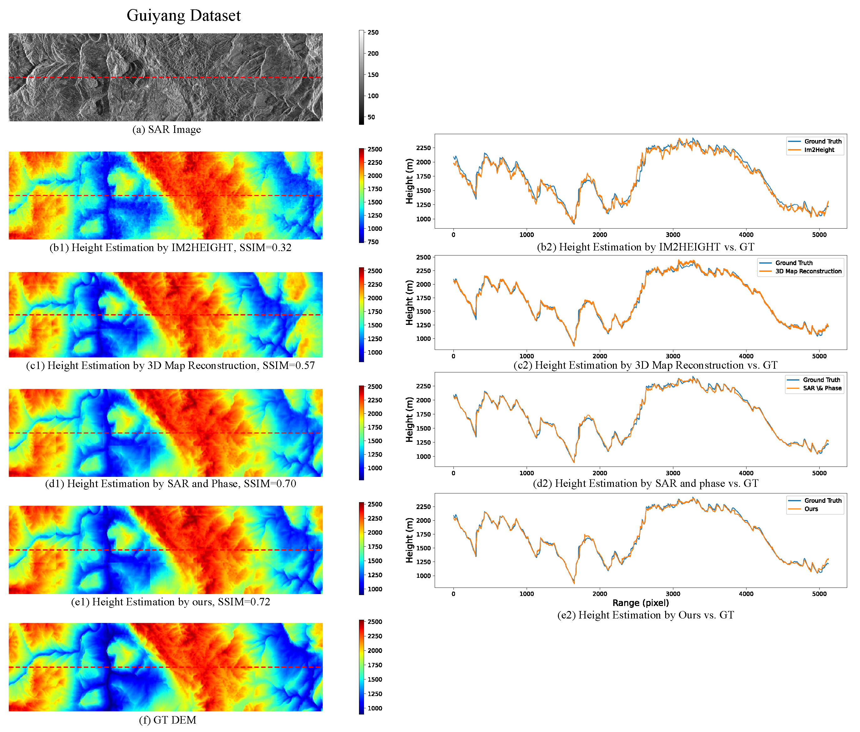
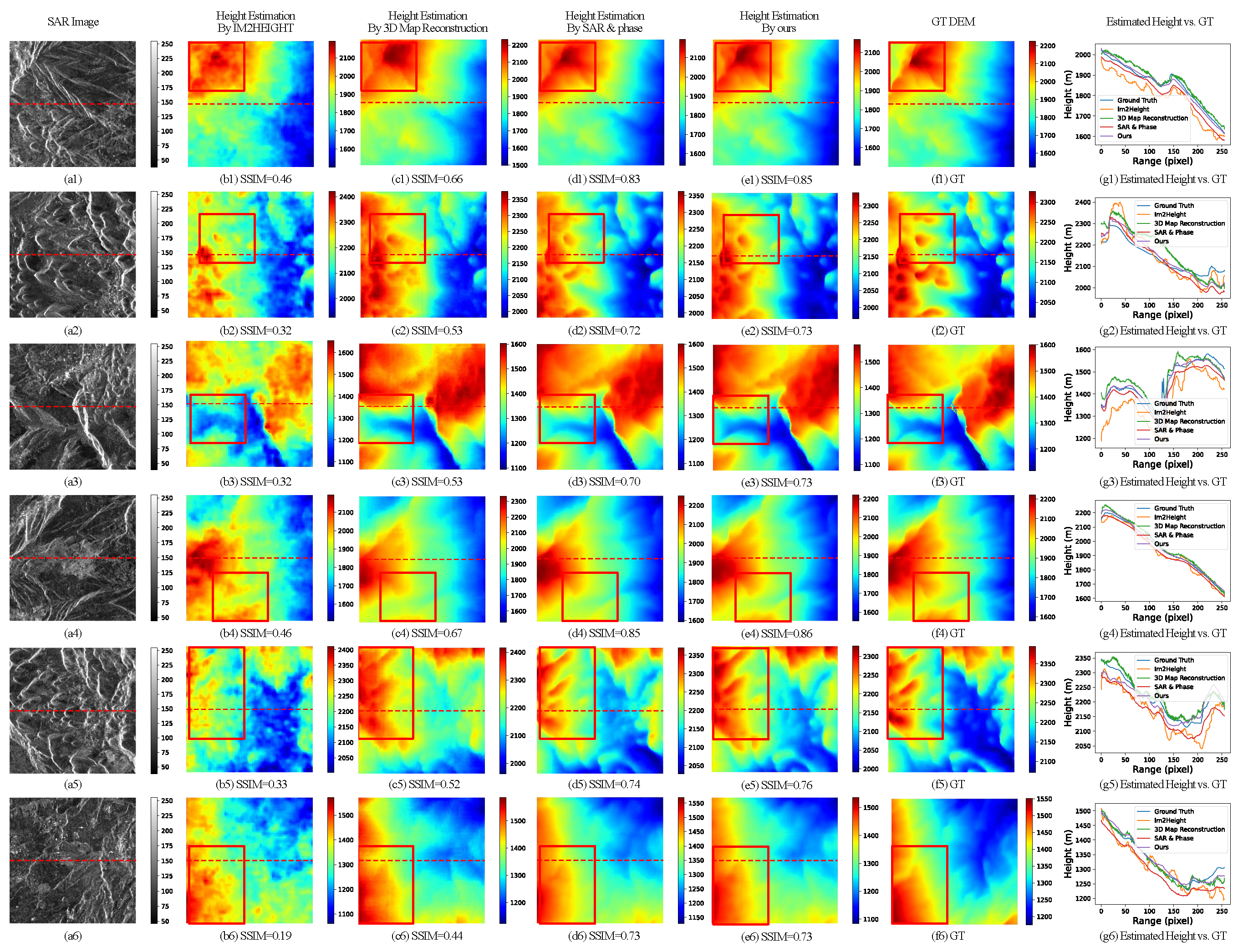
3.4. Comparison of Different Network Structures
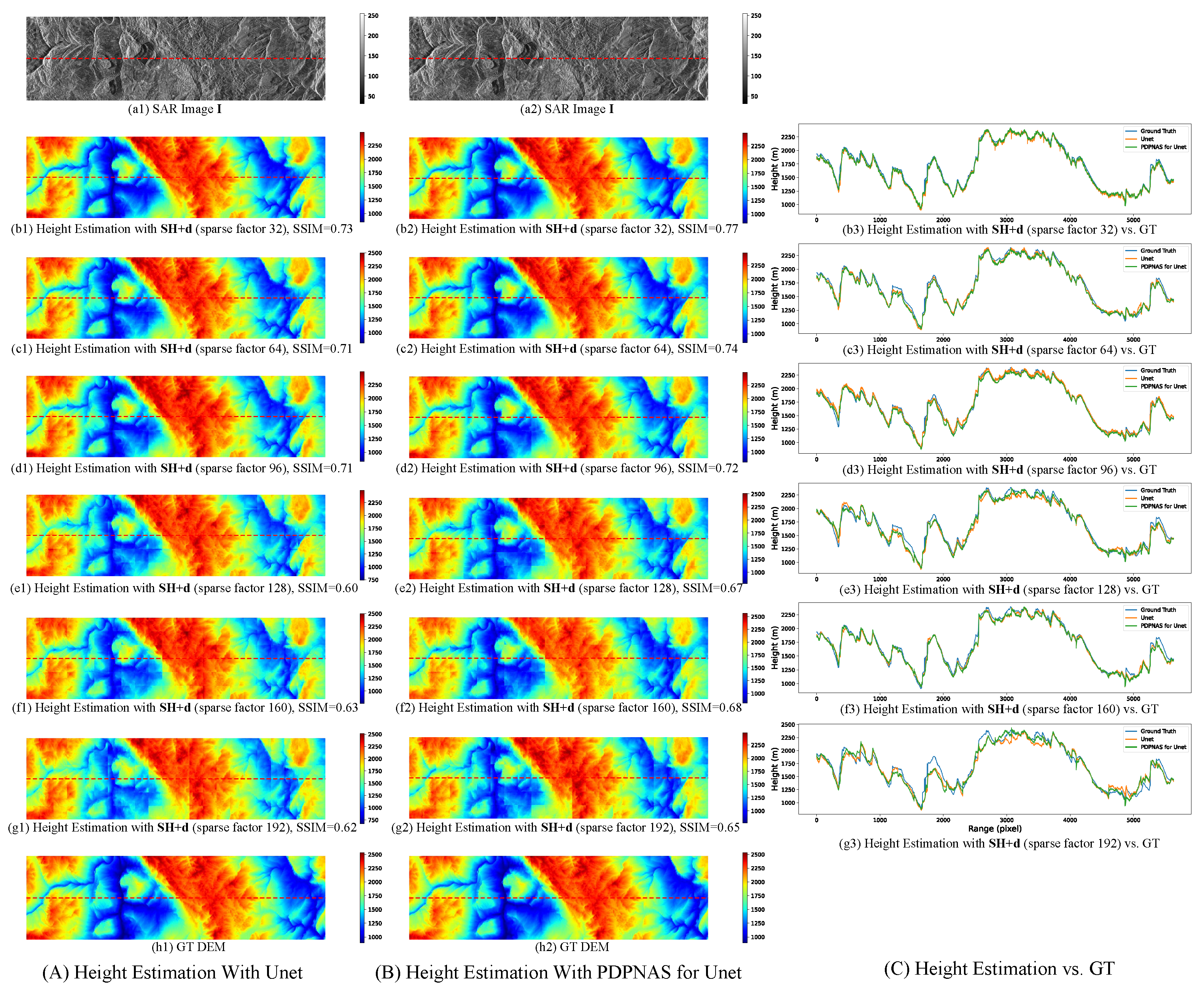
3.5. The Effect of PDPNAS
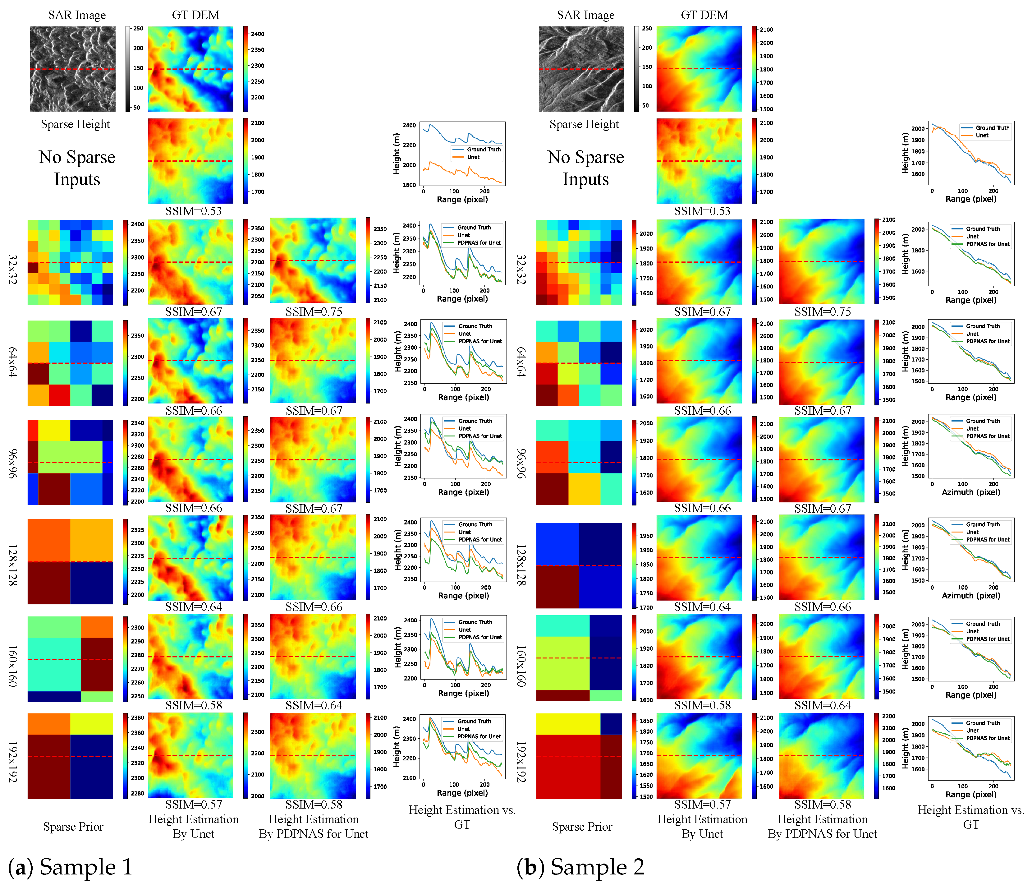
3.6. Comparison on the Effect of Sparse Height with Various Sparsity
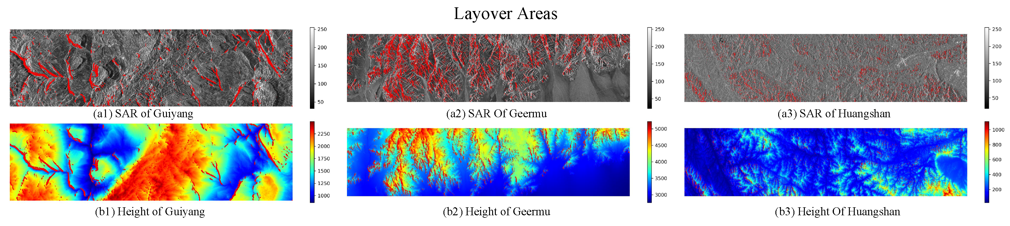
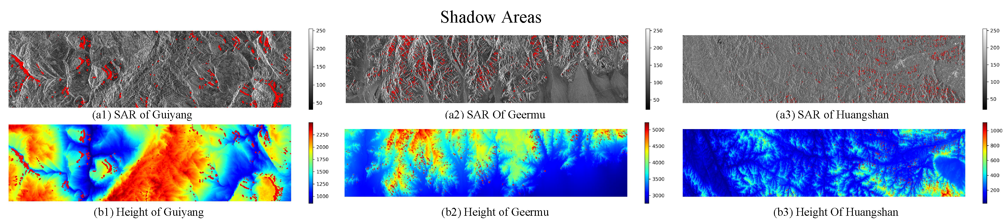
3.7. Layover and Shadow
4. Conclusions
Author Contributions
Funding
Data Availability Statement
Acknowledgments
Conflicts of Interest
References
- Rizzoli, P.; Martone, M.; Gonzalez, C.; Wecklich, C.; Tridon, D.B.; Bräutigam, B.; Bachmann, M.; Schulze, D.; Fritz, T.; Huber, M.; et al. Generation and performance assessment of the global TanDEM-X digital elevation model. ISPRS J. Photogramm. Remote Sens. 2017, 132, 119–139. [Google Scholar] [CrossRef] [Green Version]
- Hoiem, D.; Efros, A.A.; Hebert, M. Recovering surface layout from an image. Int. J. Comput. Vis. 2007, 75, 151–172. [Google Scholar] [CrossRef]
- Saxena, A.; Sun, M.; Ng, A.Y. Make3d: Learning 3d scene structure from a single still image. IEEE Trans. Pattern Anal. Mach. Intell. 2008, 31, 824–840. [Google Scholar] [CrossRef] [PubMed] [Green Version]
- Karsch, K.; Liu, C.; Kang, S.B. Depth transfer: Depth extraction from video using non-parametric sampling. IEEE Trans. Pattern Anal. Mach. Intell. 2014, 36, 2144–2158. [Google Scholar] [CrossRef] [PubMed] [Green Version]
- Mou, L.; Zhu, X.X. IM2HEIGHT: Height estimation from single monocular imagery via fully residual convolutional-deconvolutional network. arXiv 2018, arXiv:1802.10249. [Google Scholar]
- Costante, G.; Ciarfuglia, T.A.; Biondi, F. Towards monocular digital elevation model (DEM) estimation by convolutional neural networks-Application on synthetic aperture radar images. In Proceedings of the EUSAR 2018, 12th European Conference on Synthetic Aperture Radar, Aachen, Germany, 4–7 June 2018; VDE: Berlin, Germany, 2018; pp. 1–6. [Google Scholar]
- El-Darymli, K.; McGuire, P.; Power, D.; Moloney, C. Rethinking the phase in single-channel SAR imagery. In Proceedings of the 2013 14th International Radar Symposium (IRS), Dresden, Germany, 19-21 June 2013; IEEE: Piscataway, NJ, USA, 2013; Volume 1, pp. 429–436. [Google Scholar]
- Amirkolaee, H.A.; Arefi, H. Height estimation from single aerial images using a deep convolutional encoder-decoder network. ISPRS J. Photogramm. Remote Sens. 2019, 149, 50–66. [Google Scholar] [CrossRef]
- Ghamisi, P.; Yokoya, N. Img2dsm: Height simulation from single imagery using conditional generative adversarial net. IEEE Geosci. Remote Sens. Lett. 2018, 15, 794–798. [Google Scholar] [CrossRef]
- Son, C.; Park, S.Y. 3D Map Reconstruction From Single Satellite Image Using a Deep Monocular Depth Network. In Proceedings of the 2022 Thirteenth International Conference on Ubiquitous and Future Networks (ICUFN), Barcelona, Spain, 5–8 July 2022; IEEE: Piscataway, NJ, USA, 2022; pp. 5–7. [Google Scholar]
- Carvalho, M.; Le Saux, B.; Trouvé-Peloux, P.; Champagnat, F.; Almansa, A. Multitask learning of height and semantics from aerial images. IEEE Geosci. Remote Sens. Lett. 2019, 17, 1391–1395. [Google Scholar] [CrossRef] [Green Version]
- Srivastava, S.; Volpi, M.; Tuia, D. Joint height estimation and semantic labeling of monocular aerial images with CNNs. In Proceedings of the 2017 IEEE International Geoscience and Remote Sensing Symposium (IGARSS), Fort Worth, TX, USA, 23–28 July 2017; IEEE: Piscataway, NJ, USA, 2017; pp. 5173–5176. [Google Scholar]
- Zamir, A.R.; Sax, A.; Shen, W.; Guibas, L.J.; Malik, J.; Savarese, S. Taskonomy: Disentangling task transfer learning. In Proceedings of the IEEE Conference on Computer Vision and Pattern Recognition, Salt Lake City, UT, USA, 18–22 June 2018; pp. 3712–3722. [Google Scholar]
- Mahmud, J.; Price, T.; Bapat, A.; Frahm, J.M. Boundary-aware 3D building reconstruction from a single overhead image. In Proceedings of the IEEE/CVF Conference on Computer Vision and Pattern Recognition, Seattle, WA, USA, 14–19 June 2020; pp. 441–451. [Google Scholar]
- Mallya, A.; Lazebnik, S. Packnet: Adding multiple tasks to a single network by iterative pruning. In Proceedings of the IEEE Conference on Computer Vision and Pattern Recognition, Salt Lake City, UT, USA, 18–22 June 2018; pp. 7765–7773. [Google Scholar]
- Liu, C.J.; Krylov, V.A.; Kane, P.; Kavanagh, G.; Dahyot, R. IM2ELEVATION: Building height estimation from single-view aerial imagery. Remote Sens. 2020, 12, 2719. [Google Scholar] [CrossRef]
- Amini Amirkolaee, H.; Arefi, H. Generating a highly detailed DSM from a single high-resolution satellite image and an SRTM elevation model. Remote Sens. Lett. 2021, 12, 335–344. [Google Scholar] [CrossRef]
- Kim, J.; Lee, J.K.; Lee, K.M. Accurate image super-resolution using very deep convolutional networks. In Proceedings of the IEEE Conference on Computer Vision and Pattern Recognition, Las Vegas, NV, USA, 27–30 June 2016; pp. 1646–1654. [Google Scholar]
- Xia, Z.; Sullivan, P.; Chakrabarti, A. Generating and exploiting probabilistic monocular depth estimates. In Proceedings of the IEEE/CVF Conference on Computer Vision and Pattern Recognition, Seattle, WA, USA, 14–19 June 2020; pp. 65–74. [Google Scholar]
- Pravitasari, A.A.; Iriawan, N.; Almuhayar, M.; Azmi, T.; Irhamah, I.; Fithriasari, K.; Purnami, S.W.; Ferriastuti, W. UNet-VGG16 with transfer learning for MRI-based brain tumor segmentation. TELKOMNIKA (Telecommun. Comput. Electron. Control) 2020, 18, 1310–1318. [Google Scholar] [CrossRef]
- Pellegrin, L.; Martinez-Carranza, J. Towards depth estimation in a single aerial image. Int. J. Remote Sens. 2020, 41, 1970–1985. [Google Scholar] [CrossRef]
- Stan, S.; Rostami, M. Unsupervised model adaptation for continual semantic segmentation. In Proceedings of the AAAI Conference on Artificial Intelligence, Virtual, 2–9 February 2021; Volume 35, pp. 2593–2601. [Google Scholar]
- Wibowo, A.; Triadyaksa, P.; Sugiharto, A.; Sarwoko, E.A.; Nugroho, F.A.; Arai, H.; Kawakubo, M. Cardiac Disease Classification Using Two-Dimensional Thickness and Few-Shot Learning Based on Magnetic Resonance Imaging Image Segmentation. J. Imaging 2022, 8, 194. [Google Scholar] [CrossRef]
- Simon, C.; Koniusz, P.; Nock, R.; Harandi, M. Adaptive subspaces for few-shot learning. In Proceedings of the IEEE/CVF Conference on Computer Vision and Pattern Recognition, Seattle, WA, USA, 14–19 June 2020; pp. 4136–4145. [Google Scholar]
- Zhang, J.; Xing, M.; Sun, G.C.; Shi, X. Vehicle Trace Detection in Two-Pass SAR Coherent Change Detection Images With Spatial Feature Enhanced Unet and Adaptive Augmentation. IEEE Trans. Geosci. Remote Sens. 2022, 60, 1–15. [Google Scholar] [CrossRef]
- Bender, G.; Kindermans, P.J.; Zoph, B.; Vasudevan, V.; Le, Q. Understanding and simplifying one-shot architecture search. In Proceedings of the International Conference on Machine Learning, Stockholm, Sweden, 10–15 July 2018; PMLR: London, UK, 2018; pp. 550–559. [Google Scholar]
- Liu, H.; Simonyan, K.; Yang, Y. Darts: Differentiable architecture search. arXiv 2018, arXiv:1806.09055. [Google Scholar]
- Cai, H.; Zhu, L.; Han, S. ProxylessNAS: Direct Neural Architecture Search on Target Task and Hardware. In Proceedings of the International Conference on Learning Representations, New Orleans, LA, USA, 6–9 May 2019. [Google Scholar]
- Weng, Y.; Zhou, T.; Li, Y.; Qiu, X. Nas-unet: Neural architecture search for medical image segmentation. IEEE Access 2019, 7, 44247–44257. [Google Scholar] [CrossRef]
- Park, Y.; Guldmann, J.M. Creating 3D city models with building footprints and LIDAR point cloud classification: A machine learning approach. Comput. Environ. Urban Syst. 2019, 75, 76–89. [Google Scholar] [CrossRef]
- Bao, Y.; Tang, L.; Srinivasan, S.; Schnable, P.S. Field-based architectural traits characterisation of maize plant using time-of-flight 3D imaging. Biosyst. Eng. 2019, 178, 86–101. [Google Scholar] [CrossRef]
- Honkavaara, E.; Saari, H.; Kaivosoja, J.; Pölönen, I.; Hakala, T.; Litkey, P.; Mäkynen, J.; Pesonen, L. Processing and assessment of spectrometric, stereoscopic imagery collected using a lightweight UAV spectral camera for precision agriculture. Remote Sens. 2013, 5, 5006–5039. [Google Scholar] [CrossRef] [Green Version]
- Gonçalves, J.; Henriques, R. UAV photogrammetry for topographic monitoring of coastal areas. ISPRS J. Photogramm. Remote Sens. 2015, 104, 101–111. [Google Scholar] [CrossRef]
- Xu, B.; Wang, N.; Chen, T.; Li, M. Empirical evaluation of rectified activations in convolutional network. arXiv 2015, arXiv:1505.00853. [Google Scholar]
- Luo, Q.; Zhang, J.; Hui, L. A Geocoding Method for Interferometric DEM in Difficult Mapping Areas. In Proceedings of the 31st of Asian Conference on Remote Sensing, Hanoi, Vietnam, 1–5 November 2010; pp. 1298–1304. [Google Scholar]
- Luo, Y.; Qiu, X.; Dong, Q.; Fu, K. A Robust Stereo Positioning Solution for Multiview Spaceborne SAR Images Based on the Range–Doppler Model. IEEE Geosci. Remote Sens. Lett. 2021, 19, 1–5. [Google Scholar] [CrossRef]
- Luo, Q.; Hu, M.; Zhao, Z.; Li, J.; Zeng, Z. Design and experiments of X-type artificial control targets for a UAV-LiDAR system. Int. J. Remote Sens. 2020, 41, 3307–3321. [Google Scholar] [CrossRef]
- Xi, Y.; Luo, Q. A morphology-based method for building change detection using multi-temporal airborne LiDAR data. Remote Sens. Lett. 2018, 9, 131–139. [Google Scholar] [CrossRef]
- Sandler, M.; Howard, A.; Zhu, M.; Zhmoginov, A.; Chen, L.C. Mobilenetv2: Inverted residuals and linear bottlenecks. In Proceedings of the IEEE Conference on Computer Vision and Pattern Recognition, Salt Lake City, UT, USA, 18–22 June 2018; pp. 4510–4520. [Google Scholar]


| Layer | Kernel Size | Operation | Strides | Depth | Output Size | |
|---|---|---|---|---|---|---|
| Input | 0 | |||||
| Down1 | Conv/Down Pool | 2 | 1 | |||
| Down | Down2 | Conv/Pool | 2 | 2 | ||
| Subnetwork | Down3 | Conv/Pool | 2 | 3 | ||
| 5× | [Conv1 | Conv | 1 | |||
| Down | Conv2 | Conv | 1 | 3 + i | ||
| [MBResblocks] | Conv3] | Conv | 1 | |||
| 5× | [Conv1 | Conv | 1 | |||
| Up | Conv2 | Conv | 1 | D-3 − i | ||
| [MBResblocks] | Conv3] | Conv | 1 | |||
| Up1 | match with Down3 | 2 | D-3 | |||
| Up | Up2 | match with Down2 | 2 | D-2 | ||
| Subnetwork | Up3 | match with Down1 | 2 | D-1 | ||
| Output | Out | Conv | 2 | D |
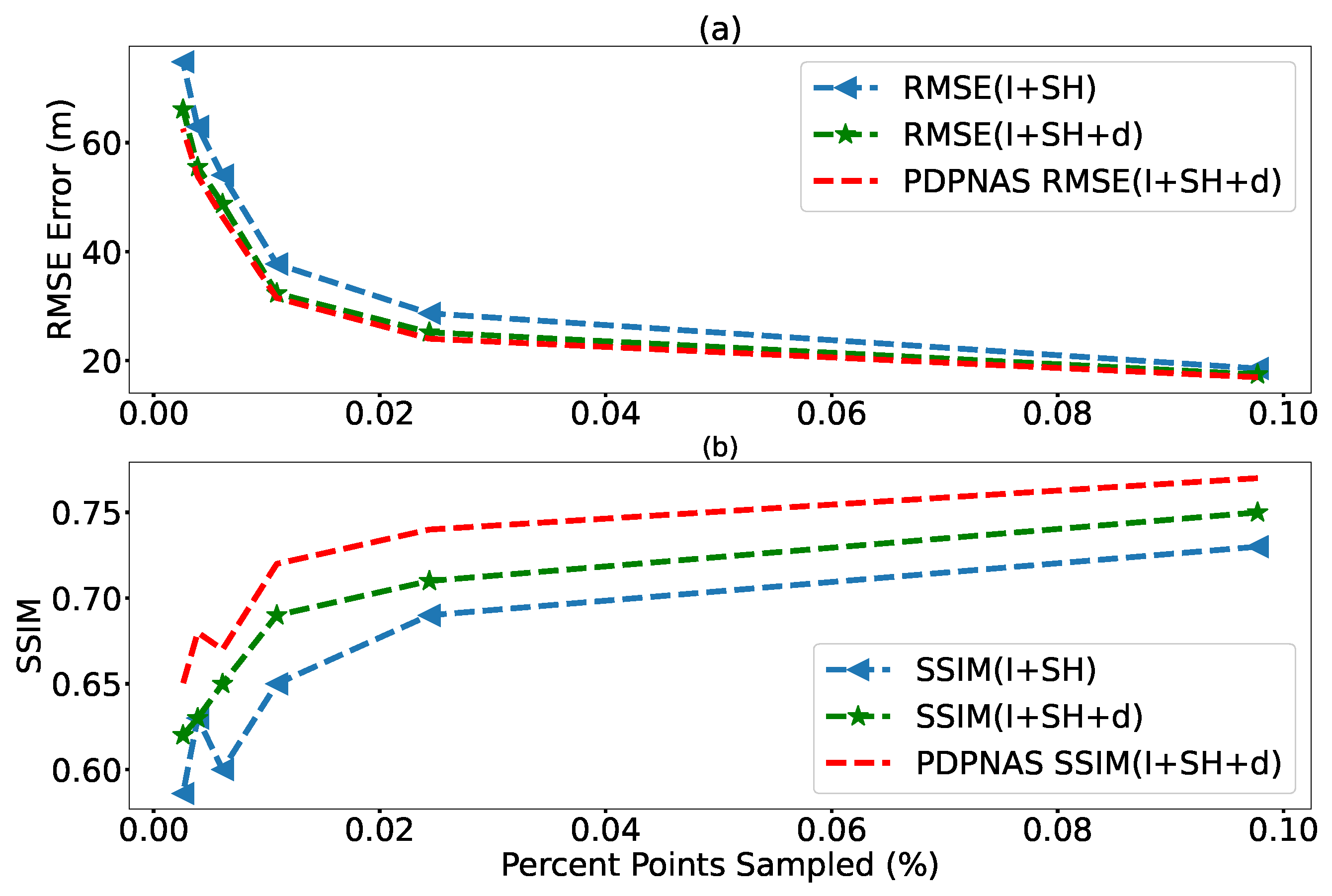
| Datasets | Downsample Factors | % Points Sampled | Inputs | Include PDPNAS | RMSE (m) | SSIM |
|---|---|---|---|---|---|---|
| Guiyang | — | — | I | No | 326.74 ± 10.75 | 0.40 ± 0.05 |
| 32 × 32 | 0.0976 | SH | No | 30.28 ± 0.25 | 0.52 ± 1 × 10⁻³ | |
| I+SH | No | 17.94 ± 0.63 | 0.72 ± 3 × 10⁻³ | |||
| I+SH+d | No | 17.49 ± 0.79 | 0.75 ± 1 × 10⁻³ | |||
| I+SH+d | Yes | 15.70 ± 0.70 | 0.78 ± 7 × 10⁻³ | |||
| 64 × 64 | 0.0244 | SH | No | 59.02 ± 0.69 | 0.28 + 2 × 10⁻³ | |
| I+SH | No | 29.45 ± 1.61 | 0.68 ± 3 × 10⁻³ | |||
| I+SH+d | No | 26.65 ± 1.63 | 0.70 ± 0.03 | |||
| I+SH+d | Yes | 24.18 ± 0.28 | 0.74 ± 2 × 10⁻³ | |||
| 96 × 96 | 0.0109 | SH | No | 78.40 ± 1.54 | 0.24 ± 4 × 10⁻³ | |
| I+SH | No | 37.84 ± 0.43 | 0.68 ± 6 × 10⁻³ | |||
| I+SH+d | No | 32.95 ± 0.65 | 0.70 ± 6 × 10⁻³ | |||
| I+SH+d | Yes | 31.70 ± 0.14 | 0.72 ± 5 × 10⁻³ | |||
| 128 × 128 | 0.0061 | SH | No | 109.91 ± 0.77 | 0.15 ± 2 × 10⁻³ | |
| I+SH | No | 53.60 ± 0.46 | 0.64 ± 7 × 10⁻³ | |||
| I+SH+d | No | 46.56 ± 0.46 | 0.64 ± 0.02 | |||
| I+SH+d | Yes | 45.01 ± 0.57 | 0.68 ± 7 × 10⁻³ | |||
| 160 × 160 | 0.0039 | SH | No | 117.72 ± 0.79 | 0.14 ± 1 × 10⁻³ | |
| I+SH | No | 63.65 ± 0.52 | 0.63 ± 5 × 10⁻³ | |||
| I+SH+d | No | 56.27 ± 0.56 | 0.63 ± 1 × 10⁻³ | |||
| I+SH+d | Yes | 53.94 ± 0.44 | 0.68 ± 1 × 10⁻³ | |||
| 192 × 192 | 0.0027 | SH | No | 145.83 ± 1.41 | 0.11 ± 3 × 10⁻³ | |
| I+SH | No | 74.03 ± 1.296 | 0.59 + 7 × 10⁻³ | |||
| I+SH+d | No | 65.39 ± 0.54 | 0.62 ± 4 × 10⁻³ | |||
| I+SH+d | Yes | 62.55 ± 0.42 | 0.64 ± 0.08 | |||
| Geermu | — | — | I | Yes | 1015.22 ± 43.63 | 0.27 ± 0.01 |
| 64 × 64 | 0.0244 | SH | Yes | 90.96 ± 1.27 | 0.07 ± 3 × 10⁻³ | |
| I+SH | Yes | 41.61 ± 1.53 | 0.36 ± 9 × 10⁻³ | |||
| I+SH+d | Yes | 29.77 ± 1.48 | 0.36 ± 6 × 10⁻³ | |||
| 96 × 96 | 0.0109 | SH | Yes | 77.42 ± 1.74 | 0.25 ± 4 × 10⁻³ | |
| I+SH | Yes | 43.18 ± 1.25 | 0.36 ± 9 × 10⁻³ | |||
| I+SH+d | Yes | 41.61 ± 1.53 | 0.37 ± 5 × 10⁻³ | |||
| 128 × 128 | 0.0061 | SH | Yes | 145.82 ± 2.13 | 0.03 ± 0.11 | |
| I+SH | Yes | 65.44 ± 4.15 | 0.35 ± 6 × 10⁻³ | |||
| I+SH+d | Yes | 63.93 ± 2.831 | 0.37 ± 2 × 10⁻³ | |||
| Huangshan | — | — | I | Yes | 124.16 ± 3.18 | 0.780 ± 5 × 10⁻³ |
| 64 × 64 | 0.0244 | SH | Yes | 108.12 ± 0.40 | 0.06 ± 1 × 10⁻³ | |
| I+SH | Yes | 36.00 ± 1.05 | 0.81 ± 6 × 10⁻³ | |||
| I+SH+d | Yes | 29.98 ± 2.80 | 0.83 ± 2 × 10⁻³ | |||
| 96 × 96 | 0.0109 | SH | Yes | 123.82 ± 0.36 | 0.04 ± 1 × 10⁻³ | |
| I+SH | Yes | 49.06 ± 2.84 | 0.81 ± 4 × 10⁻³ | |||
| I+SH+d | Yes | 37.02 ± 0.63 | 0.83 ± 2 × 10⁻³ | |||
| 128 × 128 | 0.0061 | SH | Yes | 161.71 ± 0.58 | 0.02 ± 2 × 10⁻³ | |
| I+SH | Yes | 60.14 ± 1.03 | 0.81 ± 0.006 | |||
| I+SH+d | Yes | 45.77 ± 1.26 | 0.82 ± 2 × 10⁻³ |
| Method | Inputs | Structure of Unet Same to Us | Include PDPNAS | RMSE (m) | SSIM |
|---|---|---|---|---|---|
| VDSR [18] | I+SH+d | No | No | 79.36 ± 6.92 | 0.31 ± 6 × 10⁻³ |
| PackNet [15] | I+SH+d | No | No | 59.55 ± 1.80 | 0.49 ± 2 × 10⁻³ |
| IM2HEIGHT [5] | I+SH+d | No | No | 52.89 ± 0.37 | 0.31 ± 5 × 10⁻³ |
| 3DMap [10] | I+SH+d | Yes | No | 37.17 ± 1.11 | 0.54 ± 0.01 |
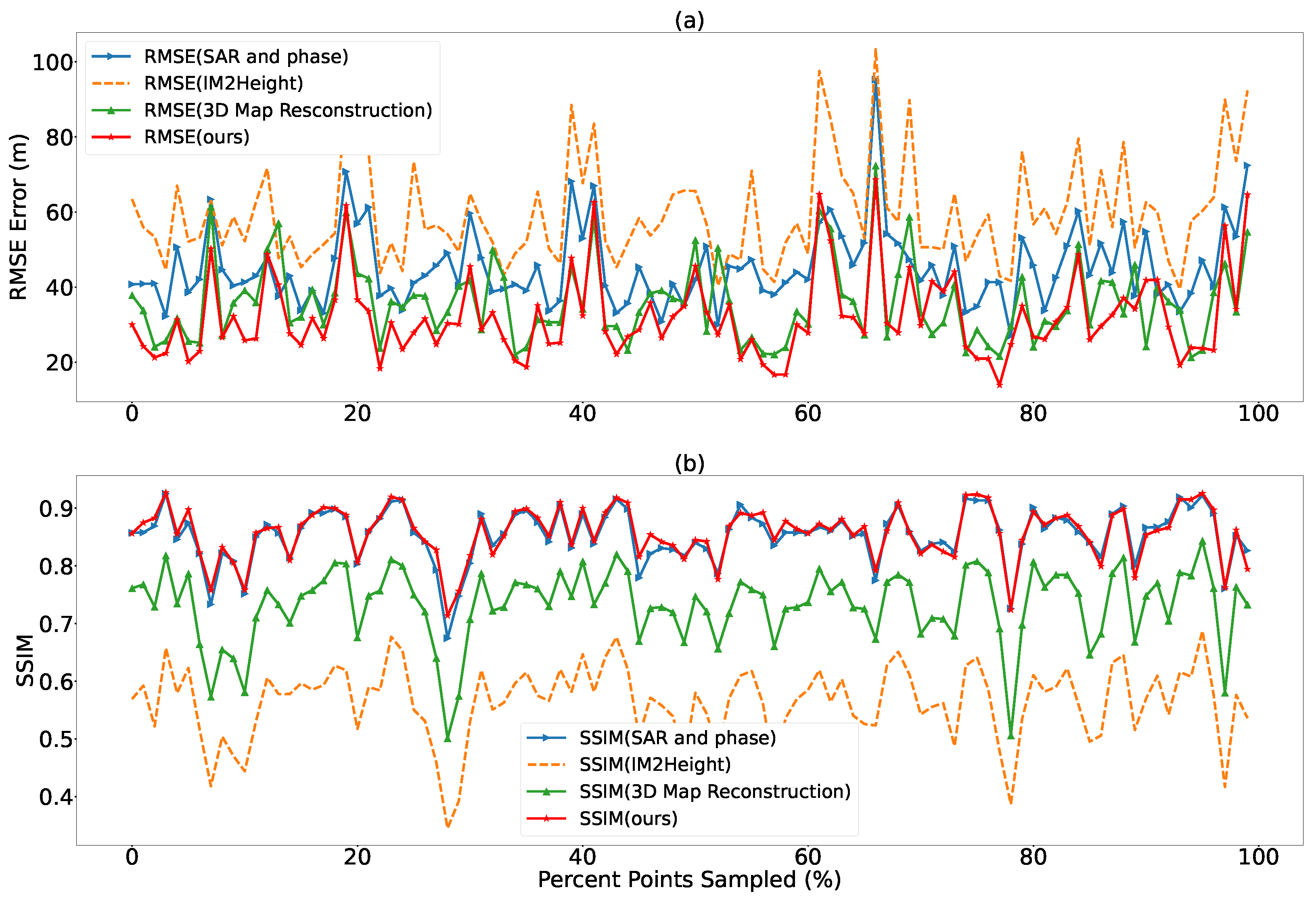
| SAR&phase [6] | I+phase | No | No | 392.22 ± 3.68 | 0.01 ± 3 × 10⁻³ |
| I+SH+d+phase | Yes | No | 33.48 ± 0.25 | 0.72 ± 5 × 10⁻³ | |
| ours | I+SH+d | Yes | No | 32.95 ± 0.65 | 0.70 ± 6 × 10⁻³ |
| Yes | Yes | 31.70 ± 0.14 | 0.73 ± 5 × 10⁻³ |
| Methods | Include MBResblocks | Is Symmteric | Includes Depth-Aware Penalty | RMSE (m) | SSIM |
|---|---|---|---|---|---|
| Unet | Yes | Yes | No | 32.95 ± 0.65 | 0.70 ± 6 × 10⁻³ |
| NAS-Unet | Yes | No | No | 33.54 ± 0.63 | 0.69 ± 0.01 |
| PDPNAS for Unet | No | Yes | Yes | 52.89 ± 0.37 | 0.31 ± 5 × 10⁻³ |
| Yes | No | Yes | 32.67 ± 0.34 | 0.71 ± 3 × 10⁻³ | |
| Yes | Yes | Yes | 31.70 ± 0.14 | 0.72 ± 5 × 10⁻³ |
| Datasets | Downsample Factors | % Points Sampled | Include Layover | Include Shadow | Include Others | RMSE (m) | MARE (%) |
|---|---|---|---|---|---|---|---|
| Guiyang | 32 × 32 | 0.0976 | Yes | Yes | Yes | 15.70 ± 0.70 | 0.54 ± 3 × 10⁻³ |
| Yes | No | No | 72.73 ± 1.41 | 3.47 ± 0.01 | |||
| No | Yes | No | 15.87 ± 0.63 | 0.66 ± 9 × 10⁻³ | |||
| No | No | Yes | 12.39 ± 0.19 | 0.50 ± 4 × 10⁻³ | |||
| 64 × 64 | 0.0244 | Yes | Yes | Yes | 23.38 ± 0.28 | 1.00 ± 2 × 10⁻³ | |
| Yes | No | No | 81.71 ± 1.32 | 4.14 ± 0.01 | |||
| No | Yes | No | 24.60 ± 0.62 | 1.17 ± 2 × 10⁻³ | |||
| No | No | Yes | 21.52 ± 0.39 | 0.95 ± 7 × 10⁻³ | |||
| 96 × 96 | 0.0109 | Yes | Yes | Yes | 31.70 ± 0.14 | 1.38 ± 2 × 10⁻³ | |
| Yes | No | No | 93.25 ± 1.46 | 4.78 ± 0.02 | |||
| No | Yes | No | 31.66 ± 0.65 | 1.45 ± 3 × 10⁻³ | |||
| No | No | Yes | 30.09 ± 0.18 | 1.33 ± 8 × 10⁻³ | |||
| 128 × 128 | 0.0061 | Yes | Yes | Yes | 45.01 ± 0.57 | 2.01 ± 4 × 10⁻³ | |
| Yes | No | No | 104.45 ± 1.60 | 5.62 ± 0.01 | |||
| No | Yes | No | 56.30 ± 0.55 | 2.54 ± 6 × 10⁻³ | |||
| No | No | Yes | 43.11 ± 0.35 | 1.96 ± 3 × 10⁻³ | |||
| 160 × 160 | 0.0039 | Yes | Yes | Yes | 53.94 ± 0.44 | 2.38 ± 1 × 10⁻³ | |
| Yes | No | No | 119.69 ± 1.45 | 6.53 ± 0.01 | |||
| No | Yes | No | 57.91 ± 0.88 | 2.67 ± 1 × 10⁻³ | |||
| No | No | Yes | 50.52 ± 0.76 | 2.32 ± 1 × 10⁻³ | |||
| 192 × 192 | 0.0027 | Yes | Yes | Yes | 62.55 ± 0.42 | 2.88 ± 2 × 10⁻³ | |
| Yes | No | No | 114.76 ± 1.87 | 6.19 ± 0.02 | |||
| No | Yes | No | 65.64 ± 1.07 | 3.18 ± 5 × 10⁻³ | |||
| No | No | Yes | 60.96 ± 0.80 | 2.84 ± 1 × 10⁻³ | |||
| Geermu | 64 × 64 | 0.0244 | Yes | Yes | Yes | 29.77 ± 1.48 | 0.46 ± 1 × 10⁻³ |
| Yes | No | No | 67.82 ± 1.58 | 1.28 ± 0.03 | |||
| No | Yes | No | 37.62 ± 1.16 | 0.72 ± 0.01 | |||
| No | No | Yes | 25.06 ± 0.23 | 0.45 ± 1 × 10⁻³ | |||
| 96 × 96 | 0.0109 | Yes | Yes | Yes | 41.61 ± 1.53 | 0.72 ± 1 × 10⁻³ | |
| Yes | No | No | 87.17 ± 1.40 | 1.69 ± 0.01 | |||
| No | Yes | No | 57.58 ± 1.10 | 1.15 ± 4 × 10⁻³ | |||
| No | No | Yes | 39.16 ± 0.61 | 0.70 ± 1 × 10⁻³ | |||
| 128 × 128 | 0.0061 | Yes | Yes | Yes | 63.93 ± 2.83 | 1.01 ± 1 × 10⁻³ | |
| Yes | No | No | 125.83 ± 1.39 | 2.54 ± 0.01 | |||
| No | Yes | No | 101.13 ± 1.51 | 2.10 ± 4 × 10⁻³ | |||
| No | No | Yes | 55.90 ± 0.26 | 0.99 ± 1 × 10⁻³ | |||
| Huangshan | 64 × 64 | 0.0244 | Yes | Yes | Yes | 29.98 ± 2.80 | 5.58 ± 0.06 |
| Yes | No | No | 43.90 ± 1.36 | 6.26 ± 0.03 | |||
| No | Yes | No | 34.74 ± 1.51 | 6.23 ± 0.01 | |||
| No | No | Yes | 23.23 ± 0.16 | 3.92 ± 0.02 | |||
| 96 × 96 | 0.0109 | Yes | Yes | Yes | 37.02 ± 0.63 | 7.85 ± 0.02 | |
| Yes | No | No | 49.25 ± 1.44 | 8.91 ± 0.02 | |||
| No | Yes | No | 47.35 ± 1.36 | 8.87 ± 0.04 | |||
| No | No | Yes | 33.77 ± 0.44 | 6.76 ± 0.01 | |||
| 128 × 128 | 0.0061 | Yes | Yes | Yes | 45.77 ± 1.26 | 9.25 ± 0.10 | |
| Yes | No | No | 59.04 ± 1.74 | 10.83 ± 0.80 | |||
| No | Yes | No | 58.82 ± 0.31 | 10.78 ± 0.30 | |||
| No | No | Yes | 42.69 ± 0.66 | 8.00 ± 0.09 |
Publisher’s Note: MDPI stays neutral with regard to jurisdictional claims in published maps and institutional affiliations. |
© 2022 by the authors. Licensee MDPI, Basel, Switzerland. This article is an open access article distributed under the terms and conditions of the Creative Commons Attribution (CC BY) license (https://creativecommons.org/licenses/by/4.0/).
Share and Cite
Xue, M.; Li, J.; Zhao, Z.; Luo, Q. SAR2HEIGHT: Height Estimation from a Single SAR Image in Mountain Areas via Sparse Height and Proxyless Depth-Aware Penalty Neural Architecture Search for Unet. Remote Sens. 2022, 14, 5392. https://doi.org/10.3390/rs14215392
Xue M, Li J, Zhao Z, Luo Q. SAR2HEIGHT: Height Estimation from a Single SAR Image in Mountain Areas via Sparse Height and Proxyless Depth-Aware Penalty Neural Architecture Search for Unet. Remote Sensing. 2022; 14(21):5392. https://doi.org/10.3390/rs14215392
Chicago/Turabian StyleXue, Minglong, Jian Li, Zheng Zhao, and Qingli Luo. 2022. "SAR2HEIGHT: Height Estimation from a Single SAR Image in Mountain Areas via Sparse Height and Proxyless Depth-Aware Penalty Neural Architecture Search for Unet" Remote Sensing 14, no. 21: 5392. https://doi.org/10.3390/rs14215392