1. Introduction
Using the vast digital archives collected by optical remote sensing observations over a long period of time, it is possible to obtain more quantitative information on changes in land cover and land use. Especially in urban areas, new construction and loss of man-made structures, mainly buildings, occur repeatedly and these changes are useful information for predicting future land use [
1], monitoring urban growth [
2,
3], performing disaster assessment [
4], updating maps [
5,
6,
7] and so on. For example, since building damage from earthquakes is related to the age of the building [
8,
9], if the age of buildings can be estimated from data obtained by monitoring changes in buildings over time using optical remote sensing, such data could be used to predict and analyze earthquake damage over a wide area [
8,
9].
Algorithms for change detection from multitemporal high-resolution remote sensing images can be broadly classified into two types: pixel-based and object-based. Pixel-based methods extract changes in target objects by comparing pixel brightness values, gradients, edges, etc., between images [
10,
11,
12,
13]. These methods are often applied to remote sensing images with relatively low resolution. On the other hand, object-based methods extract changes in target objects by first extracting them from old and new images and then comparing their spatial context, texture, shape, area, etc. [
12,
13,
14]. Both pixel-based and object-based methods require accurate registration between images to accurately extract changes [
15,
16,
17]. In particular, as the resolution of images becomes higher, the effect of misalignment becomes more significant [
15], requiring more accurate registration. Even with object-based methods, which are said to be relatively robust against misalignment compared to pixel-based methods, accurate image registration is important, because the effect of misalignment becomes significant when the object size is small, as in the case of buildings [
15].
Image-to-image registration methods have long been a subject of active research and various automated methods have been proposed. Image-to-image registration generally consists of three steps: estimation of the amount of misalignment between images, estimation of the transformation model, and image transformation. Among these, estimating the amount of misalignment between images is the most difficult task and has been the focus of research on image-to-image registration. In estimating misalignments, the analyst often manually selects tie points, but this is time-consuming and labor-intensive and the accuracy also depends on the analyst. Therefore, methods that automatically estimate the amount of misalignment between images are useful and they can be broadly classified into area-based and feature-based methods.
Area-based methods estimate the amount of misalignment based on the similarity between two images. Simple methods use mean square error [
18], normalized cross-correlation [
19], correlation coefficient [
20], mutual information [
21], etc., between pixel values of two images. When subpixel-level accuracy is desired, frequency-domain characteristics of the image may be used, such as phase-only correlation [
22,
23,
24,
25,
26]. Note that these area-based methods work well when the characteristics of the two images are close, such as stereo images, but it is difficult to obtain reproducible results when the images are taken using different sensors at different times and angles, as is often seen in remote sensing. Feature-based methods, on the other hand, extract low-level features such as edges and corners from images and use the correlation between these features to obtain tie points. Typical methods [
27,
28,
29] include those based on scale-invariant feature transform (SIFT) [
30] and histograms of oriented gradients (HOG) [
31]. These methods, like area-based methods, work well under limited conditions, but differences in image characteristics may reduce their applicability when different sensors, shooting times and shooting attitudes are used [
32]. Especially in urban areas, buildings and their shadows are known to have a significant impact on the accuracy of SIFT-based methods [
33]. Furthermore, if the boundaries of buildings and other 3D structures are adopted as feature points, they are affected by geometric distortion.
For more robustness of feature-based methods, many methods have been proposed to extract straight line segments from an image by edge extraction or Hough transform and to obtain the amount of misalignment between images by matching between the obtained straight line segments [
34,
35,
36]. However, methods that use straight line segments are more complicated than the aforementioned registration using tie points from low-level features such as corners and edges, because it is difficult to match lines to lines. An additional problem is that the performance of methods using straight line segments is greatly affected by the quality of the line segments detected [
34]. If the detected line segment candidates contain many outliers, these methods are more likely to lead to incorrect geometric transformation models [
34].
Against this background, this paper proposes a new method of automatic subpixel registration that can be applied to images that are noisy and have very different textures, such as old aerial photographs taken with analog film, in the case of extracting changes in man-made objects such as buildings in urban areas from multitemporal high-resolution remote sensing images. The proposed method is a hybrid of area-based and feature-based methods, in which roads in urban areas are extracted using a deep learning model trained in two steps and the amount of misalignment is estimated by applying template matching between the obtained road mask images. Although it is difficult to apply this method to cases where the road network changes significantly due to urban expansion or redevelopment, if the road network as a whole has not changed significantly, it is expected that this method can be used for highly accurate registration between images even if the two images were acquired several decades apart by different instruments.
Section 2 describes the proposed method, the data used for validation and the validation method.
Section 3 shows the validation results of the proposed method and
Section 4 discusses its accuracy and practicality. Finally, in
Section 5, we present our conclusions.
2. Materials and Methods
2.1. Proposed Method
2.1.1. Overview
The proposed method achieves high robustness and subpixel accuracy in performing image-to-image registration for images that are taken with different sensors and in different shooting seasons and have different resolution, especially images with large gaps between shooting times and large differences in color tone as well as coverage and urban structure. The novelty of the proposed method is that roads, which are artifacts that are widely and permanently present in cities, are extracted with high accuracy and used as features for registration. Although roads are often extended and widened as cities grow, their locations as a whole undergo little change, except for large-scale redevelopment. In addition, since roads are basically located at the same height as the ground surface, it is reasonable to use them as features for registration, because the effect of geometric distortion, which is peculiar to remote sensing, is small. Another feature of the proposed method is the versatility and accuracy of road extraction by the use of a two-step noise-resistant deep neural network (DNN) and open data. The training data do not require any manual modification, such as cleaning, so they can be used immediately for real-world applications.
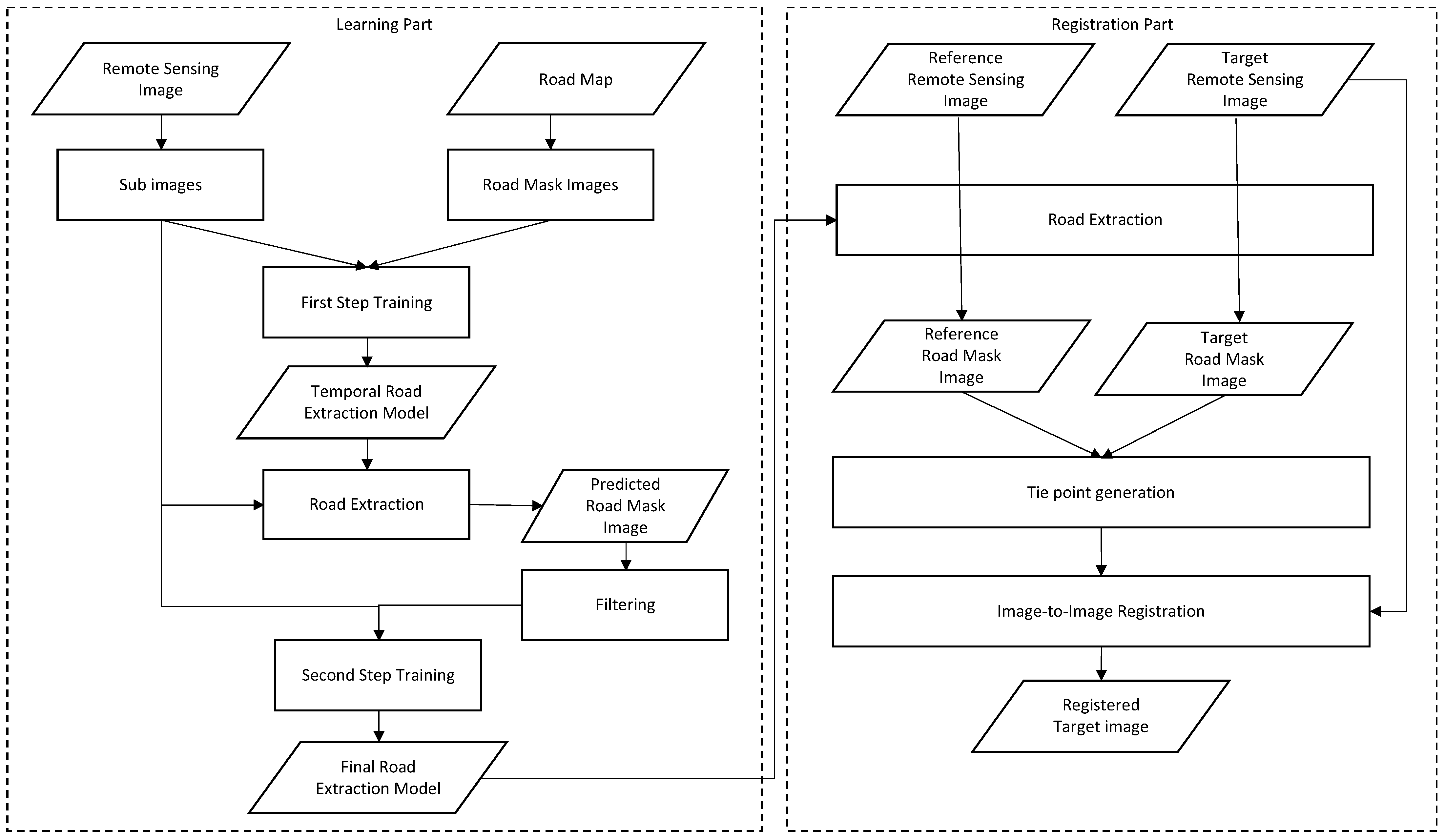
The proposed method consists of two parts: learning and registration. In the learning part, a road extraction model is created by deep learning using remote sensing images and corresponding road vector maps as training data. In the registration part, the road extraction model described above is first applied to two remote sensing images (reference and target) to generate road masks for each image. Then, the two resulting road mask images are divided into grids and the amount of misalignment at the tie points is calculated by applying template matching to each grid and registration between images is performed based on the amount of misalignment. There is no problem even if the registration images for the learning part and the reference/target remote sensing images for the registration part have different platforms and shooting times, but the spatial resolution should be consistent to some extent. In addition, although the learning must be performed before the registration, the road extraction model does not need to run the learning part for every registration because of its generalization performance. The overall process flow is shown in
Figure 1.
2.1.2. Road Extraction Model
The road extraction model of our method is based on U-Net [
37], a type of fully convolutional network (FCN) [
38] that is a deep learning network mainly used in image segmentation tasks. U-Net was proposed in 2015 for semantic segmentation of medical images, but is currently applied in various fields.
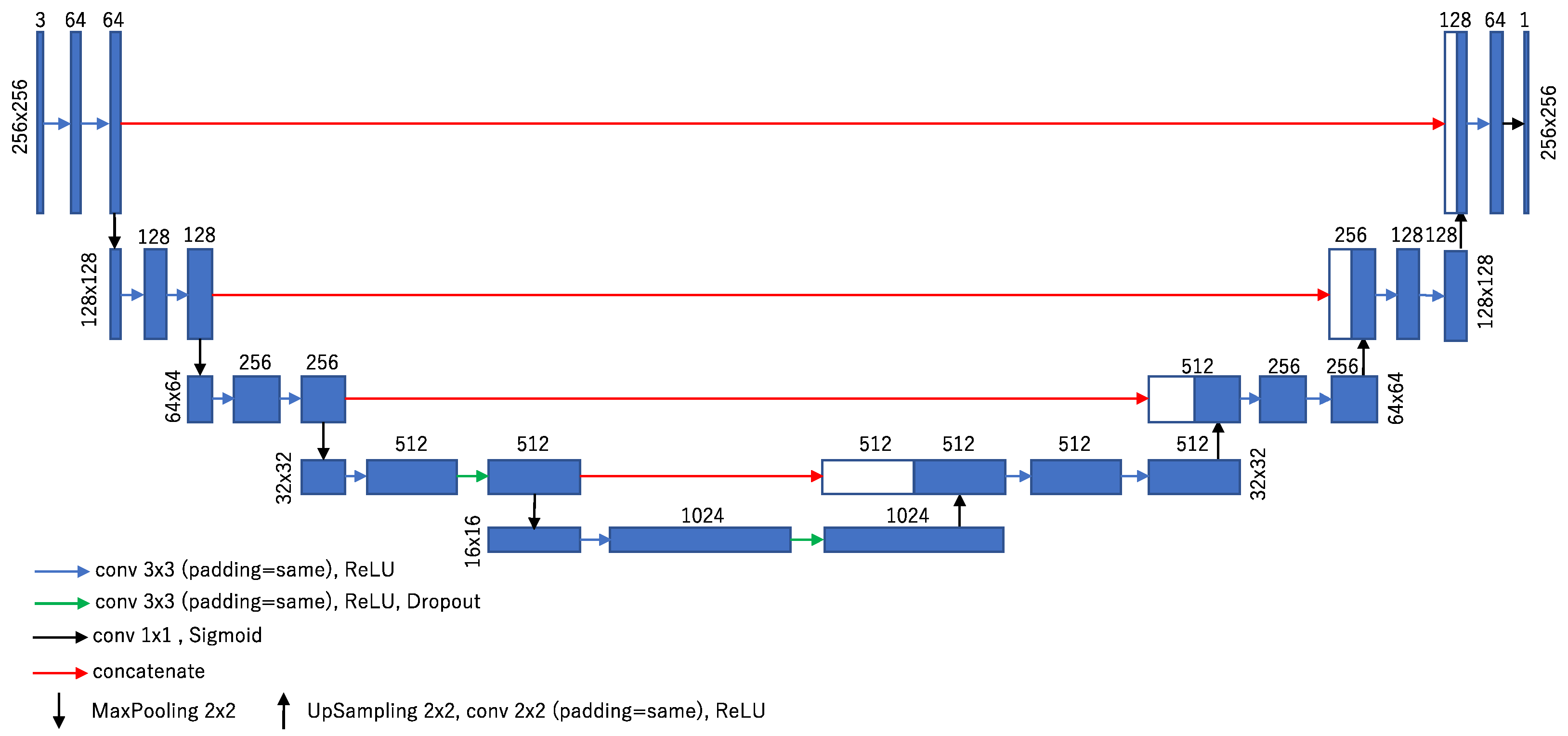
U-Net is characterized by its symmetrical encoder–decoder configuration: the encoder path repeats the 3 × 3 convolution and ReLU [
39] twice and down-sampling at the max pool is repeated four times. Each down-sampling halves the size of the feature map and doubles the number of channels, while the decoder pass repeats the up-sampling and 3 × 3 convolution four times. For each up-sampling, the size of the feature map is doubled and the number of channels is halved. Finally, a 1 × 1 convolution is performed to obtain per-pixel label predictions. A portion of the pre-down-sampled feature map in the encoder pass is combined with the corresponding feature map in the decoder pass as skip connections. This allows the recovery of object location information while retaining low-dimensional features in the decoder pass.
In this study, the following model based on the U-Net structure was adopted for road extraction. The network architecture of the model is shown in
Figure 2.
Input/output image values and size: The size of the input image of the model was 256 × 256. The number of input image channels was three RGB channels, assuming the use of aerial color photographs from the past. On the other hand, the output value of the model was the confidence value (0 to 1) for the estimation of the road area (i.e., the number of channels is 1). Here, a higher value for confidence means a higher accuracy for the road. The output image was the same size as the input image (256 × 256).
Application of zero padding: The original U-Net reduces the output image size during convolution and crops the center during skip connections, resulting in missing information around the patch image. Therefore, in the road extraction model, zero padding was applied so that the same size would be obtained before and after convolution. This process enables feature extraction near the edge of the patch image by increasing the number of convolutions for that edge.
Modification of activation function: Since the original U-Net was intended for segmentation, the activation function for the final layer is a pixel-wise soft-max function. On the other hand, the road extraction model in this study uses a pixel-wise sigmoid function as the activation function in the final layer, since it classifies two classes, road and non-road.
Addition of dropout: To suppress over-learning, dropouts [
40] are added at lower dimensional layers.
Loss function: The road extraction model of the proposed method classifies each pixel into two values, road or non-road, and generates a road mask image. Since the percentage of road pixels in the image is very small, the commonly used mean squared error (MSE), including the original U-Net, cannot be used as the loss function in the segmentation task. If MSE were used, the learning would be dominated by the non-road region, so the road region would not be output nearly as much. Therefore, the road extraction model of the proposed method differentiates the loss weights between road and non-road regions in order to be able to detect road regions. That is, in each pixel of the patch image, a relatively large penalty is imposed on any misinterpretation of roads by multiplying a weight greater than 1 for the loss when a road is misinterpreted as non-road, as expressed by:
where
k is the weight (>0),
m and
n are the number of road and non-road pixels in the training image, respectively, and
Cx and
Cy are the model outputs (confidence, 0–1) for road and non-road pixels in the training image, respectively.
Optimizers: Various optimizers have been proposed for finding the minimum loss function. The simplest and most basic algorithm is stochastic gradient descent (SGD), which has a constant learning rate and stable convergence results, which requires heuristically setting the optimal learning rate. Most of the currently proposed optimizers are extensions of SGD and one of the most widely used is adaptive moment estimation (Adam) [
41]. Adam achieves faster convergence by adjusting the learning rate according to the magnitude and sum of gradients of each parameter. On the other hand, since the variance of the learning rate becomes too large in the early stages of learning, resulting in convergence to a local solution, this is mitigated by a warm-up, which entails a low learning rate in the first few epochs [
42,
43,
44]. However, the hyperparameters of the warm-up need to be set heuristically. Therefore, the road extraction model of the proposed method uses RAdam [
45], an extension of Adam that incorporates a mechanism to automatically suppress the variance of the adaptive learning rate. The main feature of RAdam is that it does not require heuristic hyperparameter settings.
2.1.3. Training the Road Extraction Model
The training data for the road extraction model consisted of a set of remote sensing images (RGB color images) and road mask images (binary images) in a given area. Here, the road mask images were generated by raster transformation of a vector map of the road centerline, which had the same area, size and resolution as the remote sensing image. The width of the road centerline is constant regardless of the area and size of the road. Road boundary vector maps are also available, but unlike road centerline maps there is no open and widely maintained database for road boundary maps. For this reason, road centerline maps, which are readily available, were used.
However, road centerline maps that are freely available have many inconsistencies with remote sensing images due to differences in maintenance periods, registration gaps and ambiguities in acquisition criteria. In order to efficiently use such incomplete data without processing, the road extraction model was trained in two steps.
In the first step, the model was trained using the aforementioned U-Net and training data and in the second step the road mask was predicted and processed using the training data and the road extraction model learned in the first step and the road extraction model was trained again using this as training data. In image processing, morphological transformations (opening and closing) are performed to remove fine noise in road mask images, and road pixels below a certain confidence level are set to zero. By training the road extraction model in two steps, the quality of the training data and the accuracy of the model are raised incrementally.
In order to control over-learning, data augmentation is performed by flipping left and right, flipping up and down, changing gamma values and changing hue during model training. In addition to the output value of the loss function described above, the accuracy of the model was evaluated by the F1 score between pixels of the road mask image of the validation data randomly separated from the training data and the road mask image predicted from the remote sensing image of the validation data.
2.1.4. Road Mask Image Generation
Each road mask image is generated by cropping a 256 × 256 pixel chip image from the two remote sensing images used as reference and target and inputting them into the road extraction model. In order to suppress misclassification near the boundaries of the chip images, the images were cropped while sliding them so that the regions would overlap and the prediction results were assembled in the overlapping regions.
2.1.5. Tie Point Generation and Registration
Using the target and reference road mask images generated by the road extraction model from two remote sensing images, tie points for image-to-image registration are generated as follows. First, a sub-image is cropped from the target road mask image with a fixed size, centered on an arbitrary coordinate (cropping center coordinate). The size of the sub-image should be set at around 300 pixels square. Next, template matching is applied to the cropped sub-image and reference road mask image to estimate the amount of misalignment of the target road mask image in subpixel order (details given below). Then, the coordinates of the cropping center as well as the cropping center plus the amount of misalignment are recorded as a tie point. The above process is performed while sliding the cropping center coordinates so that the sub-images overlap and the tie points are obtained from the entire road mask image. However, since areas with few roads can generate wrong tie points, outliers are removed from the obtained tie points using random sample consensus (RANSAC) (details given below) [
46].
Finally, image-to-image registration is performed by feeding the obtained tie point data to a general geometric transformation method such as affine transformation.
- (1)
Tie point generation by template matching
The sum of absolute difference (SAD) [
47] is used to generate tie points by estimating the matching position of the target road mask image (sub-image) and the reference road mask image centered on an arbitrary coordinate:
where
dx and
dy are scanning positions,
T(x, y) and
I(x, y) are the brightness values of the target road mask sub-image and reference road mask image and
w and
h are the width and height of the template.
For SAD, the scanning position (
dx,
dy) that shows the smallest value is the matching point, but the position obtained is in pixel order. Therefore, in order to find the matching point in subpixel order, equiangular line fitting [
48] is performed, as shown in Equation (3):
where
S(0) is the minimum value of SAD,
S(−1) and S(1) are similarity values for two points near the origin in the
X- or
Y-axis direction and the value of
dsub is in the range of −0.5 to 0.5. By calculating
dsub for the
X-axis and
Y-axis and adding it to
dx and
dy, the match points of subpixel order can be obtained.
- (2)
Outlier removal by RANSAC
RANSAC is a method for extracting correct data from a set of data containing noise [
46]. The procedure is as follows:
Extract n points at random from all tie points in the reference and target images.
Find the coefficients of affine transformation based on the extracted n points.
Perform affine transformation on all tie points in the target image using the coefficients obtained in step 2 and calculate the error between obtained points and tie points in the reference image; tie points with errors within the threshold and their points are recorded as inliers.
Repeat steps 1 to 3 and adopt the set of inliers with the highest number of points as the final tie points.
2.2. Study Area and Data Used
2.2.1. Study Area
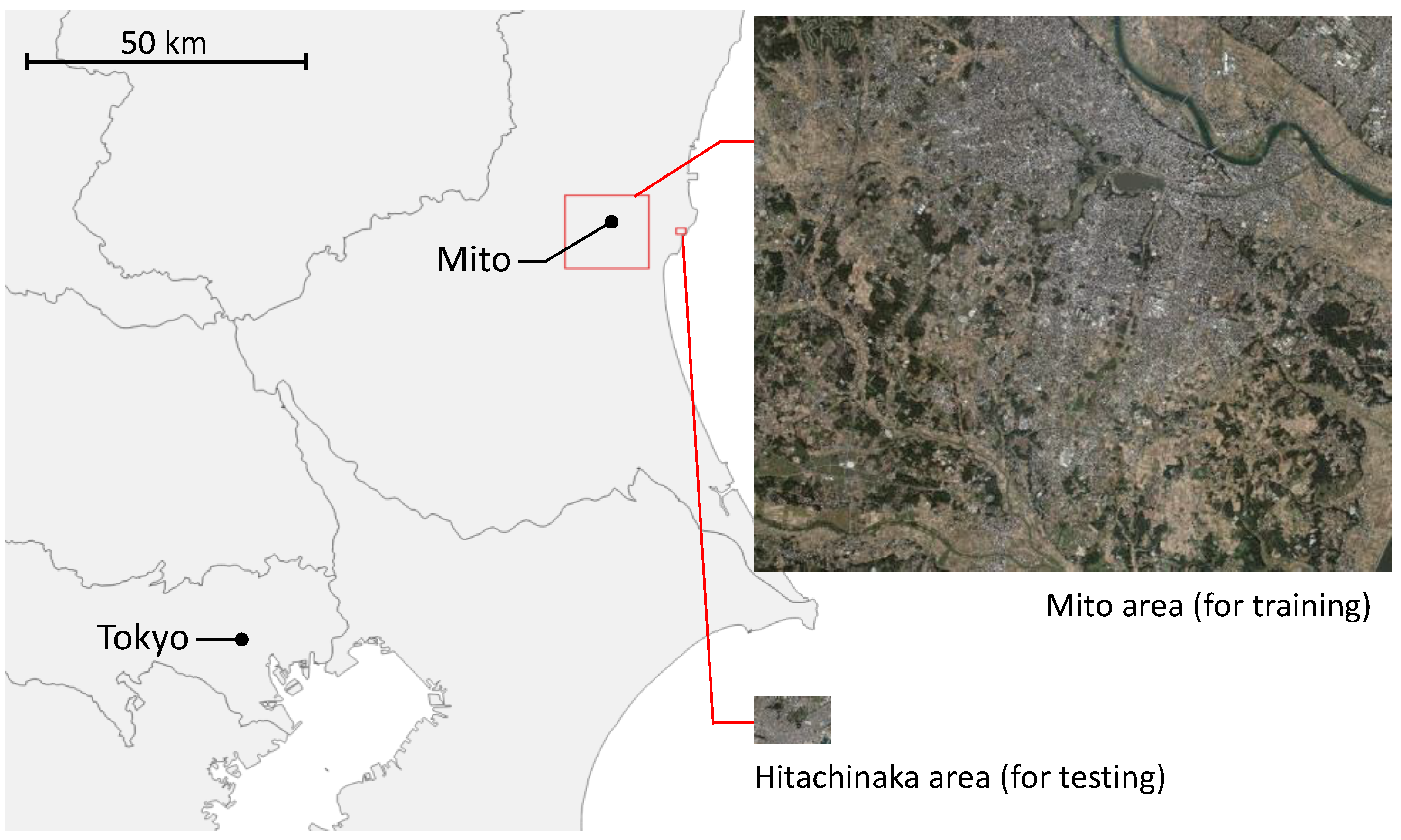
The study area was selected from parts of Mito City and Hitachinaka City in Ibaraki Prefecture, Japan (
Figure 3). The two cities are located next to each other, about 100 km northeast of Tokyo. The size of the study area is 202.637 square kilometers in Mito and 2.420 square kilometers in Hitachinaka. Both areas are predominantly residential, but also include commercial and industrial areas, farmland, forests, rivers and so on.
2.2.2. Remote Sensing Images
To validate the proposed method, aerial photographs from the Geospatial Information Authority of Japan (GSI) and images from the WorldView-3 (WV-3) satellite were prepared as remote sensing images (
Table 1). Aerial photographs acquired after 2007 (referred to as new-period aerial photos) were used for training and aerial photographs acquired from 1979 to 1983, 1984 to 1986 and after 2007 (referred to as old-period aerial photos 1 and 2 and new-period aerial photo, respectively) and WV-3 images acquired in 2019 were used for testing. The details of each dataset are described below.
- (1)
Aerial photographs
By-period aerial photographs published by GSI as GSI Tiles were used in this study. These comprise mosaicked and tile-distributed data for a fixed non-continuous period of time (5-10 years) starting in 1928. Each tile consists of map data in the Mercator projection system (EPSG 3857), divided into ranges corresponding to the zoom level, with the size of a single tile being a uniform 256 × 256 pixels. The file format is JPEG or PNG. The corresponding zoom level is defined within a range of 2 to 18 for each map type.
Old-period aerial photos were taken with analog film cameras and the maximum zoom level for a tile is 17. New-period aerial photos are taken with digital cameras and the maximum zoom level for a tile is 18. These images are geo-referenced orthoimages, but the degree of geometric distortion of buildings varies by location. The zoom level of the old- and new-period aerial photos used in this study was set to 17 to match the maximum zoom level of the old-period aerial photos. The pixel spacing at zoom level 17 is about 1.19 m.
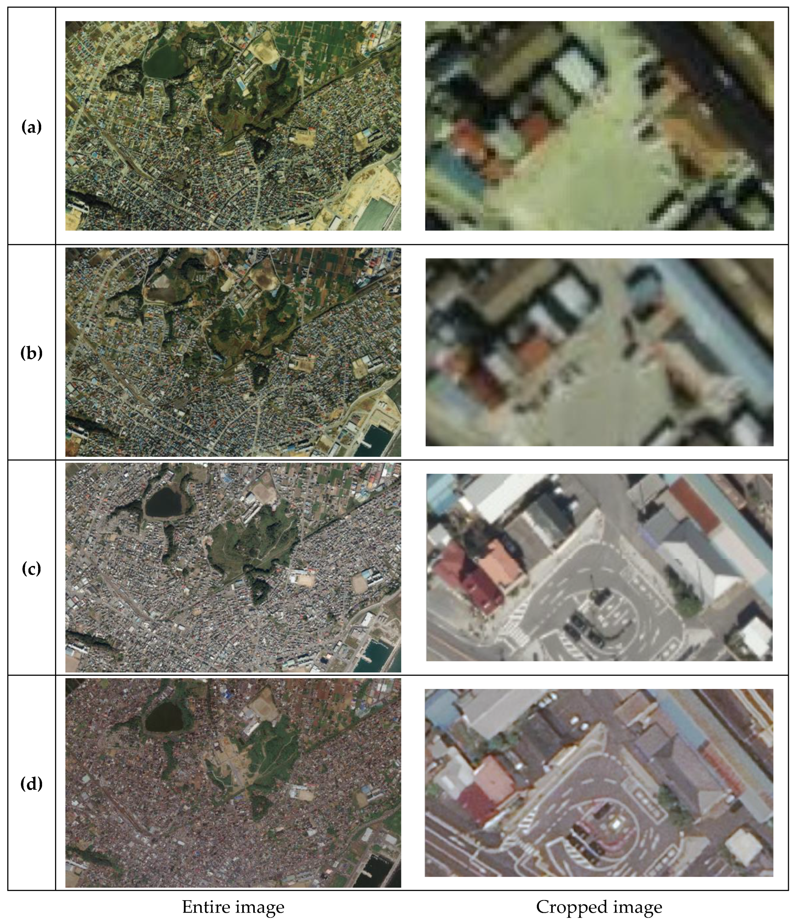
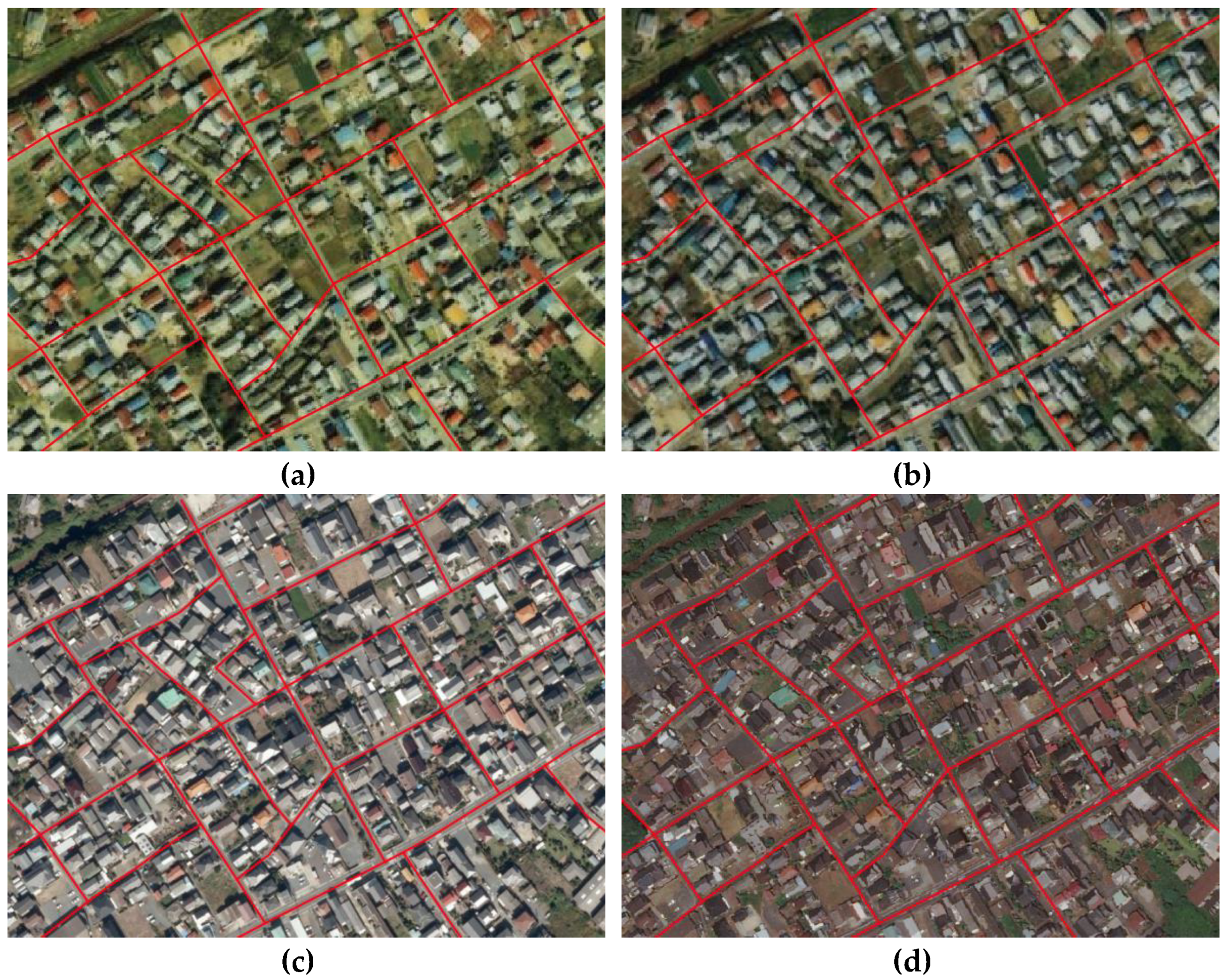
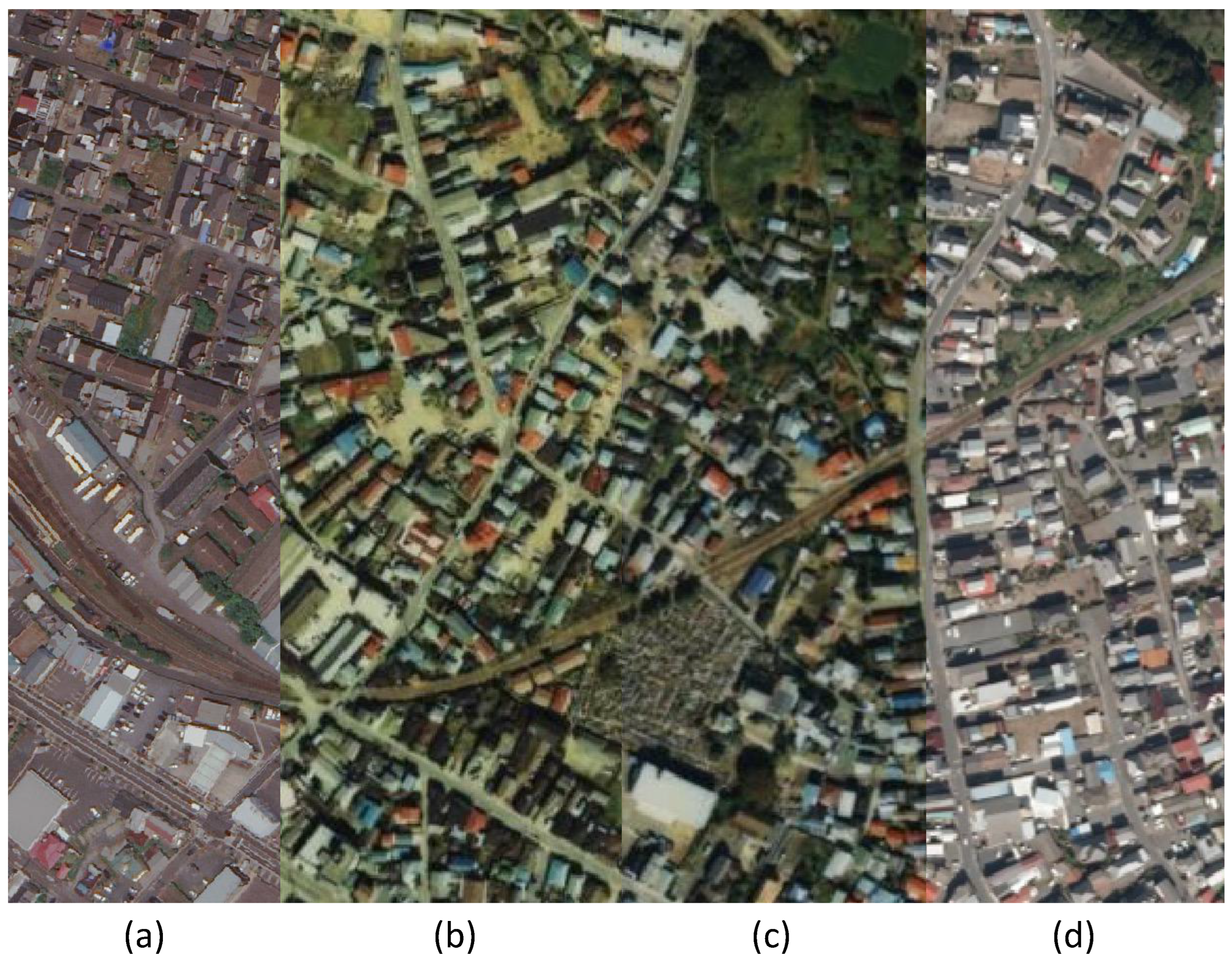
Figure 4 shows images of the old- and new-period aerial photos in the Hitachinaka area and images cropped as samples. As shown in the figure, the two types of photos have different tints and the resolution differs significantly even at the same zoom level. In particular, the boundaries of buildings, roads and other structures in the old-period aerial photos are ambiguous and, since the acquisition dates are more than 21 years before the new-period aerial photo and 33 years before the WV-3 image, many geographic features have changed. Therefore, it is not easy to manually obtain exact control points for registration.
- (2)
Optical satellite images
The WV-3 image used for evaluation was a pan-sharpened image with a resolution of 0.3 m from the AW3D ortho-ready image product by the Remote Sensing Technology Center of Japan (RESTEC) and NTT DATA Corp. The image was taken on 6 June 2019. The viewing angle is 25.5° and buildings have some geometric distortion. The entire WV-3 image of the Hitachinaka area and the image cropped as a sample are shown in
Figure 4. Compared to the previously described aerial photos, the color and resolution of these are similar to those of the new-period aerial photo. Since building boundaries and white lines on the road can be identified, it is relatively easy to manually acquire control points. However, care should be taken when using building boundaries as control points, since AW3D ortho-ready images are not corrected for distorted buildings.
2.2.3. Road Centerline Vector Data
In this study, we used road centerline vector data (gis_osm_roads_free.shp) [
49] published in shapefile format from the Open Street Map (OSM) project as training data. This road vector data comprises road centerlines, but arterial roads with two or more lanes may be represented by multiple lines. In many cases, narrow roads are omitted. Note that since OSM is a volunteer-based project, consistency in data preparation is not ensured.
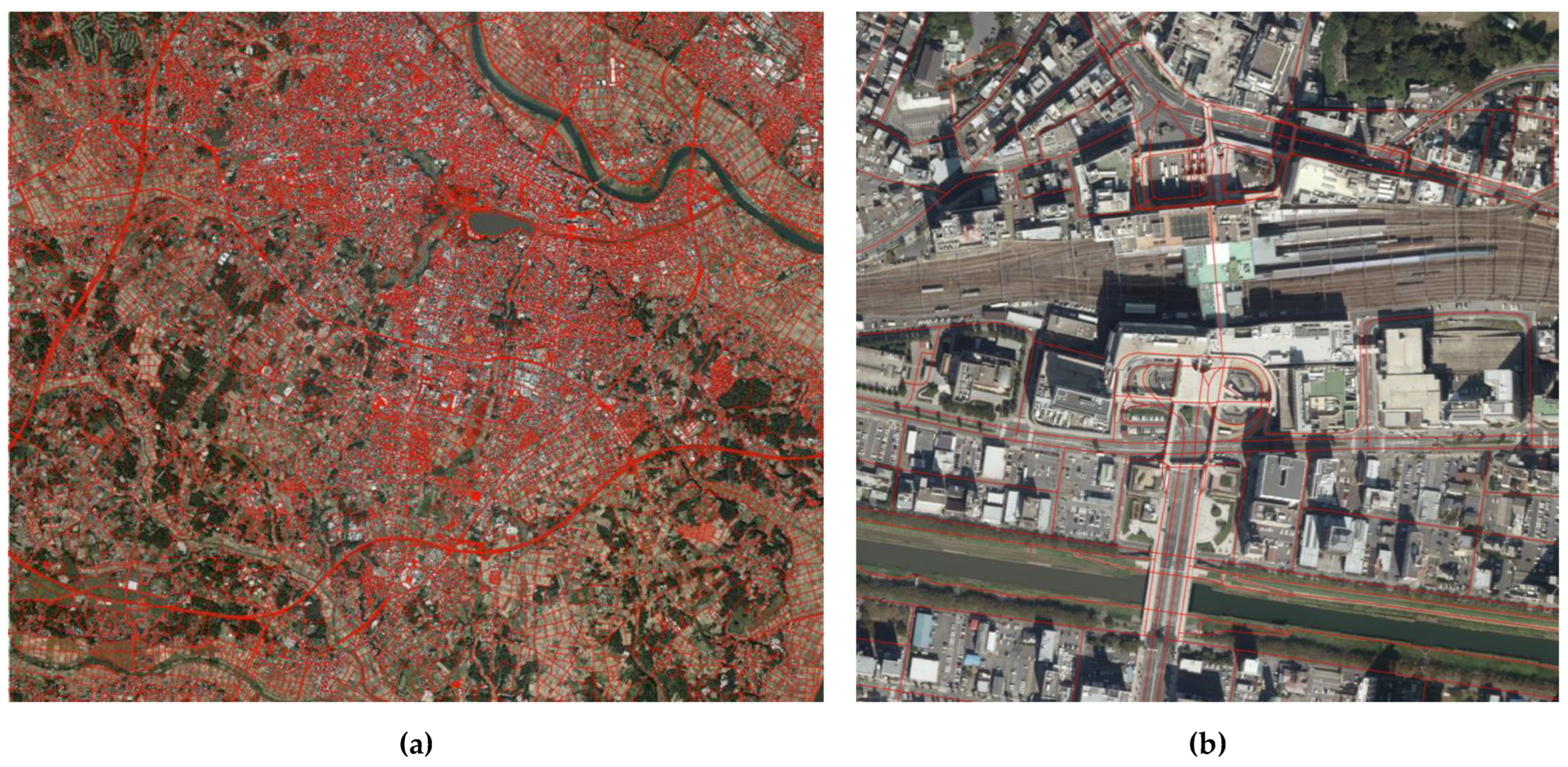
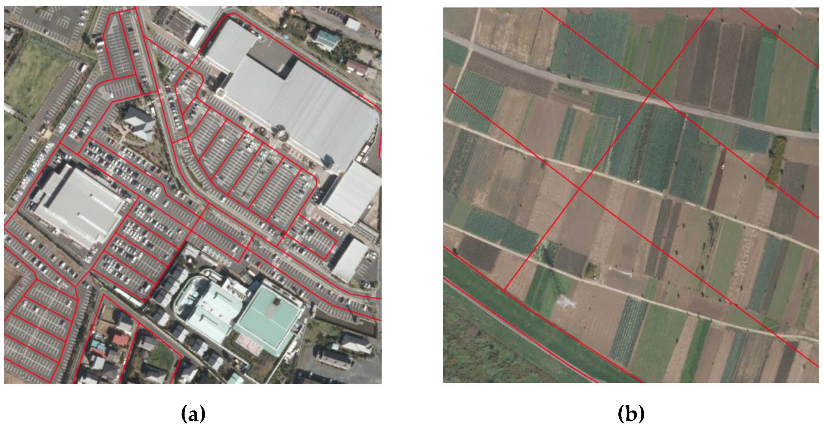
Figure 5 shows the OSM road centerline vector map overlaid on the new period aerial photo in the Mito area (an entire image and an enlarged image around the Mito Station).
2.3. Validation Methodology
2.3.1. Preliminary Evaluation of Location Accuracy of Training Data
Before applying the proposed method, the positional accuracy of the training data was evaluated in advance. First, the misalignment of the OSM road vector map was evaluated by superimposing it on the road edges included in the GSI road map, one of the GSI base maps. Then, the misalignment of the new-period aerial photo compared to the OSM road vector map was evaluated by superimposing them.
2.3.2. Preliminary Evaluation of Learning Methods and Parameters Used in Road Extraction Model
- (1)
Preliminary evaluation of loss function weight
To evaluate the effect of weight k of the loss function in Equation (1), learning was conducted for 20 cases, from k = 1.0 to k = 20.0, in steps of 1.0 and the results were compared. Here, for k = 1.0, the losses to detection errors on the road and the non-road are equivalent. In this comparative evaluation, RAdam was used as the optimizer in all cases, dropout was enabled and data augmentation was not performed.
Table 2 shows the learning conditions. The same conditions were used in the comparison and evaluations below.
- (2)
Comparison of optimizers
To evaluate the optimizers in learning, we applied three algorithms, SGD, Adam and RAdam and compared the results. The hyperparameters of each algorithm are given in
Table 3; for Adam, the hyperparameter values from the original paper [
41] were adopted.
In this comparative evaluation, weight k of the loss function was set to 10.0 for all optimizers, dropout was enabled and no data augmentation was performed.
- (3)
Evaluation of the effectiveness of dropout
Dropout is considered effective for suppressing overlearning. Therefore, to evaluate the effectiveness of dropout in this study, learning was conducted in two patterns, with and without dropout, and the results were compared. In both cases, weight k of the loss function was set to 10.0, the optimizer was RAdam and no data augmentation was performed in the evaluation.
- (4)
Evaluation of the effectiveness of data augmentation
Data augmentation is also considered effective for suppressing overlearning. To evaluate its effectiveness in this study, learning was conducted in two patterns, with and without data augmentation, and the results were compared. In the case of data augmentation, we randomly applied left-to-right and up-and-down flipping and gamma value and hue changes to the input data (a new-period aerial photo and a patch image pair of road mask images) during training. In all evaluations, the loss function weight k was set to 10.0, the optimizer was RAdam and dropout was enabled.
2.3.3. Application and Evaluation of the Proposed Method
Using the learning methods and parameters that were found to be valid in
Section 2.3.2, the road extraction model was trained. In the Hitachinaka area, roads were extracted by inputting the new-period aerial photo that was not used for training and the old-period aerial photos and WV-3 images for testing into the road extraction model and the results were qualitatively evaluated by visual inspection.
Tie points were generated and registered from the WV-3 image, old-period aerial photos 1 and 2 and the new-period aerial photo using the proposed method and the results were visually and qualitatively evaluated.
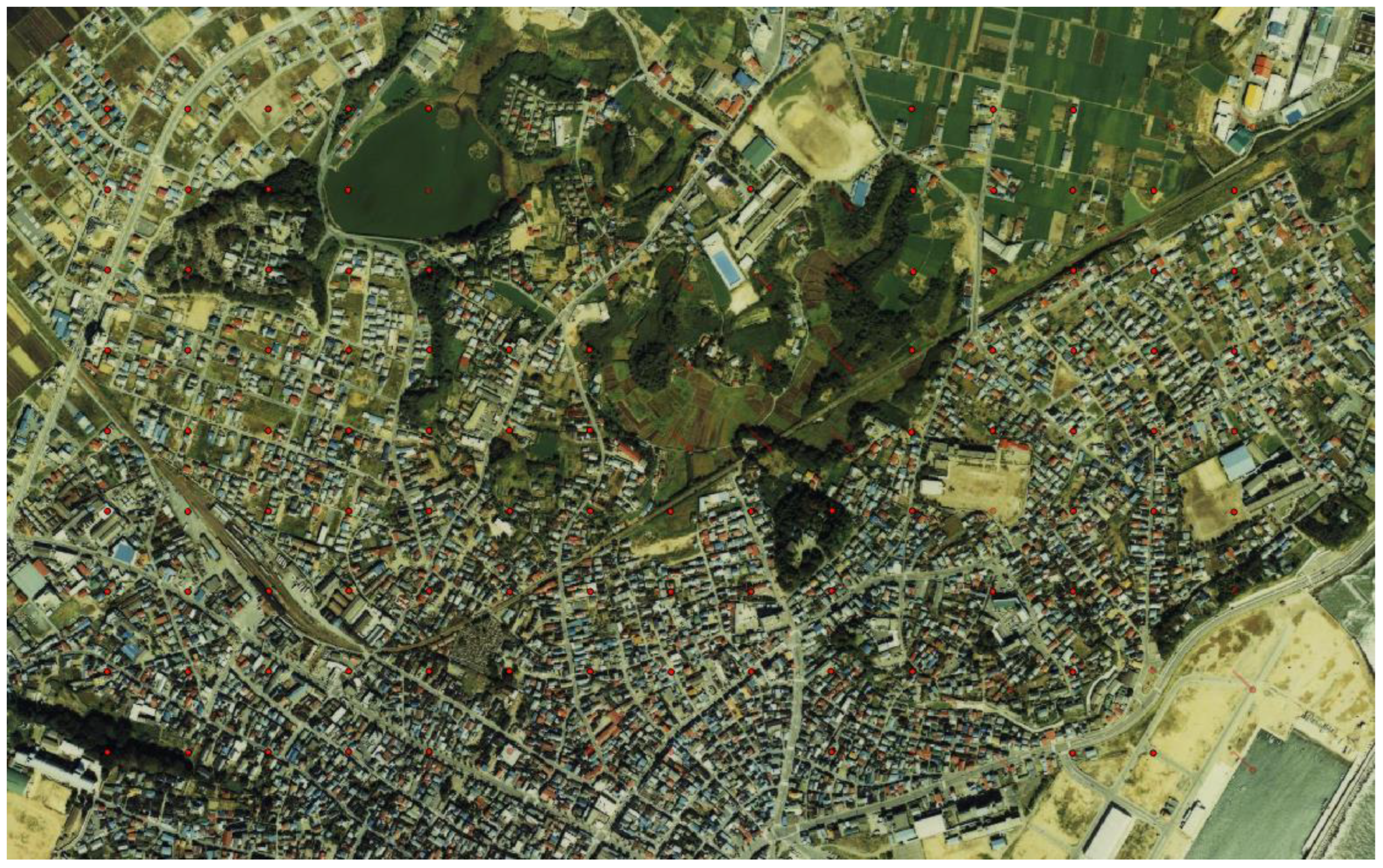
Using the proposed method, tie points were generated and registered using a combination of loss function weights (8 cases; 2 steps from 6 to 20) and sub-image sizes for template matching (21 cases; 20-pixel steps from 100 to 500) and the accuracy was compared, with accuracy defined as the root mean square difference (RMSD) (pixels) between ground control points (GCPs), for evaluation of the reference image and registered target image. The GCP set did not include the tie points used in the registration, but consisted of multiple points manually obtained from the entire test area (Figure 10).
To compare the accuracy of the proposed method, tie point generation and registration were performed using the following methods:
One-step U-Net: This is an optional version of the proposed method that uses only one step to train the road extraction model.
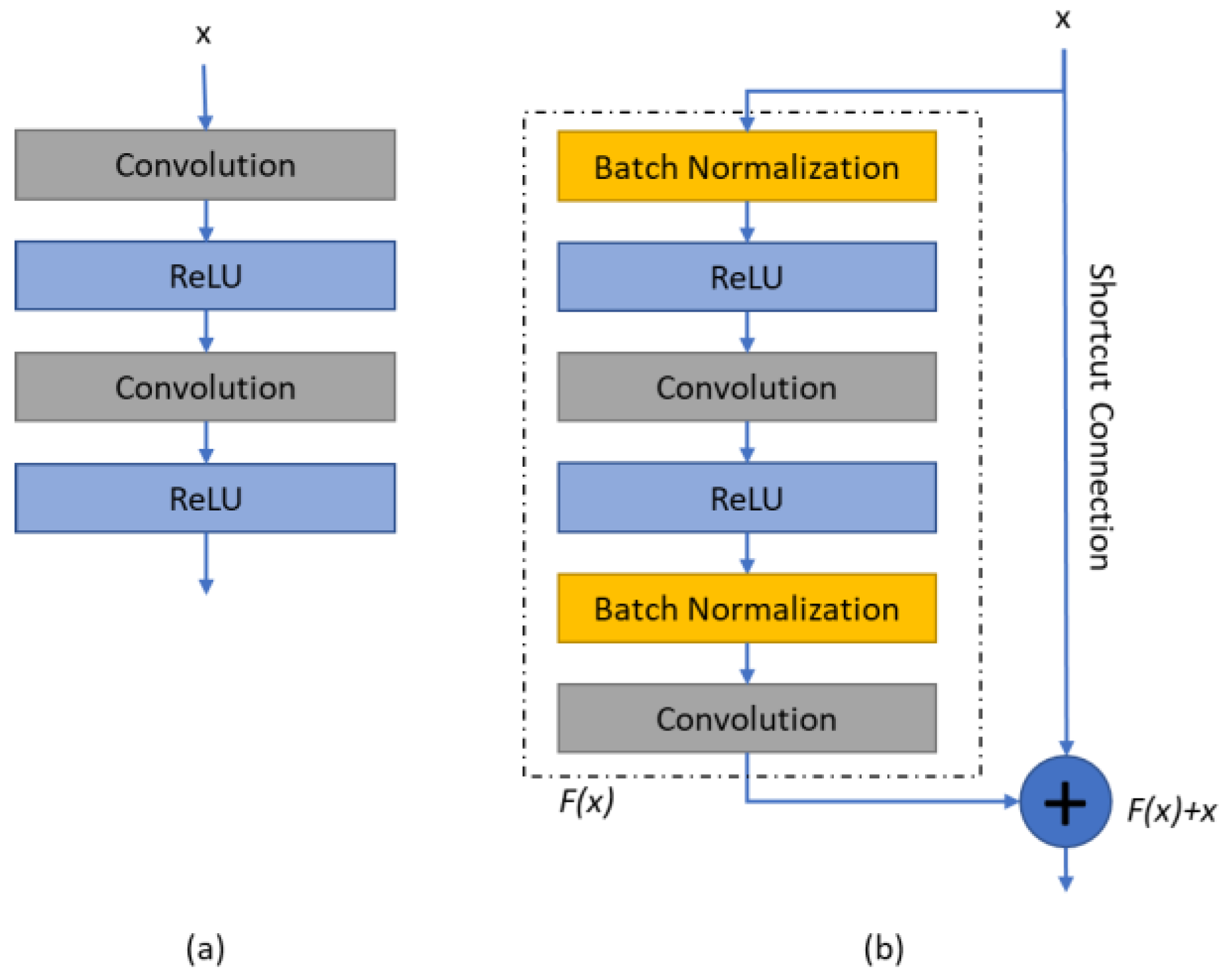
One-step ResU-Net: This is another optional version of the proposed method in which a residual U-Net (ResU-Net) [
50] with only one step is used instead of U-Net. ResU-Net, like ResNet [
51], is expected to prevent accuracy loss due to gradient loss and divergence (
Figure 6).
Phase-only correlation (POC): This is a method that performs Fourier transform on sub-images cut from target and reference images and uses their phase spectra to match images [
22]. Compared to the method that simply matches brightness values, POC enables highly accurate matching because the steep solution peaks can be more closely measured. In the proposed method, POC can be used instead of template matching (SAD) for tie point generation.
Area-based method: This method generates tie points by directly applying template matching or POC to the image itself (not the road mask). The process after generating tie points is the same as the proposed method.
Feature-based method (CFOG): The channel features of oriented gradients (CFOG) method [
29] constructs pixel-by-pixel feature descriptors from images using one-cell HOG blocks and performs fast local feature point matching using fast Fourier transform (FFT). Compared to conventional feature-based methods, this method supports multimodal image registration by constructing feature descriptors at high density.
For the proposed (road-based) method, the loss function weight was set to 10. To compare the methods, the average of the results (RMSD between GCPs) for different sub-image sizes (21 sizes, from 100 × 100 to 500 × 500 pixels in 20-pixel steps) during template matching was used as the accuracy.
3. Results
3.1. Preliminary Evaluation of Location Accuracy of Training Data
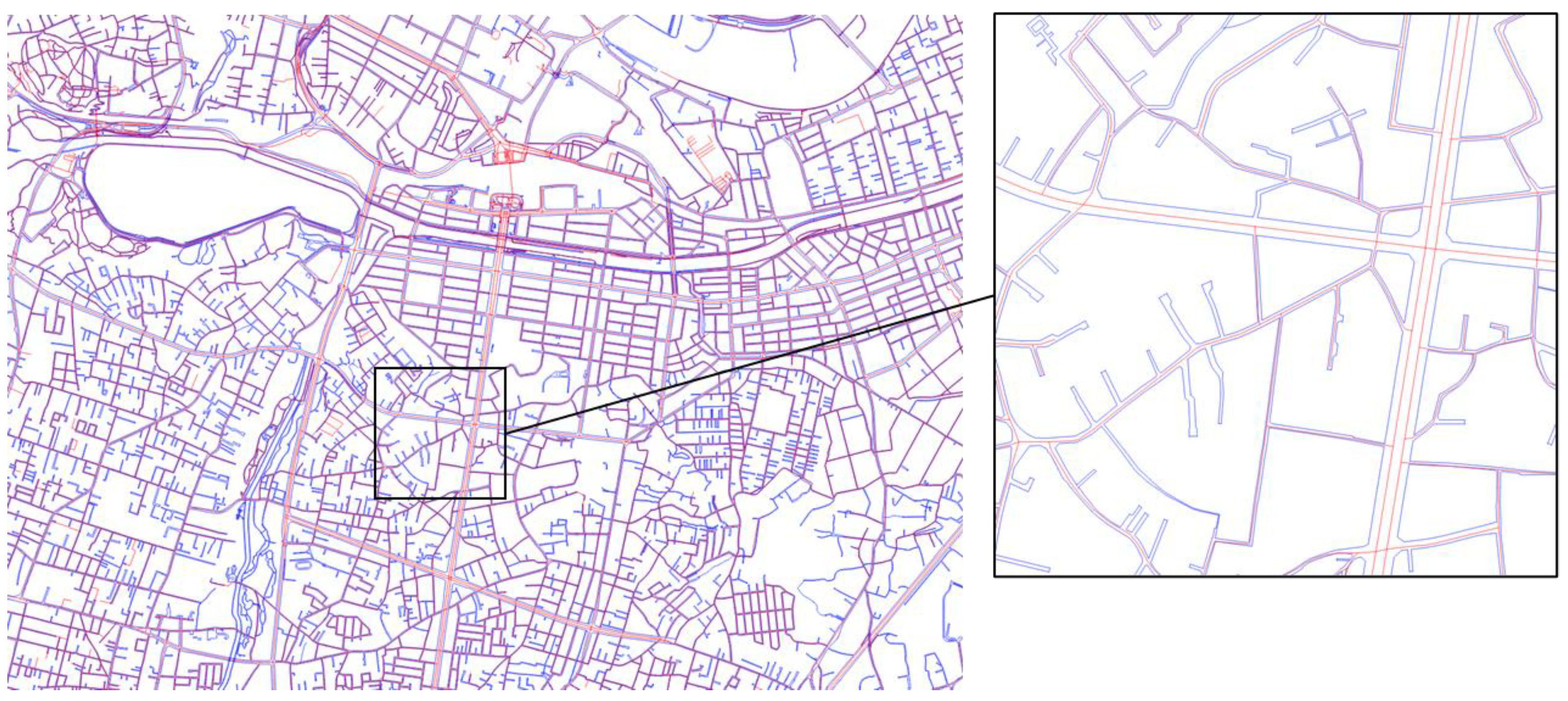
Figure 7 shows the superposition of the OSM and GSI maps. It can be seen that the road centerline of the OSM road vector map is superimposed on the center of the road edge in the GSI road map. However, in many cases, some of the roads included in GSI road maps are not included in OSM road vector maps, especially narrow roads in small residential areas. The total road length in the study area was approximately 3527 km on the GSI road map, while it was 2822 km on the OSM road vector map. Thus, the OSM map has good location accuracy, but the maintenance rate is not very high.
Figure 8c shows the superimposition of the OSM road vector map and the new-period aerial photo; it can be seen that their locations are generally consistent. However, similar to the results of the comparison with the GSI road map, there are many instances where the OSM map does not include some of the roads visible in the new-period aerial photo. On the other hand, as shown in
Figure 9a, there are also instances where an excessive number of roads is obtained. In addition, as shown in
Figure 9b, there are several instances where the roads in the OSM map do not match the roads in the new-period aerial photo, mainly in suburban areas. These are considered to be due to either human error or roads that were redeveloped after the OSM road vector map was created.
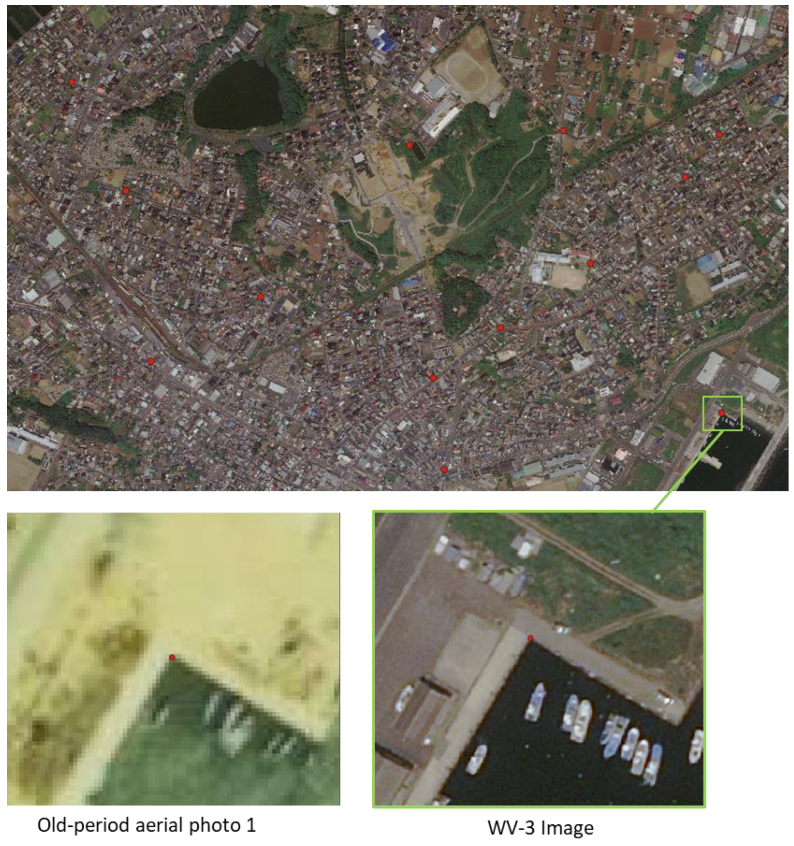
Figure 8 shows the superposition of the OSM road vector map, old-period aerial photos 1 and 2, new-period aerial photo and WV-3 image. All of the remote sensing images show slight deviations, especially in the old-period aerial photos. The residuals were calculated by acquiring several visible common points (GCPs) of the four images and the results show that the RMSD of old-period aerial photos 1 and 2 and the new-period aerial photo is 4.166, 5.166 and 0.951 pixels, respectively, based on the WV-3 image. The placement of GCPs and an enlarged view of one of them are shown in
Figure 10.
3.2. Preliminary Evaluation of Learning Methods and Parameters Used in the Road Extraction Model
- (1)
Preliminary evaluation of loss function weight
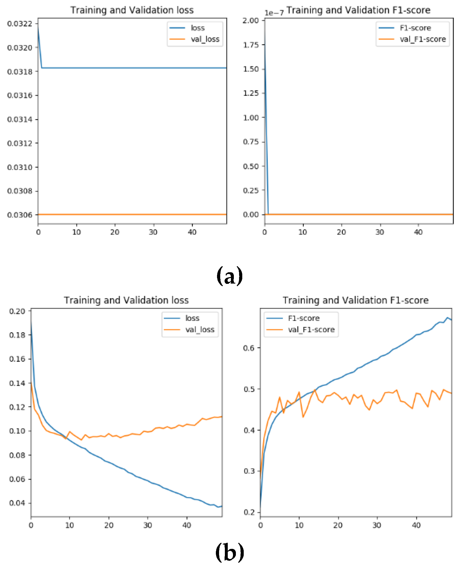
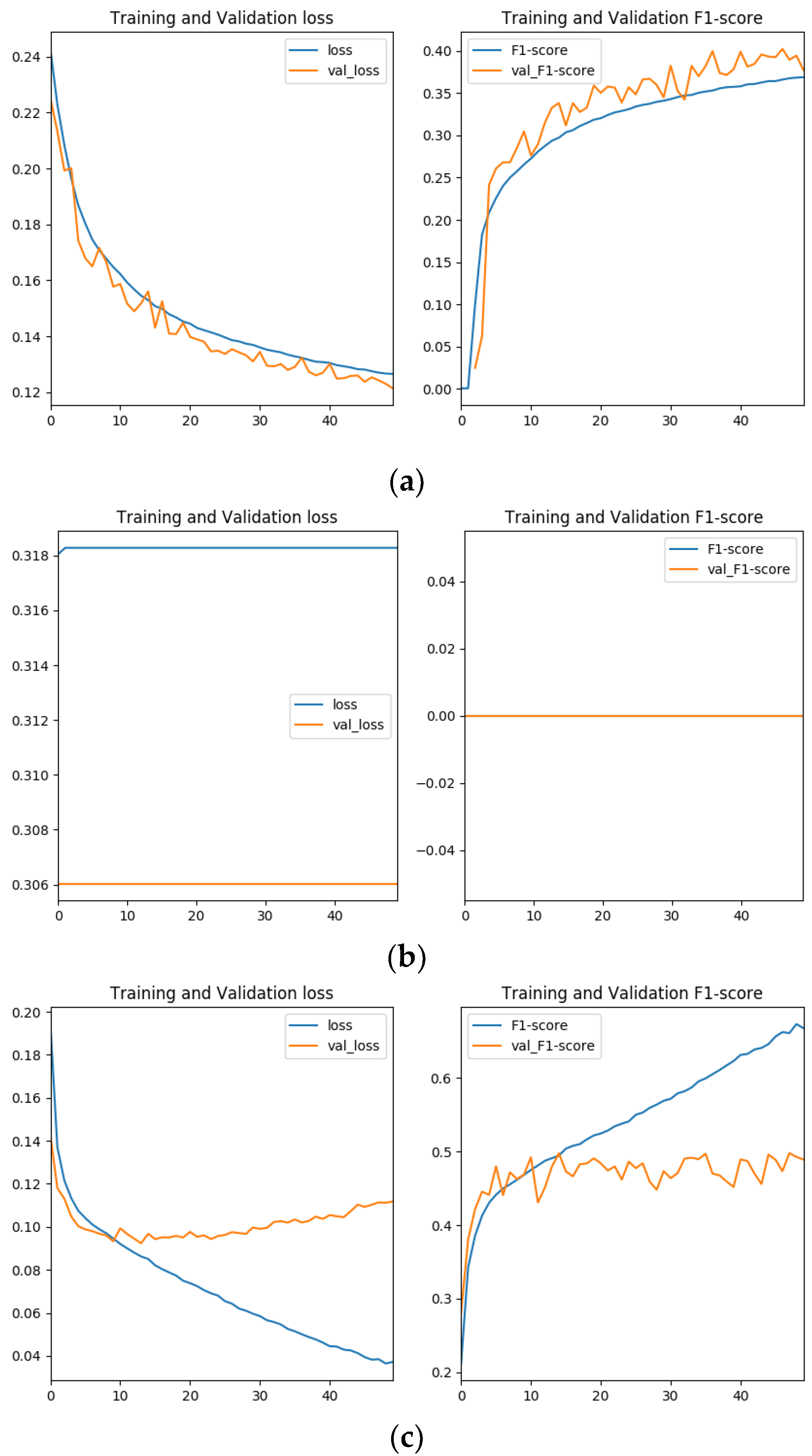
Figure 11 shows the loss and accuracy (F1 score) during learning when k values of 1.0 and 10.0 are given as the loss function weights. As shown in the figure, when k = 1.0, with the same weight for roads and non-roads, learning did not progress and no roads were detected, but when k = 10.0, with 10 times the weight given to roads, roads were properly detected and the transition of loss and accuracy between training and validation data gradually moved toward convergence according to epoch.
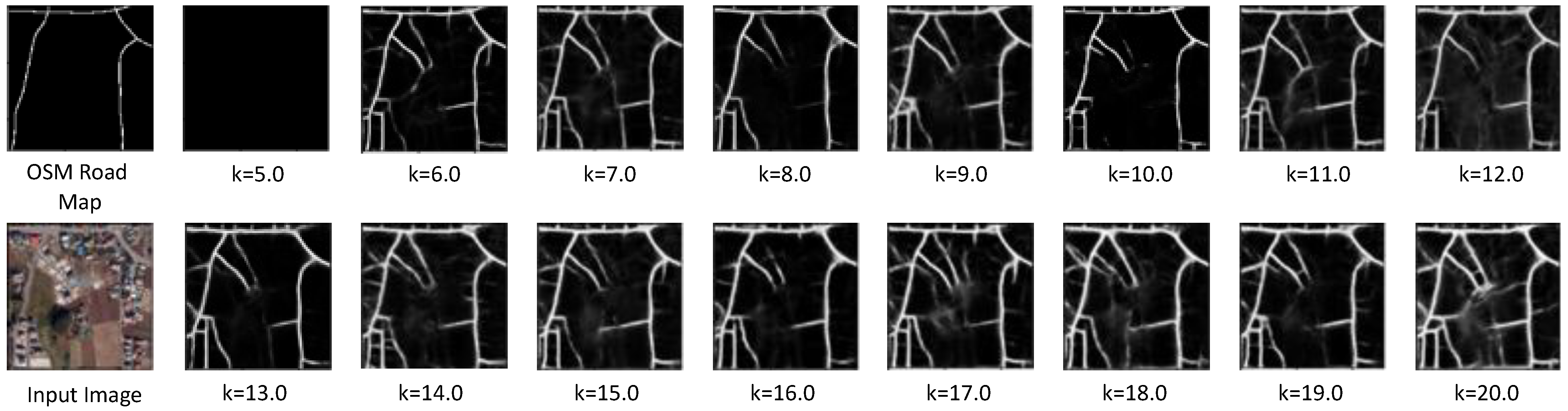
Figure 12 shows examples of the prediction results of the model when the loss function weight was given by steps of 1.0 from k = 1.0 to 20.0. The results indicate that learning progressed when k = 6.0 and above. It was also confirmed that, as k increased, the extracted roads became thicker and even the narrowest roads were extracted. It is also noteworthy that roads were extracted without being affected by the shadows of buildings.
- (2)
Comparison of optimizers
Figure 13 shows the learning loss and accuracy when SGD, Adam and RAdam were used as optimizers. It can be seen that the learning speed of RAdam was more than five times faster than that of SGD; SGD had a loss of 0.127 and an F1 score of 0.369 at 50 epochs and RAdam had a loss of 0.093 and an F1 score of 0.468 at 10 epochs, although RAdam showed a larger discrepancy between training and validation loss after 10 epochs. Note that Adam fell into a local solution in the early epoch and did not progress properly in learning.
- (3)
Evaluation of the effectiveness of dropout
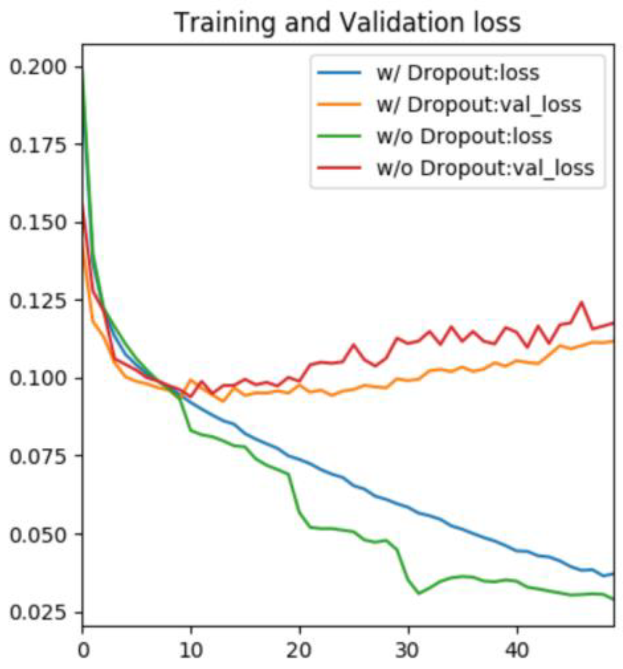
Figure 14 shows the training and validation losses during learning with and without dropout. In both cases, a deviation between the two losses occurred around epoch 10, confirming overlearning. However, it can be confirmed that the gap between the two losses became smaller after epoch 10 when dropout was added to the network.
- (4)
Evaluation of the effectiveness of data augmentation
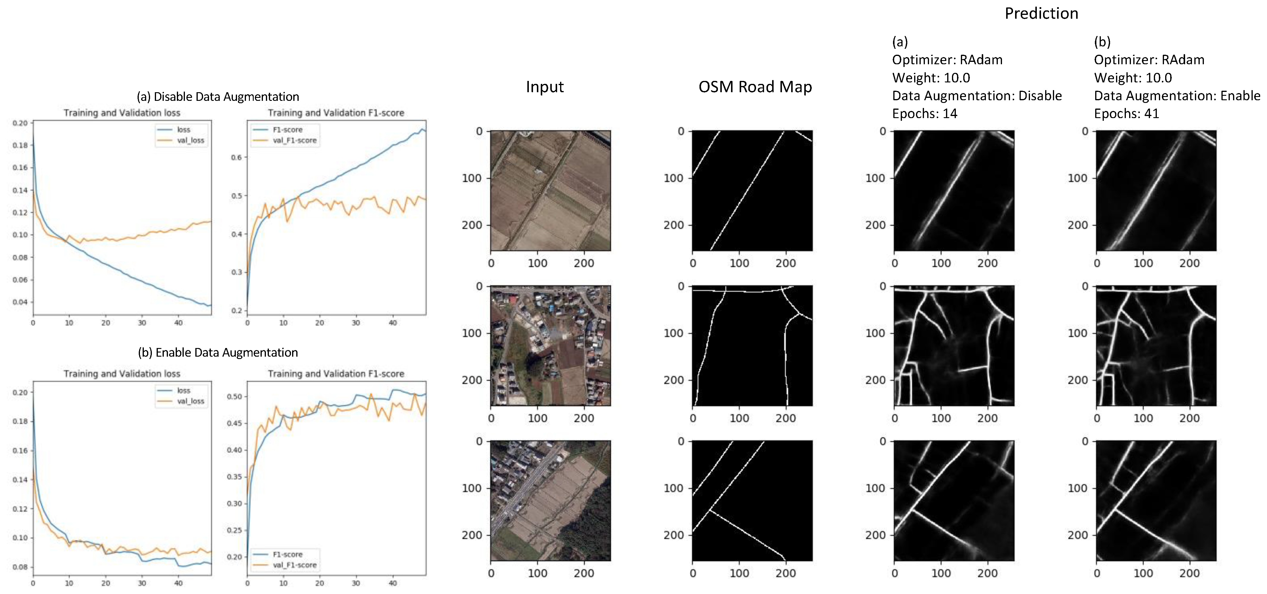
The left panel of
Figure 15 shows loss and accuracy during learning with and without data augmentation. It can be seen that the deviation between training and validation losses, which occurred after epoch 10 in RAdam, was reduced by data augmentation, indicating that over-learning was suppressed. The right side of
Figure 15 provides examples of the prediction results of the model at the epoch with the smallest validation loss, showing the input new-period aerial photo, the roads visually extracted from the input image and the prediction results without and with data augmentation. It can be seen that the results with data augmentation include narrow roads that were missed by visual interpretation.
3.3. Application and Validation of the Proposed Method
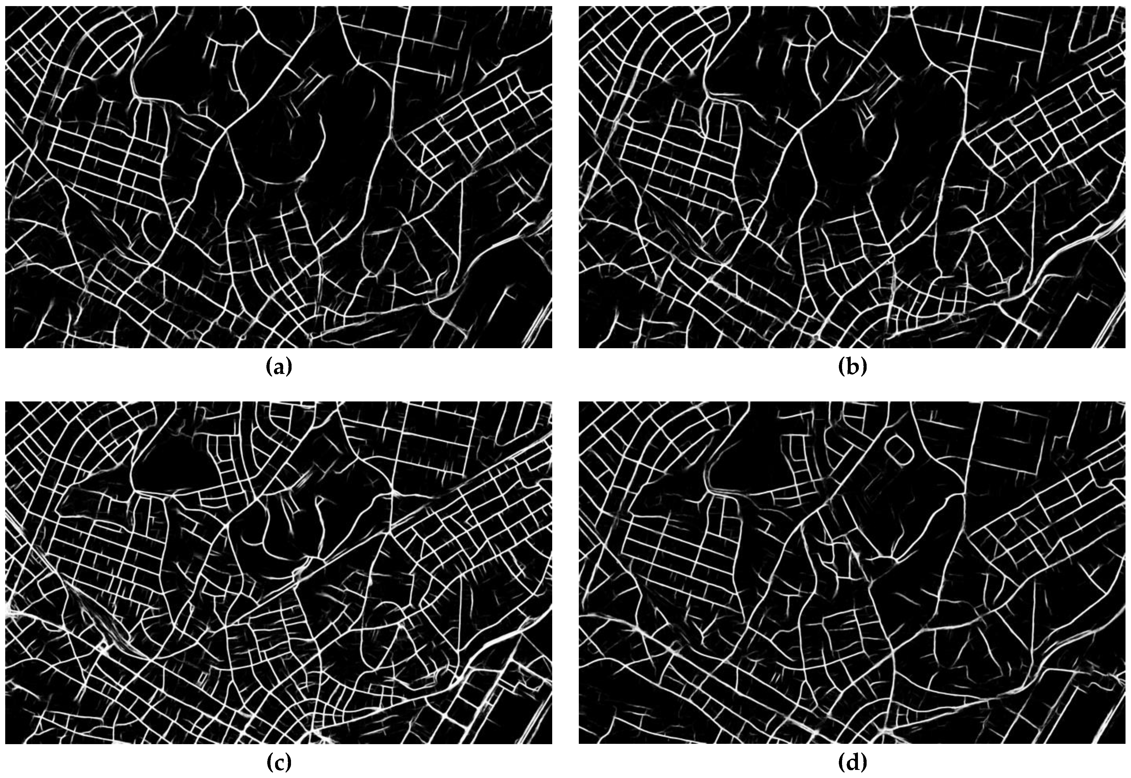
Figure 16 shows the predicted images produced by the road extraction model using the new-period aerial photo, WV-3 image and old-period aerial photos of the test area as input. The predicted images have the same resolution as the respective input images and the model’s prediction accuracy of roads is given as a value (0–1). Here, the closer the prediction accuracy is to 1, the higher the confidence that the road is in fact a road. It can be seen in the figure that the overall road network is generally consistent across images. This indicates that the road network in this area did not change significantly in the nearly 40 years from the oldest aerial photograph to the newest WV-3 image. Some areas where the differences between images are somewhat large, such as near the upper center, are mainly due to the development of new residential areas. Road extraction is somewhat dependent on image quality, and narrower roads were also extracted in the clearest new-period aerial photo.
Figure 17 shows the tie points and residuals generated by the proposed method for the WV-3 image and old-period aerial photo 1, mapped on the latter. Many tie points, shown by dark red dots, are adopted ones, while other tie points, shown by transparent red dots, are those excluded by RANSAC. Most of the excluded points are situated around the vegetation area in the upper center and the harbor area in the lower right.
Figure 18 shows a mosaic of the reference image (WV-3) and the registered images (old-period aerial photos 1 and 2 and the new-period aerial photo). In the mosaicked image, the boundaries between images are consistent and no misalignment can be seen, indicating that the registration by the method worked as expected.
Table 4 lists the mean, standard deviation and minimum RMSD of inter-GCP residuals for different loss function weights (k) for sub-image size (W) from 100 to 500 at 20-pixel steps using old-period aerial photos 1 and 2 and the new-period aerial photo as target images. A smaller RMSD value indicates a smaller registration error and a smaller standard deviation of RMSD indicates a smaller error variance between weights. As shown in the table, the variation of registration error with weight is small. On the other hand, there is a large difference in registration error depending on the image used, with smaller errors for the newer images, probably due to higher consistency in the road network and higher image quality. The table also shows the mean RMSD for W ≤ 280 and W ≥ 300, indicating that the sub-image size has no significant effect on the registration error.
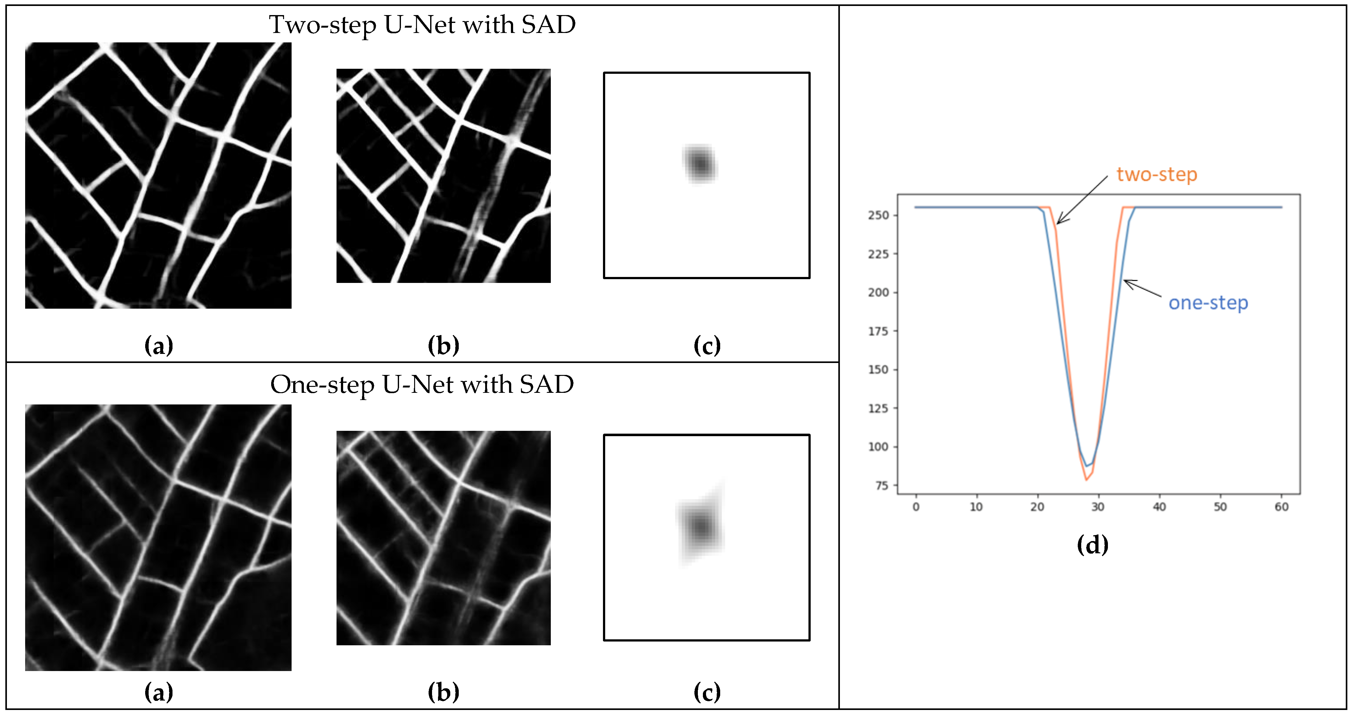
Table 5 shows the mean and standard deviation of RMSD of inter-GCP residuals by applying different methods (four road-based methods based on the proposed method, two area-based methods based on SAD and POC, CFOG and no registration) to old-period aerial photos 1 and 2 and the new-period aerial photo as target images. The table shows that the proposed road-based methods have higher mean accuracy than the area-based methods and CFOG, except for the old-period aerial photo by method 2 (two-step U-Net with POC), indicating that registration is possible at the subpixel level. The reason for the larger error seen in the old-period aerial photo by method 2 is likely due to the poor performance of POC when there are large differences between the two road mask images. In the comparison of road-based methods, method 1 (two-step U-Net with SAD) had the highest accuracy.
Figure 19 shows a comparison of the template matching similarity map and curve between two-step U-Net with SAD and one-step U-Net with SAD (methods 1 and 2, respectively, in
Table 5) using the road mask image from the WV-3 image as the reference and the one from old-period aerial photo 1 as the target. Because the contrast of the road mask image was increased and the noise was reduced by using the two-step method, a steeper similarity curve can be seen. This may be the main reason why the two-step method showed higher registration accuracy.
4. Discussion
The proposed method uses a deep learning road extraction model to generate road mask images from two images to be used for registration between images and then performs template matching to detect misalignment on a grid basis. To evaluate whether the proposed method can be applied for registration between remote sensing images that were taken at different times and are of different quality, we applied it to multitemporal aerial photographs and high-resolution satellite images with different tints, resolution and shooting times.
When the reference image was a satellite image (WV-3 image) and the target image was an aerial photograph, the misalignment before registration was 4.166 pixels, 5.146 pixels and 0.951 pixels for RMSD in the order of the older aerial photograph. Registration using the proposed method improved the RMSD to 0.847, 0.524 and 0.463 pixels, which are all less than one pixel off the RMSD. The more recent the image, the smaller the RMSD value. This was because the closer the shooting times of the target and reference images were, the more stable the processing was, because there were fewer differences in the road network and the image quality was sharper in the newer images.
We then investigated the impact of different loss function weights during road extraction model training and different sizes of sub-images that served as input for template matching during tie point generation. It was confirmed that the effect of changing these parameters on the results was less than 0.1 pixel, which is negligible for practical use. In particular, the loss function weight had a significant impact on the road extraction results, but the impact was not significant for the end-to-end process with weights greater than 6. This indicates that the proposed method is robust to parameters during training.
The comparison between the proposed method and other methods shows that the accuracy of the proposed method is significantly higher than that of common area-based methods (template matching and POC) and feature-based methods (CFOG), indicating that this method is superior for registration of images with different time periods and color tones. Compared with an optional version of the proposed method, in which the training step of the road extraction model is reduced to one step, the originally proposed two-step method, with two training steps, has superior performance in accuracy for all images and the improvement in accuracy is particularly significant for the oldest images. When comparing the similarity maps obtained during template matching, the two-step method also produced steeper peaks. This shows the effectiveness of the two-step method. In addition, in the comparison between ResU-Net and U-Net in the one-step method, the latter outperformed the former on accuracy for all images, indicating that accuracy can be achieved even with a simple network architecture.
The difference between the brightness-domain template matching (SAD) and frequency-domain POC method was minimal for the most recent aerial photographs, but SAD was superior for the older aerial photographs. The difference was particularly large for the oldest aerial photograph, with an RMSD value for SAD of 0.847 pixels compared to 2.638 pixels for POC.
In generating the road extraction model, the OSM road vector map, which is widely available in many areas, was used as the training data. A comparison between the OSM road vector map and the GSI base map and new-period aerial photo showed that the OSM map had sufficient positional accuracy, but in some cases roads in small residential areas and newly developed suburban areas were not included, or roads were not positioned correctly. However, even if some errors were included, they were shown to have little effect on the accuracy of the road extraction model, as long as the data were predominantly of acceptable quality. This indicates the robustness of the road extraction model. Since the road extraction model was constructed using only the new-period aerial photo, its accuracy and robustness may be further improved by including data with image characteristics similar to those of the old-period aerial photos and the WV-3 image as training data.
In building the road extraction model, we evaluated the loss function, optimizer, dropout and data augmentation. For the loss function, it was shown that by assigning weights to roads, learning progresses and converges appropriately and roads can be extracted. For the optimizer, it was shown that learning proceeds several times faster with RAdam than with SGD. This is thought to occur because RAdam dynamically adjusts the learning rate, resulting in more efficient parameter updating and learning progress. On the other hand, RAdam also tended to overlearn early, which could be suppressed by using dropout and data augmentation. Data augmentation can also extract narrow roads that are not included in the training data, which improves generalization performance.
The proposed method is based on the assumption that the road network has not changed much between the two images to be registered, so it may not be accurate or applicable under conditions where this is not the case. For example, in this evaluation, a large discrepancy was identified in some grids with large proportions of vegetation. This was due to the absence or small number of roads in these grids. However, the methods that apply template matching directly to brightness images were affected by seasonal and secular changes in vegetation and showed larger discrepancies than the proposed method. Therefore, the proposed method, which uses road mask images, is robust to temporal variations in vegetation and is also superior in that it does not need to consider aligning the seasons of the two images. This method is also robust to the shadows of buildings, which can be an error factor in area-based and feature-based methods, because it uses deep learning to extract roads without much influence from shadows. This robustness of the proposed method against vegetation and building shadows shows its superiority. Even if there are no roads in some grids, the proposed method is still applicable because outliers are excluded from those grids and misalignment is estimated by interpolation from surrounding grids.
5. Conclusions
In this study, we propose an image-to-image registration method that can be robustly and accurately applied to remote sensing images with different sensor characteristics and acquisition dates, especially for monitoring over time in urban areas. The proposed method does not directly generate tie points by calculating the misalignment between two remote sensing images, but rather extracts roads from each image using a deep learning model, applies template matching to estimate the amount of misalignment and generates tie points. The evaluation results show that the proposed method is robust to differences in the sensor characteristics, acquisition time, resolution and color tone of two remote sensing images, as well as to temporal variations in vegetation and the effects of building shadows. The accuracy of this method was higher than that of the main conventional area-based and feature-based methods, especially for older images with large differences in color tone and texture. The amount of error after registration was also shown to be smaller than the pixel spacing of the remote sensing images used, regardless of the time of year they were taken.
These results were obtained with a road extraction model trained on images from a single area, single time period and single platform, demonstrating the high versatility of the model. In further development, the performance will be improved and stabilized by using images from different areas, time periods and platforms for training. For cases where the road structure has changed significantly between the two images, or for non-urban areas with sparse roads, the proposed method is difficult to apply in principle and a different approach should be chosen, but the method is expected to contribute to the analyses of short- and long-term changes using remote sensing data in many urban areas.
Author Contributions
Conceptualization, S.H. and H.T.; methodology, S.H.; software, S.H.; validation, S.H.; formal analysis, S.H.; investigation, S.H.; resources, H.T.; data curation, S.H.; writing—original draft preparation, S.H.; writing—review and editing, H.T.; visualization, S.H.; supervision, H.T.; project administration, H.T.; funding acquisition, H.T. All authors have read and agreed to the published version of the manuscript.
Funding
This research was partially funded by the Environmental Research and Technology Development Fund of the Environmental Restoration and Conservation Agency of Japan (JPMEERF20S11811).
Data Availability Statement
Not applicable.
Acknowledgments
We used a WorldView-3 image, provided as an AW3D orthoimage which is copyrighted by Maxar Technologies, Inc. and NTT DATA Corp. and was prepared by the Remote Sensing Technology Center of Japan (RESTEC). We also used road vector data maintained by the OpenStreetMap project with the help of OSM contributors.
Conflicts of Interest
The authors declare no conflict of interest. The funders had no role in the design of the study; in the collection, analyses, or interpretation of data; in the writing of the manuscript, or in the decision to publish the results.
References
- Wu, Q.; Li, H.-Q.; Wang, R.-S.; Paulussen, J.; He, Y.; Wang, M.; Wang, B.-H.; Wang, Z. Monitoring and Predicting Land Use Change in Beijing Using Remote Sensing and GIS. Landsc. Urban Plan. 2006, 78, 322–333. [Google Scholar] [CrossRef]
- Yagoub, M.M. Monitoring of Urban Growth of a Desert City through Remote Sensing: Al-Ain, UAE, between 1976 and 2000. Int. J. Remote Sens. 2004, 25, 1063–1076. [Google Scholar] [CrossRef]
- Hegazy, I.R.; Kaloop, M.R. Monitoring Urban Growth and Land Use Change Detection with GIS and Remote Sensing Techniques in Daqahlia Governorate Egypt. Int. J. Sustain. Built Environ. 2015, 4, 117–124. [Google Scholar] [CrossRef] [Green Version]
- Dell’Acqua, F.; Gamba, P. Remote Sensing and Earthquake Damage Assessment: Experiences, Limits, and Perspectives. Proc. IEEE 2012, 100, 2876–2890. [Google Scholar] [CrossRef]
- Ceresola, S.; Fusiello, A.; Bicego, M.; Belussi, A.; Murino, V. Automatic Updating of Urban Vector Maps. In Proceedings of the Image Analysis and Processing—ICIAP 2005, Cagliari, Italy, 6–8 September 2005; Springer: Berlin/Heidelberg, Germany, 2005; pp. 1133–1139. [Google Scholar]
- Bouziani, M.; Goïta, K.; He, D.-C. Automatic Change Detection of Buildings in Urban Environment from Very High Spatial Resolution Images Using Existing Geodatabase and Prior Knowledge. ISPRS J. Photogramm. Remote Sens. 2010, 65, 143–153. [Google Scholar] [CrossRef]
- Matikainen, L.; Hyyppä, J.; Ahokas, E.; Markelin, L.; Kaartinen, H. Automatic Detection of Buildings and Changes in Buildings for Updating of Maps. Remote Sens. 2010, 2, 1217–1248. [Google Scholar] [CrossRef] [Green Version]
- Albayrak, U.; Canbaz, M.; Albayrak, G. A Rapid Seismic Risk Assessment Method for Existing Building Stock in Urban Areas. Procedia Eng. 2015, 118, 1242–1249. [Google Scholar] [CrossRef] [Green Version]
- Mangalathu, S.; Sun, H.; Nweke, C.C.; Yi, Z.; Burton, H.V. Classifying Earthquake Damage to Buildings Using Machine Learning. Earthq. Spectra 2020, 36, 183–208. [Google Scholar] [CrossRef]
- Du, Y.; Teillet, P.M.; Cihlar, J. Radiometric Normalization of Multitemporal High-Resolution Satellite Images with Quality Control for Land Cover Change Detection. Remote Sens. Environ. 2002, 82, 123–134. [Google Scholar] [CrossRef]
- Lu, D.; Mausel, P.; Brondízio, E.; Moran, E. Change Detection Techniques. Int. J. Remote Sens. 2004, 25, 2365–2401. [Google Scholar] [CrossRef]
- Chen, G.; Hay, G.J.; Carvalho, L.M.T.; Wulder, M.A. Object-Based Change Detection. Int. J. Remote Sens. 2012, 33, 4434–4457. [Google Scholar] [CrossRef]
- Hussain, M.; Chen, D.; Cheng, A.; Wei, H.; Stanley, D. Change Detection from Remotely Sensed Images: From Pixel-Based to Object-Based Approaches. ISPRS J. Photogramm. Remote Sens. 2013, 80, 91–106. [Google Scholar] [CrossRef]
- Tang, Y.; Huang, X.; Zhang, L. Fault-Tolerant Building Change Detection From Urban High-Resolution Remote Sensing Imagery. IEEE Geosci. Remote Sens. Lett. 2013, 10, 1060–1064. [Google Scholar] [CrossRef]
- Wang, H.; Ellis, E.C. Image Misregistration Error in Change Measurements. Photogramm. Eng. Remote Sens. 2005, 71, 1037–1044. [Google Scholar] [CrossRef] [Green Version]
- Shi, W.; Hao, M. Analysis of Spatial Distribution Pattern of Change-Detection Error Caused by Misregistration. Int. J. Remote Sens. 2013, 34, 6883–6897. [Google Scholar] [CrossRef]
- Chen, G.; Zhao, K.; Powers, R. Assessment of the Image Misregistration Effects on Object-Based Change Detection. ISPRS J. Photogramm. Remote Sens. 2014, 87, 19–27. [Google Scholar] [CrossRef]
- Thévenaz, P.; Ruttimann, U.E.; Unser, M. A Pyramid Approach to Subpixel Registration Based on Intensity. IEEE Trans. Image Process. 1998, 7, 27–41. [Google Scholar] [CrossRef] [Green Version]
- Sarvaiya, J.N.; Patnaik, S.; Bombaywala, S. Image Registration by Template Matching Using Normalized Cross-Correlation. In Proceedings of the 2009 International Conference on Advances in Computing, Control, and Telecommunication Technologies, Trivandrum, India, 28–29 December 2009; pp. 819–822. [Google Scholar]
- Kim, J.; Fessler, J.A. Intensity-Based Image Registration Using Robust Correlation Coefficients. IEEE Trans. Med. Imaging 2004, 23, 1430–1444. [Google Scholar] [CrossRef] [Green Version]
- Cole-Rhodes, A.A.; Johnson, K.L.; LeMoigne, J.; Zavorin, I. Multiresolution Registration of Remote Sensing Imagery by Optimization of Mutual Information Using a Stochastic Gradient. IEEE Trans. Image Process. 2003, 12, 1495–1511. [Google Scholar] [CrossRef]
- Takita, K.; Aoki, T.; Sasaki, Y.; Higuchi, T.; Kobayashi, K. High-Accuracy Subpixel Image Registration Based on Phase-Only Correlation. IEICE TRANSACTIONS Fundam. Electron. Commun. Comput. Sci. 2003, 86, 1925–1934. [Google Scholar]
- Nagashima, S.; Aoki, T.; Higuchi, T.; Kobayashi, K. A Subpixel Image Matching Technique Using Phase-Only Correlation. In Proceedings of the 2006 International Symposium on Intelligent Signal Processing and Communications, Yonago, Japan, 12–15 December 2006; pp. 701–704. [Google Scholar]
- Miura, M.; Sakai, S.; Aoyama, S.; Ishii, J.; Ito, K.; Aoki, T. High-Accuracy Image Matching Using Phase-Only Correlation and Its Application. In Proceedings of the 2012 Proceedings of SICE Annual Conference (SICE), Akita, Japan, 20–23 August 2012; pp. 307–312. [Google Scholar]
- Takenaka, H.; Sakashita, T.; Higuchi, A.; Nakajima, T. Geolocation Correction for Geostationary Satellite Observations by a Phase-Only Correlation Method Using a Visible Channel. Remote Sens. 2020, 12, 2472. [Google Scholar] [CrossRef]
- Rasmy, L.; Sebari, I.; Ettarid, M. Automatic Sub-Pixel Co-Registration of Remote Sensing Images Using Phase Correlation and Harris Detector. Remote Sens. 2021, 13, 2314. [Google Scholar] [CrossRef]
- Yu, L.; Zhang, D.; Holden, E.-J. A Fast and Fully Automatic Registration Approach Based on Point Features for Multi-Source Remote-Sensing Images. Comput. Geosci. 2008, 34, 838–848. [Google Scholar] [CrossRef]
- Patel, M.I.; Thakar, V.K.; Shah, S.K. Image Registration of Satellite Images with Varying Illumination Level Using HOG Descriptor Based SURF. Procedia Comput. Sci. 2016, 93, 382–388. [Google Scholar] [CrossRef] [Green Version]
- Ye, Y.; Bruzzone, L.; Shan, J.; Bovolo, F.; Zhu, Q. Fast and Robust Matching for Multimodal Remote Sensing Image Registration. IEEE Trans. Geosci. Remote Sens. 2019, 57, 9059–9070. [Google Scholar] [CrossRef] [Green Version]
- Lowe, D.G. Object Recognition from Local Scale-Invariant Features. In Proceedings of the Seventh IEEE International Conference on Computer Vision, Corfu, Greece, 20–27 September 1999; Volume 2, pp. 1150–1157. [Google Scholar]
- Dalal, N.; Triggs, B. Histograms of Oriented Gradients for Human Detection. In Proceedings of the 2005 IEEE Computer Society Conference on Computer Vision and Pattern Recognition (CVPR’05), San Diego, CA, USA, 20–26 June 2005; Volume 1, pp. 886–893. [Google Scholar]
- Hasan, M.; Jia, X.; Robles-Kelly, A.; Zhou, J.; Pickering, M.R. Multi-Spectral Remote Sensing Image Registration via Spatial Relationship Analysis on Sift Keypoints. In Proceedings of the 2010 IEEE International Geoscience and Remote Sensing Symposium, Honolulu, HI, USA, 25–30 July 2010; pp. 1011–1014. [Google Scholar]
- Plummer, M.; Stow, D.; Storey, E.; Coulter, L.; Zamora, N.; Loerch, A. Reducing Shadow Effects on the Co-Registration of Aerial Image Pairs. Photogramm. Eng. Remote Sens. 2020, 86, 177–186. [Google Scholar] [CrossRef]
- Long, T.; Jiao, W.; He, G.; Wang, W. Automatic Line Segment Registration Using Gaussian Mixture Model and Expectation-Maximization Algorithm. IEEE J. Sel. Top. Appl. Earth Obs. Remote Sens. 2014, 7, 1688–1699. [Google Scholar] [CrossRef]
- Yu, Z.; Prinet, V.; Pan, C.; Chen, P. A Novel Two-Steps Strategy for Automatic GIS-Image Registration. In Proceedings of the 2004 International Conference on Image Processing, ICIP ’04, Singapore, 24–27 October 2004; Volume 3, pp. 1711–1714. [Google Scholar]
- Qu, Z.; Gao, Y.; Wang, P.; Wang, P.; Chen, X.; Luo, F.; Shen, Z. Straight-Line Based Image Registration in Hough Parameter Space. In Proceedings of the 2011 International Workshop on Multi-Platform/Multi-Sensor Remote Sensing and Mapping, Xiamen, China, 10–12 January 2011. [Google Scholar]
- Ronneberger, O.; Fischer, P.; Brox, T. U-Net: Convolutional Networks for Biomedical Image Segmentation. arXiv 2015, arXiv:1505.04597. [Google Scholar]
- Long, J.; Shelhamer, E.; Darrell, T. Fully Convolutional Networks for Semantic Segmentation. In Proceedings of the 2015 IEEE Conference on Computer Vision and Pattern Recognition (CVPR), Boston, MA, USA, 7–12 June 2015; pp. 3431–3440. [Google Scholar]
- Nair, V.; Hinton, G.E. Rectified Linear Units Improve Restricted Boltzmann Machines. In Proceedings of the Proceedings of the 27th International Conference on International Conference on Machine Learning, Haifa, Israel, 21–24 June 2010; Omnipress: Madison, WI, USA, 2010; pp. 807–814. [Google Scholar]
- Srivastava, N.; Hinton, G.; Krizhevsky, A.; Sutskever, I.; Salakhutdinov, R. Dropout: A Simple Way to Prevent Neural Networks from Overfitting. J. Mach. Learn. Res. 2014, 15, 1929–1958. [Google Scholar]
- Kingma, D.P.; Ba, J. Adam: A Method for Stochastic Optimization. arXiv 2014, arXiv:1412.6980. [Google Scholar]
- Vaswani, A.; Shazeer, N.; Parmar, N.; Uszkoreit, J.; Jones, L.; Gomez, A.N.; Kaiser, Ł.U.; Polosukhin, I. Attention Is All You Need. In Proceedings of the Advances in Neural Information Processing Systems, Long Beach, CA, USA, 4–9 December 2017; Guyon, I., Luxburg, U.V., Bengio, S., Wallach, H., Fergus, R., Vishwanathan, S., Garnett, R., Eds.; Curran Associates, Inc.: New York, NY, USA, 2017; Volume 30. [Google Scholar]
- Popel, M.; Bojar, O. Training Tips for the Transformer Model. arXiv 2018, arXiv:1804.00247. [Google Scholar] [CrossRef] [Green Version]
- Devlin, J.; Chang, M.-W.; Lee, K.; Toutanova, K. BERT: Pre-Training of Deep Bidirectional Transformers for Language Understanding. In Proceedings of the 2019 Conference of the North American Chapter of the Association for Computational Linguistics: Human Language Technologies, Volume 1 (Long and Short Papers); Association for Computational Linguistics: Minneapolis, MN, USA, 2019; pp. 4171–4186. [Google Scholar]
- Liu, L.; Jiang, H.; He, P.; Chen, W.; Liu, X.; Gao, J.; Han, J. On the Variance of the Adaptive Learning Rate and Beyond. arXiv 2019, arXiv:1908.03265. [Google Scholar]
- Fischler, M.A.; Bolles, R.C. Random Sample Consensus: A Paradigm for Model Fitting with Applications to Image Analysis and Automated Cartography. Commun. ACM 1981, 24, 381–395. [Google Scholar] [CrossRef]
- Friemel, B.H.; Bohs, L.N.; Trahey, G.E. Relative Performance of Two-Dimensional Speckle-Tracking Techniques: Normalized Correlation, Non-Normalized Correlation and Sum-Absolute-Difference. In Proceedings of the 1995 IEEE Ultrasonics Symposium. Proceedings. An International Symposium, Seattle, WA, USA, 7–10 November 1995; Volume 2, pp. 1481–1484. [Google Scholar]
- Shimizu, M.; Okutomi, M. Significance and Attributes of Subpixel Estimation on Area-Based Matching. Syst. Comput. Jpn. 2003, 34, 1–10. [Google Scholar] [CrossRef]
- Geofabrik GmbH and OpenStreetMap Contributors Osm. Available online: http://download.geofabrik.de/asia/japan/kanto.html (accessed on 1 October 2022).
- Zhang, Z.; Liu, Q.; Wang, Y. Road Extraction by Deep Residual U-Net. IEEE Geosci. Remote Sens. Lett. 2018, 15, 749–753. [Google Scholar] [CrossRef]
- He, K.; Zhang, X.; Ren, S.; Sun, J. Deep Residual Learning for Image Recognition. In Proceedings of the 2016 IEEE Conference on Computer Vision and Pattern Recognition (CVPR), Las Vegas, NV, USA, 27–30 June 2016; pp. 770–778. [Google Scholar]
Figure 1.
Overall process flow of proposed method.
Figure 1.
Overall process flow of proposed method.
Figure 2.
Network architecture of road extraction model.
Figure 2.
Network architecture of road extraction model.
Figure 3.
Location of study area in Mito City and Hitachinaka City, Japan.
Figure 3.
Location of study area in Mito City and Hitachinaka City, Japan.
Figure 4.
Images of entire Hitachinaka area and enlarged images cropped around Nakaminato Station: (a) old-period aerial photo 1, (b) old-period aerial photo 2, (c) new-period aerial photo and (d) WV-3 image.
Figure 4.
Images of entire Hitachinaka area and enlarged images cropped around Nakaminato Station: (a) old-period aerial photo 1, (b) old-period aerial photo 2, (c) new-period aerial photo and (d) WV-3 image.
Figure 5.
OSM road vector map overlaid with red lines on new-period aerial photo: (a) image of entire Mito area and (b) enlarged image around Mito Station.
Figure 5.
OSM road vector map overlaid with red lines on new-period aerial photo: (a) image of entire Mito area and (b) enlarged image around Mito Station.
Figure 6.
Network unit structures for (a) plain neural unit used in U-Net and (b) residual unit.
Figure 6.
Network unit structures for (a) plain neural unit used in U-Net and (b) residual unit.
Figure 7.
Superposition of GSI road edge map (blue) and OSM road centerline vector map (red) around Mito Station.
Figure 7.
Superposition of GSI road edge map (blue) and OSM road centerline vector map (red) around Mito Station.
Figure 8.
Examples of superimposition with OSM road centerline vector map: (a) old-period aerial photo 1, (b) old-period aerial photo 2, (c) new-period aerial photo and (d) WV-3 image.
Figure 8.
Examples of superimposition with OSM road centerline vector map: (a) old-period aerial photo 1, (b) old-period aerial photo 2, (c) new-period aerial photo and (d) WV-3 image.
Figure 9.
Examples of problems with OSM road vector map: (a) over-acquisition of roads; (b) inconsistency with new-period aerial photo.
Figure 9.
Examples of problems with OSM road vector map: (a) over-acquisition of roads; (b) inconsistency with new-period aerial photo.
Figure 10.
Thirteen GCPs (red points) manually acquired from WV-3 image in Hitachinaka area (top). Enlarged images of old-period aerial photo 1 and WV-3 image are shown with one GCP acquired from each image (bottom).
Figure 10.
Thirteen GCPs (red points) manually acquired from WV-3 image in Hitachinaka area (top). Enlarged images of old-period aerial photo 1 and WV-3 image are shown with one GCP acquired from each image (bottom).
Figure 11.
Transitions of loss and accuracy (F1 score) for different loss function weights: (a) k = 1.0 (same weight for roads and non-roads) and (b) k = 10.0 (10 times weight against roads).
Figure 11.
Transitions of loss and accuracy (F1 score) for different loss function weights: (a) k = 1.0 (same weight for roads and non-roads) and (b) k = 10.0 (10 times weight against roads).
Figure 12.
Examples of prediction results of model with different loss function weights. OSM road map and input image are shown on the left.
Figure 12.
Examples of prediction results of model with different loss function weights. OSM road map and input image are shown on the left.
Figure 13.
Transitions of loss and accuracy (F1 score) for different optimizers: (a) SGD, (b) Adam and (c) RAdam (k = 10.0, with dropout and without data augmentation).
Figure 13.
Transitions of loss and accuracy (F1 score) for different optimizers: (a) SGD, (b) Adam and (c) RAdam (k = 10.0, with dropout and without data augmentation).
Figure 14.
Transitions of training and validation losses with and without dropout (k = 10.0, with RAdam as optimizer and without data augmentation).
Figure 14.
Transitions of training and validation losses with and without dropout (k = 10.0, with RAdam as optimizer and without data augmentation).
Figure 15.
Transitions of loss and accuracy (F1 score) and examples of prediction results of model (a) without and (b) with data augmentation (k = 10.0, RAdam used as optimizer, with dropout).
Figure 15.
Transitions of loss and accuracy (F1 score) and examples of prediction results of model (a) without and (b) with data augmentation (k = 10.0, RAdam used as optimizer, with dropout).
Figure 16.
Examples of predicted images produced by road extraction model using (a) old-period aerial photo 1, (b) old-period aerial photo 2, (c) new-period aerial photo and (d) WV-3 image of Hitachinaka area as input.
Figure 16.
Examples of predicted images produced by road extraction model using (a) old-period aerial photo 1, (b) old-period aerial photo 2, (c) new-period aerial photo and (d) WV-3 image of Hitachinaka area as input.
Figure 17.
Tie points and residual vectors obtained by proposed method in Hitachinaka area.
Figure 17.
Tie points and residual vectors obtained by proposed method in Hitachinaka area.
Figure 18.
Mosaic of reference and registered images: (a) WV-3 (reference image), (b) old-period aerial photo 1, (c) old-period aerial photo 2 and (d) new-period aerial photo.
Figure 18.
Mosaic of reference and registered images: (a) WV-3 (reference image), (b) old-period aerial photo 1, (c) old-period aerial photo 2 and (d) new-period aerial photo.
Figure 19.
Comparison of template matching similarity map and curve between two-step and one-step U-Net with SAD (nos. 1 and 2, respectively in
Table 5) using road mask image from WV-3 image as the reference and that from old-period aerial photo 1 as the target: (
a) reference image, (
b) target image and (
c) similarity map and (
d) similarity curve.
Table 1.
Remote sensing images used for training and testing.
Table 1.
Remote sensing images used for training and testing.
| Image | Period of Acquisition | Area | Used for |
|---|
| New-period aerial photo | 2007– | Mito
(202.637 km2) | Training |
| Old-period aerial photo 1 | 1979–1983 | Hitachinaka
(2.420 km2) | Testing |
| Old-period aerial photo 2 | 1984–1986 |
| New-period aerial photo | 2007– |
| WV-3 image | 6 June 2019 |
Table 2.
Learning conditions for road extraction model.
Table 2.
Learning conditions for road extraction model.
| Condition | Value |
|---|
| Number of training images | 2848 |
| Number of validation images | 500 |
| Batch size | 8 |
Table 3.
Hyperparameters given to each optimizer.
Table 3.
Hyperparameters given to each optimizer.
| Optimizer | Hyperparameters |
|---|
| SGD | Learning rate = 0.01, momentum = 0.0, decay = 0.0 |
| Adam | Learning rate = 0.001, bata1 = 0.9, bata2 = 0.999, decay = 0.0 |
| RAdam | N/A |
Table 4.
Mean, standard deviation and minimum values of RMSD of inter-GCP residuals for different loss function weights (k) for sub-image size (W) from 100 to 500 at 20-pixel steps using (a) old-period aerial photo 1, (b) old-period aerial photo 2 and (c) new-period aerial photo as target images (unit: pixel). RMSD means for W ≤ 280 and W ≥ 300 are also shown. Minimum (best) value for each image in each set of W is shown in bold.
| Aerial Photo | k | W = 100 to 500 | W ≤ 280 | W ≥ 300 |
|---|
| Mean | σ | min (Best) | Mean | Mean |
|---|
| (a) Old-1 | 6 | 0.887 | 0.041 | 0.821 | 0.878 | 0.889 |
| 8 | 0.903 | 0.038 | 0.862 | 0.890 | 0.907 |
| 10 | 0.847 | 0.035 | 0.799 | 0.852 | 0.840 |
| 12 | 0.892 | 0.041 | 0.819 | 0.904 | 0.885 |
| 14 | 0.876 | 0.040 | 0.828 | 0.865 | 0.878 |
| 16 | 0.863 | 0.037 | 0.819 | 0.849 | 0.866 |
| 18 | 0.886 | 0.061 | 0.830 | 0.863 | 0.894 |
| 20 | 0.874 | 0.057 | 0.800 | 0.888 | 0.854 |
| (b) Old-2 | 6 | 0.589 | 0.041 | 0.524 | 0.594 | 0.584 |
| 8 | 0.499 | 0.047 | 0.403 | 0.515 | 0.479 |
| 10 | 0.524 | 0.065 | 0.423 | 0.543 | 0.503 |
| 12 | 0.550 | 0.073 | 0.460 | 0.552 | 0.550 |
| 14 | 0.492 | 0.055 | 0.422 | 0.514 | 0.471 |
| 16 | 0.520 | 0.059 | 0.420 | 0.534 | 0.512 |
| 18 | 0.522 | 0.050 | 0.435 | 0.514 | 0.533 |
| 20 | 0.602 | 0.049 | 0.525 | 0.582 | 0.619 |
| (c) New | 6 | 0.472 | 0.031 | 0.423 | 0.454 | 0.481 |
| 8 | 0.471 | 0.064 | 0.366 | 0.411 | 0.524 |
| 10 | 0.463 | 0.042 | 0.370 | 0.430 | 0.492 |
| 12 | 0.490 | 0.038 | 0.440 | 0.457 | 0.517 |
| 14 | 0.439 | 0.065 | 0.351 | 0.377 | 0.490 |
| 16 | 0.441 | 0.053 | 0.366 | 0.396 | 0.476 |
| 18 | 0.471 | 0.039 | 0.393 | 0.436 | 0.498 |
| 20 | 0.479 | 0.038 | 0.414 | 0.447 | 0.508 |
Table 5.
Mean and standard deviation of RMSD of inter-GCP residuals with different methods applied (1–4: road-based methods based on proposed method; 5–6: area-based methods based on SAD and POC; 7: CFOG; 8: no registration) to (a) old-period aerial photo 1, (b) old-period aerial photo 2 and (c) new-period aerial photo as target images (unit: pixel). Three smallest values for each image are shown in bold.
| No. | Method | (a) Old-1 | (b) Old-2 | (c) New |
|---|
| Mean | σ | Mean | σ | Mean | σ |
|---|
| 1 | Road base, 2-step U-Net, k = 10, SAD | 0.847 | 0.035 | 0.524 | 0.065 | 0.463 | 0.042 |
| 2 | Road base, 2-step U-Net,
k = 10, POC | 2.638 | 0.556 | 0.693 | 0.221 | 0.489 | 0.102 |
| 3 | Road base, 1-step U-Net, k = 10, SAD | 0.905 | 0.053 | 0.553 | 0.115 | 0.466 | 0.060 |
| 4 | Road base, 1-step ResU-Net, k = 10, SAD | 0.954 | 0.056 | 0.570 | 0.044 | 0.508 | 0.053 |
| 5 | Area base, SAD | 1.336 | 0.072 | 1.073 | 0.092 | 1.051 | 0.071 |
| 6 | Area base, POC | 1.481 | 0.366 | 0.917 | 0.110 | 0.917 | 0.056 |
| 7 | Feature base, CFOG | 1.588 | — | 1.427 | — | 1.175 | — |
| 8 | No registration | 4.166 | — | 5.146 | — | 0.951 | — |
| Publisher’s Note: MDPI stays neutral with regard to jurisdictional claims in published maps and institutional affiliations. |
© 2022 by the authors. Licensee MDPI, Basel, Switzerland. This article is an open access article distributed under the terms and conditions of the Creative Commons Attribution (CC BY) license (https://creativecommons.org/licenses/by/4.0/).


