Article

Infrared and Visible Image Fusion Method Based on a Principal Component Analysis Network and Image Pyramid

1
School of Information and Communication Engineering, Hainan University, Haikou 570228, China
2
State Key Laboratory of Marine Resource Utilization in South China Sea, Hainan University, Haikou 570228, China
*
Author to whom correspondence should be addressed.
Remote Sens. 2023, 15(3), 685; https://doi.org/10.3390/rs15030685
Submission received: 13 December 2022 / Revised: 15 January 2023 / Accepted: 17 January 2023 / Published: 24 January 2023

Abstract

:
The aim of infrared (IR) and visible image fusion is to generate a more informative image for human observation or some other computer vision tasks. The activity-level measurement and weight assignment are two key parts in image fusion. In this paper, we propose a novel IR and visible fusion method based on the principal component analysis network (PCANet) and an image pyramid. Firstly, we use the lightweight deep learning network, a PCANet, to obtain the activity-level measurement and weight assignment of IR and visible images. The activity-level measurement obtained by the PCANet has a stronger representation ability for focusing on IR target perception and visible detail description. Secondly, the weights and the source images are decomposed into multiple scales by the image pyramid, and the weighted-average fusion rule is applied at each scale. Finally, the fused image is obtained by reconstruction. The effectiveness of the proposed algorithm was verified by two datasets with more than eighty pairs of test images in total. Compared with nineteen representative methods, the experimental results demonstrate that the proposed method can achieve the state-of-the-art results in both visual quality and objective evaluation metrics.

1. Introduction

An infrared (IR) sensor reflects the temperature or thermal radiation differences in a scene and captures thermal radiation objects in the dark or in smoke. However, IR images suffer from inconspicuous details, low contrast, and poor visibility. On the contrary, visible images can clearly show the detailed information of objects and have higher spatial resolution under great lighting conditions. For objects in poor lighting conditions or behind smoke, visible images barely capture useful information. Therefore, the purpose of IR and visible image fusion is to fuse the complementary features of two different modal images to generate an image with clear IR objects and a pleasing background, helping people understand the comprehensive information of the scene. The fusion of IR and visible images has many applications in military and civilian settings, such as video surveillance, object recognition, tracking, and remote sensing [1,2].
In recent years, the fusion of IR and visible images has become an active topic in the field of image processing. Various image-fusion methods have been proposed one after another, which are mainly divided into multi-scale transform (MST) methods, sparse representation (SR) methods, saliency methods, and deep-learning methods.
For MST methods, the source images are firstly decomposed in multiple scales and then fused by artificially designed fusion rules in different scales, and finally, the fused image is obtained via reconstruction. An MST fusion method can decompose the source images into different scales and extract more information to represent the source images. The disadvantage of an MST is that it often relies on artificially designed complex fusion rules. The representative examples are the Laplacian pyramid (LP) [3], multi-resolution singular value decomposition (MSVD) [4], discrete wavelet transform (DWT) [5], dual-tree complex wavelet transform (DTCWT) [6], curvelet transform (CVT) [7], and target-enhanced multiscale transform decomposition (TE-MST) [8].
The SR method firstly learns an over-complete dictionary, then performs sparse coding on each sliding window block in the image to obtain sparse representation coefficients, and finally, reconstructs the image through the over-complete dictionary. The SR methods are robust to noise but usually have low computational efficiency. The representative examples are joint sparsity model (JSM) [9], joint sparse representation (JSR) [10], and joint sparse representation based on saliency detection (JSRSD) [11].
The saliency-based methods mainly perform fusion and reconstruction by extracting weights in salient regions of the image, such as weighted least squares (WLS) [12] and classification saliency-based rule for fusion (CSF) [13]. The advantage of saliency fusion methods is highlighting salient regions in the fused image, and the disadvantage is that saliency-based fusion rules are usually complicated.
In recent years, deep learning has been used for fusion tasks due to its powerful feature extraction capability. In [14], CNN was first used for multi-focus image fusion. Subsequently, in [15,16], a CNN was applied for IR and visible-image fusion, and for IR and medical-image fusion. For these two CNN-based fusion methods, the authors designed fusion rules based on three different situations. In addition, Li [17] et al. proposed a deep-learning method based on a pre-trained VGG-19, and adopted the fusion rules of the l 1 -norm and weighted averages. In [18], Li et al. developed a fusion method based on a pre-trained ResNet and applied the fusion rules of zero-phase component analysis (ZCA) and the l 1 -norm. Recently, more and more deep-learning fusion methods based on generative adversarial networks have been proposed. Ma et al. [19] proposed a fusion model, FusionGAN, based on a generative adversarial network, and applied a discriminator to continuously optimize the generator to generate the fusion result. The authors [20] presented a generative adversarial network with a dual-discriminator conditional, named DDcGAN, which aims to keep the thermal radiation in the IR image and the texture details in the visible image at the same time. Ma et al. [21] developed a generative adversarial network with multi-classification constraints (GANMcC) to transform the fusion problem into a multi-distribution estimation problem. Although these fusion algorithms have achieved good fusion results, they cannot effectively extract and combine the complementary features of IR and visible images.
Therefore, we propose a novel IR and visible fusion method based on a principal component analysis network (PCANet) [22] and an image pyramid [3,23]. The PCANet is trained to encode a direct mapping from source images to the weight maps. In this way, weight assignment can be obtained by performing activity-level measurement via the PCANet. Since the human visual system processes information in a multi-resolution way [24], a fusion method based on multi-resolution can produce fewer undesirable artifacts and make the fusion process more consistent with human visual perception [15]. Therefore, we used an image-pyramid-based framework to fuse IR and visible images. Compared with other MST methods, the running time of image-pyramid decomposition is short, which can improve the computational efficiency of the entire method [8].
The proposed algorithm has the following contributions:
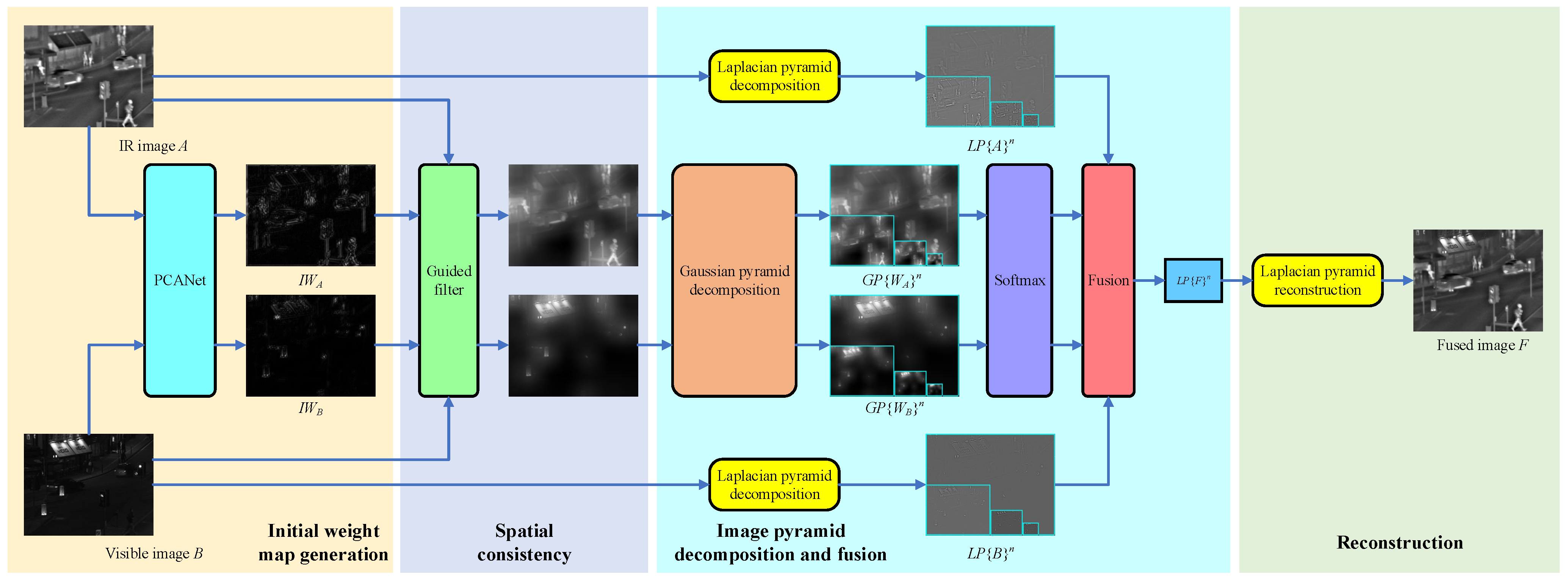
  • We propose a novel IR and visible image fusion method based on a PCANet and image pyramid, aiming to perform activity-level measurement and weight assignment through the lightweight deep learning model PCANet. The activity-level measurement obtained by the PCANet has a strong representation ability by focusing on IR target perception and visible-detail description.
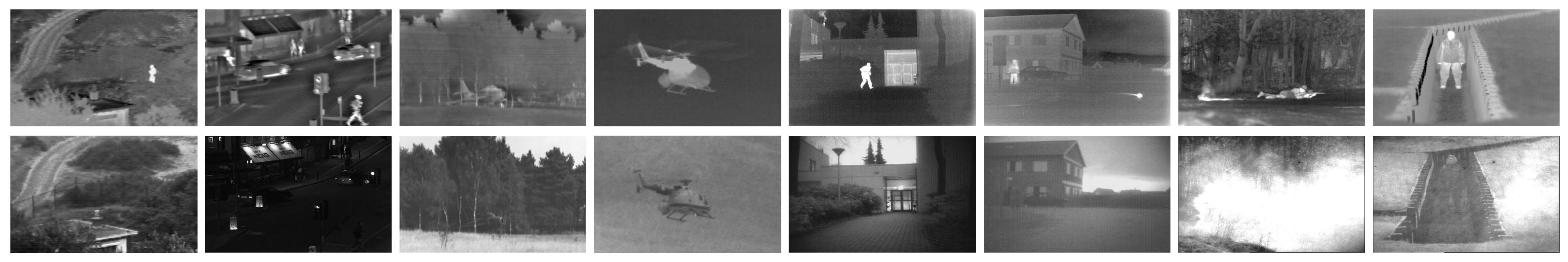
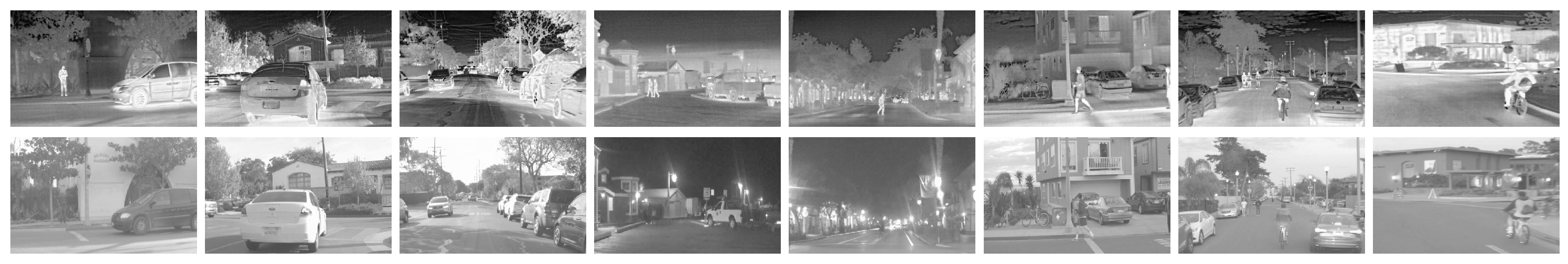
  • The effectiveness of the proposed algorithm was verified by 88 pairs of IR and visible images in total and 19 competitive methods, demonstrating that the proposed algorithm can achieve state-of-the-art performance in both visual quality and objective evaluation metrics.
The rest of the paper is arranged as follows: Section 2 briefly reviews PCANet, image pyramids, and guided filters. The proposed IR and visible image fusion method is depicted in Section 3. The experimental results and analyses are shown in Section 4. Finally, this article is concluded in Section 5.

2. Related Work

In this section, for a comprehensive review of some algorithms most relevant to this study, we focus on reviewing PCANet, the image pyramid, and the guided filter.

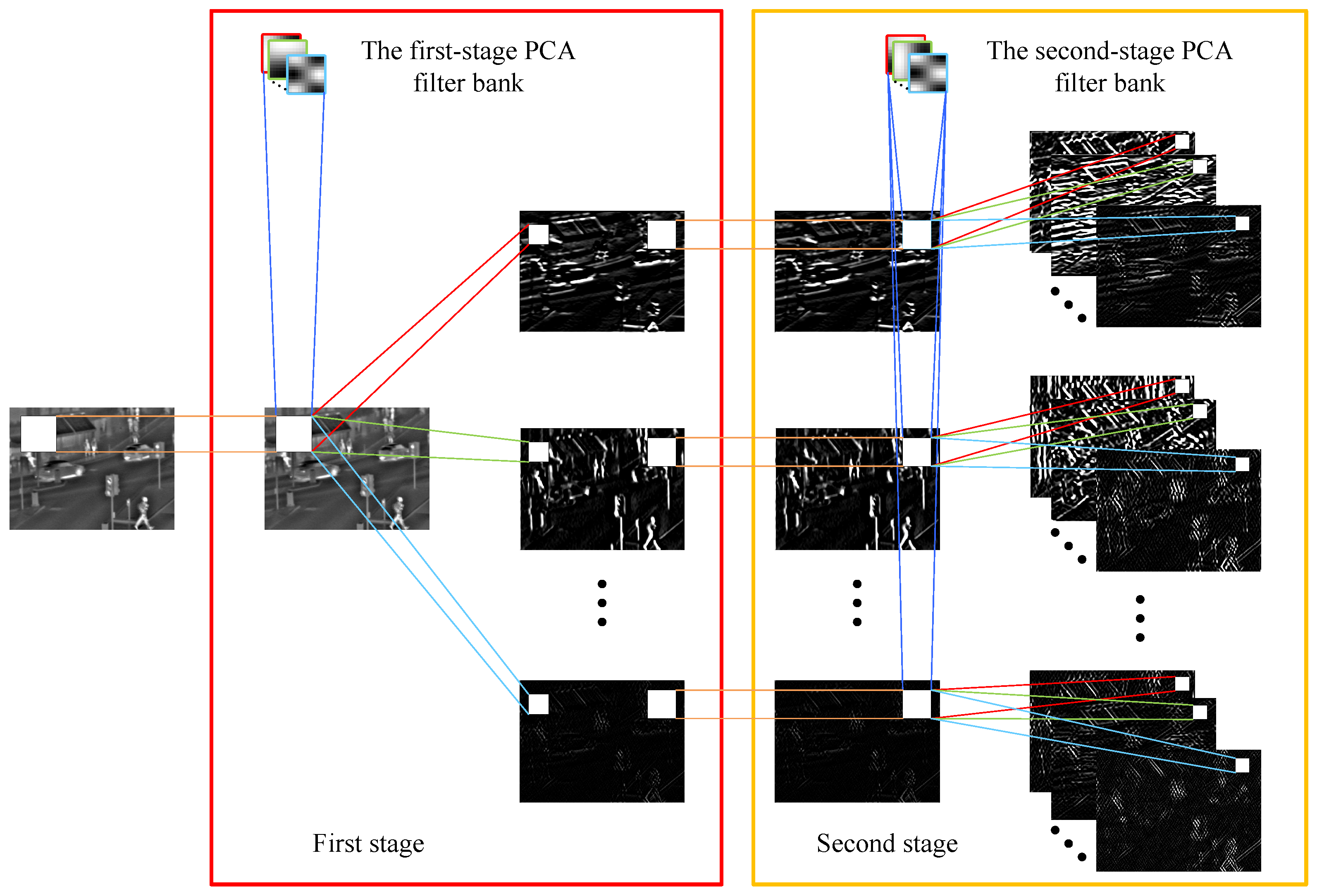
2.1. Principal Component Analysis Network (PCANet)

A principal component analysis network (PCANet) [22] is a lightweight, unsupervised deep learning neural network mainly used for extracting features in images, and it can also be considered as a simplified version of a CNN. In a PCANet, the critical task is the training of PCA filter, which will be specifically introduced in the next section. A PCANet consists of three components: cascaded two-stage PCA, binary hashing, and block histograms:
(1) Cascaded two-stage PCA: We assume that the filter bank W 1 in the first stage of the PCANet includes L 1 filters W 1 1 , W 2 1 , , W L 1 1 , and the filter bank W 2 in the second stage contains L 2 filters W 1 2 , W 2 2 , , W L 2 2 . Firstly, the input sample I is convolved with the l-th filter W l 1 of the first stage:
I l = I W l 1 , l = 1 , 2 , , L 1
where * represents the convolution operation. Then, I l is convolved with the r-th filter W r 2 of the second stage:
O q = I l W r 2 , l = 1 , 2 , , L 1 , r = 1 , 2 , , L 2 , q = 1 , 2 , , L 1 L 2
where O q represents the output of I and L 1 L 2 stands for the amount of output images.
(2) Binary hashing: Next, O q will be binarized, and then these binary matrices are converted to decimal matrices as:
T l = r = 1 L 2 2 r 1 H I l W r 2
where T l is the l-th decimal matrix for I, and H · is a Heaviside step function, whose value is one for positive entries and zero otherwise.
(3) Block histograms: In this part, each T l , l = 1 , , L 1 is split into B blocks, and we compute the histograms of the decimal values in each block and concatenate whole B histograms into one vector Bhist T l . Following this encoding process, the input image I is transformed into a set of block-wise histograms. We ultimately acquire the feature vectors as:
f = Bhist T 1 , , Bhist T L 1 T R 2 L 2 L 1 B
where f is the network output.
The advantages of a PCANet are twofold:
  • In the training stage, the PCANet obtains the convolution kernel through PCA auto-encoding does not need to iterate calculations of the convolution kernel like other deep learning methods.
  • As a lightweight network, PCANet has only a few hyperparameters to be trained.
These two advantages make PCANet more efficient. PCANet has a wide range of applications in various fields, such as image recognition [22], object detection [25,26], image fusion [27], and signal classification [28,29].

2.2. Image Pyramids

An image pyramid [3,23] is a collection of images that consists of multiple sub-images of different resolutions of an image. In an image pyramid, the top-layer image has the lowest resolution, and the bottom-layer images have the highest resolution. Image pyramids include Gaussian pyramid and Laplacian pyramid [3].
In the Gaussian pyramid, we use I to represent the original image, that is, the 0-th layer Gaussian pyramid G P 0 . We perform Gaussian filtering and interlaced subsampling on G P 0 to obtain the first layer of the Gaussian pyramid, G P 1 . Repeat the above operations to obtain G P 0 , G P 1 , , G P h , , G P N (where G P h is the h-th layer of the Gaussian pyramid).
The Gaussian pyramid can be expressed as:
G P 0 = I G P h = R E D U C E G P h 1
G P h i , j = m = 2 2 n = 2 2 G P h 1 2 i + m , 2 j + n s m , n
where i , j represents the coordinates in the image, i 0 , R h 1 , j 0 , C h 1 , and h 1 , N . N is the number of layers of Gaussian pyramid decomposition; R h and C h are the numbers of rows and columns of the h-th layer of the Gaussian pyramid, respectively; and s m , n is a 2D separable 5 × 5 window function. By combining Equations (5) and (6), we can get the Gaussian pyramid image sequence G P 0 , G P 1 , , G P N , and the upper layer is four times smaller than the lower layer.
On the other hand, we apply interpolation to enlarge the h-th layer Gaussian pyramid G P h to obtain the image G P h * :
G P h * = E X P A N D G P h
where the size of G P h * is the same as that of G P h 1 . G P h * can be denoted as:
G P h * i , j = 4 m = 2 2 n = 2 2 G P h i + m 2 , j + n 2 s m , n
where h 1 , N , i 0 , R h 1 , j 0 , C h 1 . When i + m i + m 2 2 and j + n j + n 2 2 are non-integers:
G P h i + m 2 , j + n 2 = 0 .
The expansion sequence G P 1 * , G P 2 * , , G P N * can be obtained by Equations (7)–(9).
The Laplacian pyramid can be expressed as:
L P h = G P h E X P A N D G P h + 1
L P h = G P h G h + 1 * , h 0 , N 1 L P N = G P N , h = N
where L P 0 , L P 1 , , L P N represent Laplacian pyramid images, and L P N is the top layer.
The inverse Laplacian pyramid transform (reconstruction) process can be obtained as follows:
G P N = L P N G P h = L P h + E X P A N D G P h + 1 , h 0 , N 1 I = G P 0
where I is the reconstructed image.

2.3. Guided Filter

A guided filter [30] is an edge filter based on a local linear model which does not need to perform convolution directly like most other filtering methods, and has simplicity, fast speed, and great edge-preservation. We define that filter output q is a linear transform of guidance image G I in a window ω k centered on pixel k:
q i = a k G I i + b k , i ω k
where a k and b k are the linear coefficients in ω k .
To determine a k and b k , we minimize the difference between the filter output q and the filter input p, i.e., the cost function:
E a k , b k = i ω k a k G I i + b k p i 2 + ϵ a k 2
where ϵ is a regularization parameter that serves to prevent a k from being too large. With the above equation, we can enable the local linear model maximally similar to the input image p in ω k .
a k and b k can be obtained by the following:
a k = 1 ω i ω k G I i p i μ k p ¯ k σ k 2 + ϵ
b k = p ¯ k a k μ k .
In the above equations, μ k and σ k 2 are the mean and variance of G I in ω k , ω is the number of pixels in ω k , and p ¯ k = 1 ω i ω k p i is the mean of p in ω k .
We employ this linear model to all the local windows of the input image, but these windows are overlapped, and their centers are located in ω k . Thus, the filter output is averaged over all possible q i values by:
q i = a ¯ i G I i + b ¯ i
where a ¯ i = 1 ω k ω i a k and b ¯ i = 1 ω k ω i b k are the mean coefficients acquired from whole the overlapped windows, including pixel i.
Guided filter is performed by combining Equations (13)–(17), which can be simply denoted by:
q = G u i d e d F i l t e r G I , p
where p indicates the input image, G I denotes the guidance image, and q represents the filter output.

3. The Proposed Method

We propose a novel IR and visible fusion method based on PCANet and an image pyramid. The activity-level measurement and weight assignment are two key parts of image fusion. We used PCANet to perform activity-level measurement and weight assignment because PCANet has stronger representation ability by focusing on IR target perception and visible detail description. Due to the human visual system processing information in a multi-resolution way [24], we apply an image pyramid to decompose and merge the images at multiple scales in order to make the fused image details appear more suitable for human visual perception.

3.1. Overview

The proposed algorithm is exhibited in Figure 1. Our method consists of four steps: PCANet initial weight map generation, spatial consistency, image-pyramid decomposition and fusion, and reconstruction. In the first step, we feed the two source images into PCANet and get the initial weight maps. In the second step, we take advantage of the spatial consistency to improve the quality of initial weight maps. The third step is image-pyramid decomposition and fusion. On the one hand, the source images are multi-scale transformed through the Laplacian pyramids. On the other hand, the initial weight maps are decomposed into multiple scales through Gaussian pyramids, and the softmax operation is performed on each scale to obtain the weight maps of each layer. Then, the fused image of each scale is obtained through a weighted-average strategy. In the last step, the final fusion image is obtained by reconstructing the Laplacian pyramid.

3.2. PCANet Design

In our study, IR and visible image fusion is treated as a two-class classification problem. For each pixel from the same position of the source images, a scalar from 0 to 1 is output through PCANet to represent the probability of coming from different source images in the fused image. Standard PCANet contains cascaded two-stage PCA, binary hashing, and block histograms, where the role of the latter two components is to extract sparse features of images. If the network includes binary hashing and block histograms, the output sparse features have only two values of zero and one, and the size of the features are inconsistent with the source images. In our fusion task, in order to obtain more accurate probability values of the same position pixel from two source images and perform the fusion task faster, we only use cascaded two-stage PCA. The network design of PCANet is shown in Figure 2. In PCANet, the most important component is the PCA filter. In the next section, we describe the training process of the PCA filter in detail. In the PCANet framework, firstly, the input image is convolved with the first-stage PCA filter bank to obtain a series of feature maps. Then, these feature maps are convolved with the second-stage PCA filter bank to obtain more feature maps. These feature maps represent the details of the input image on different objects. Particularly, the second-stage filters can extract more advanced features. Two-stage PCA is usually sufficient to obtain a great effect, and a deeper architecture does not necessarily lead to further improvements [22], so we selected cascaded two-stage PCA for our experiments.

3.3. Training

The training of PCANet is essentially computing the PCA filter. PCA can be viewed as the simplest class of an auto-encoder, which minimizes reconstruction error [22]. We selected N images in the MS-COCO [31] database for training. In our experiments, we set N to 40,000. Considering that the size of each image in the MS-COCO database is different, each training image was converted into a 256 × 256 grayscale image. The training process of PCANet consisted of calculating two-stage PCA filter banks, and we assume that each filter size was k 1 × k 2 in both stages. In the following, we describe the training process of each stage in detail.
  • The First Stage
In order to facilitate the convolution operation, each training image is preprocessed. Preprocessing contains two steps: (1) Each sliding k 1 × k 2 patch in the i-th training image I i was converted into a column of X i , where X i = x i , 1 , x i , 2 , , x i , m ˜ n ˜ R k 1 k 2 × m ˜ n ˜ , i = 1 , 2 , N , m ˜ = 256 k 1 + 1 , n ˜ = 256 k 2 + 1 . (2) The patch mean is subtracted from each column in X i to obtain X ¯ i = x ¯ i , 1 , x ¯ i , 2 , , x ¯ i , m ˜ n ˜ R k 1 k 2 × m ˜ n ˜ .
After the above preprocessing, we perform the same operation on N training images to obtain X = X ¯ 1 , X ¯ 2 , , X ¯ N R k 1 k 2 × N m ˜ n ˜ . Then, we compute the covariance matrix C 1 of X:
C 1 = X X T N m ˜ n ˜ .
Next, by calculating the eigenvalue Λ 1 and eigenvector Q 1 of the covariance matrix C 1 , we can obtain:
C 1 = Q 1 Λ 1 Q 1 T
where Λ 1 is a diagonal matrix with k 1 k 2 eigenvalues on the diagonal. Each column in Q 1 indicates an eigenvector corresponding to the eigenvalue in Λ 1 , that is, the PCA filter. Particularly, the larger the eigenvalue, the more important the corresponding principal component. Therefore, we select the eigenvectors corresponding to the top L 1 largest eigenvalues as the PCA filters. Accordingly, the l-th PCA filter can be expressed as W l 1 , l = 1 , 2 , , L 1 . Clearly, the PCA filter bank of the first stage is denoted as:
W 1 = W 1 1 , W 2 1 , , W L 1 1 .
Actually, the role of the PCA filter bank is to capture the main changes in the input image [22]. Next, we zero-pad the height and width boundaries of the i-th image I i with size k 1 1 and size k 2 1 , respectively, so that the convolution outputs have the same size as the source image. Then, I i is preprocessed to obtain I ¯ i . The I ¯ i is convolved with the l-th PCA filter in the first stage to obtain:
T i l = I ¯ i W l 1 , i = 1 , 2 , , N , l = 1 , 2 , , L 1
where * represents the convolution operation and T i l indicates an input sample of the second stage.
  • The Second Stage
Firstly, almost the same as the first stage, the input image T i l is preprocessed to obtain Y ¯ i l = y ¯ i , l , 1 , y ¯ i , l , 2 , , y ¯ i , l , m ˜ n ˜ R k 1 k 2 × m ˜ n ˜ , and then the i-th input image is represented as Y i = Y ¯ i 1 , Y ¯ i 2 , , Y ¯ i L 1 R k 1 k 2 × L 1 m ˜ n ˜ . Performing the same for all N input images, we obtain Y = Y 1 , Y 2 , , Y N R k 1 k 2 × N L 1 m ˜ n ˜ . Next, similar to the first stage, we compute the covariance matrix C 2 of Y:
C 2 = Y Y T N L 1 m ˜ n ˜
C 2 = Q 2 Λ 2 Q 2 T
where Λ 2 denotes the eigenvalues of the second stage, and Q 2 represents the eigenvectors of the second stage. We select the eigenvectors corresponding to the top L 2 largest eigenvalues as the filter bank of the second stage. Therefore, the r-th PCA filter in the second stage can be denoted as W r 2 , r = 1 , 2 , , L 2 . The PCA filter bank of the second stage is indicated as:
W 2 = W 1 2 , W 2 2 , , W L 2 2 .
Up till this point, the two-stage filter banks W 1 and W 2 of PCANet have been obtained. The difference between the filters of the two stages is that the second-stage filters can extract higher-level features than the first-stage.

3.4. Detailed Fusion Scheme

3.4.1. PCANet Initial Weight Map Generation

Let the input image A indicate an IR image and B represent a visible image, and they are pre-registered images with the same size. Assume that each PCA filter size is k 1 × k 2 in both stages. Firstly, we zero-pad the height and width boundaries of A and B with size k 1 1 and size k 2 1 , respectively, so that the convolution outputs have the same size as the source images. Next, the input image S, S A , B , takes advantage of the preprocessing to obtain S ¯ R k 1 k 2 × m ˜ n ˜ . The S ¯ is convolved with the l-th PCA filter in the first stage:
T S l = S ¯ W l 1 , l = 1 , 2 , , L 1 .
Through the first-stage filter bank W 1 , the first-stage PCANet outputs a total of L 1 feature maps T S 1 , T S 2 , , T S L 1 .
The second stage is similar to the first stage. Firstly, zero-padding is performed in each T S l , and then preprocessing is taken to obtain U ¯ S l R k 1 k 2 × m ˜ n ˜ . Next, U ¯ S l is convolved with the r-th PCA filter in the second stage:
O S q = U ¯ S l W r 2 , l = 1 , 2 , , L 1 , r = 1 , 2 , , L 2 , q = 1 , 2 , , L 1 L 2 .
The second-stage PCANet outputs a total of L 1 L 2 feature maps O S 1 , O S 2 , , O S L 1 L 2 .
Next, we define the initial weight maps for IR image A and visible image B as I W A and I W B :
I W A x , y = O A 1 x , y + O A 2 x , y + + O A L 1 L 2 x , y
I W B x , y = O B 1 x , y + O B 2 x , y + + O B L 1 L 2 x , y
where x and y represent the coordinates of the pixels in the image. Particularly, I W A and I W B are the same size as the source images.

3.4.2. Spatial Consistency

Spatial consistency means that two adjacent pixels with similar brightness or color will have a greater probability of having similar weights [32]. The initial weight maps are in general noisy, which may create artifacts on the fused image. To improve the performance of fusion, the initial weight maps need to be further processed. Specifically, we utilize a guided filter [30] to improve the quality of the initial weight maps. The guided filter is a very effective edge-preserving filter which can transform the structural information of the guided image into the filtering result of the input image [30]. We adopt the source image S as the guidance image to guide the absolute value of the initial weight map for filtering:
I W A = G u i d e d F i l t e r A , I W A
I W B = G u i d e d F i l t e r B , I W B
where A and B represent guidance images. In guided filter, we experimentally set the local window radius to 50 and the regularization parameter to 0.1.

3.4.3. Image-Pyramid Decomposition and Fusion

We perform n-layer Gaussian pyramid decomposition [3,23] on I W A and I W B to obtain G P W A n and G P W B n according to Equations (5) and (6). Each pyramid decomposition layer is set to the value log 2 min H i g , W i d , where H i g × W i d is the spatial size of source images and · denotes the flooring operation. Then, G P W A n and G P W B n are fed into a 2-way softmax layer, which produces probability values for two classes, denoting the outcome of each weight assignment:
F W A ( x , y ) n = e G P W A ( x , y ) n e G P W A ( x , y ) n + e G P W B ( x , y ) n
F W B ( x , y ) n = e G P W B ( x , y ) n e G P W A ( x , y ) n + e G P W B ( x , y ) n .
The values of F W A n and F W B n are between zero and one, indicating the probabilities that A and B take values at the same position pixel point. After the above operations, the network can autonomously learn the features in the image and calculate the weight of each pixel, avoiding the complexity and subjectivity of manually designing the fusion rules.
In addition, we conduct n-layer Laplacian pyramid decomposition [3,23] on A and B to obtain L P A n and L P B n according to Equations (10) and (11). The number of the Laplacian pyramid’s decomposition layers is the same as that of the Gaussian pyramid. It is noteworthy that F W A n and F W B n are the same sizes as L P A n and L P B n . Then, the fused image L F n on each layer is obtained by the weighted-average rule:
L F ( x , y ) n = F W A ( x , y ) n × L P A ( x , y ) n + F W B ( x , y ) n × L P B ( x , y ) n .

3.4.4. Reconstruction

Finally, we reconstruct the Laplacian pyramid L F n to obtain the fused image F according to Equation (12). The main steps of the proposed IR and visible image fusion method are summarized in Algorithm 1.
Algorithm 1 The proposed IR and visible image fusion algorithm.
Training phase
1. Initialize PCANet;
2. Calculate the first-stage PCA filter bank W 1 via Equations (19)–(22);
3. Calculate the second-stage PCA filter bank W 2 via Equations (23)–(25).
Testing (fusion) phase
Part 1: PCANet initial weight map generation
1.  Feed IR image A and visible image B into PCANet to obtain the initial weight maps according to Equations (26)–(29);
Part 2: Spatial consistency
2.  Perform guided filtering on the absolute values of I W A and I W B according to Equations (30) and (31);
Part 3: image-pyramid decomposition and fusion
3.  Perform n-layer Gaussian pyramid decomposition on I W A and I W B to generate the results G P W A n and G P W B n according to Equations (5) and (6);
4.  Perform softmax operation at each layer to obtain F W A n and F W B n according to Equations (32) and (33);
5.  Perform n-layer Laplacian pyramid decomposition on A and B to obtain L P A n and L P B n according to Equations (10) and (11);
6.  Apply the weighted-average rule on each layer to generate the result L F n according to Equation (34);
Part 4: Reconstruction
7.  Reconstruct the Laplacian pyramid to obtain the fused image F according to Equation (12).

4. Experiments and Discussions

In this section, the two experimental datasets and thirteen objective quality metrics are introduced. Secondly, the effects of different sizes and various number of filters in our method are discussed. Thirdly, we verify the effectiveness of our algorithm through two ablation studies. Fourthly, the proposed algorithm is evaluated by using visual quality and objective evaluation metrics. We selected nineteen state-of-the-art fusion methods to compare with our algorithm. Finally, we show the computational efficiency of different algorithms. All our experiments were performed on Intel (R) Core (TM) i7-11700, 64 GB RAM, and MATLAB R2019a.

4.1. Datasets

In order to comprehensively verify the effectiveness of our algorithm, we selected two datasets of different scenes for experiments, namely, the TNO dataset [33] and the RoadScene [34] dataset. The TNO dataset consists of several hundred pairs of pre-registered IR and visible images, mainly including military-related scenes, such as camps, helicopters, fighter jets, and soldiers. We chose 44 pairs of images in TNO dataset as test images. Figure 3 exhibits eight pairs of testing images of the TNO dataset, where the top row represents the IR images and the bottom row denotes the visible images.
Differently from the TNO dataset, the RoadScene dataset has 221 pairs of road-related IR and visible pre-registered images, mainly including scenes of rural roads, urban roads, and night roads. We selected 44 pairs of images in the RoadScene dataset as test images. Figure 4 exhibits eight pairs of testing images of the RoadScene dataset, where the top row indicates the IR images and the bottom row denotes the visible images.

4.2. Objective Image Fusion Quality Metrics

In order to verify the fusion effect of our algorithm, we selected 13 objective evaluation metrics to conduct experiments. In what follows, we precisely describe various evaluation metrics:
  • Yang’s metric Q Y [35]: Q Y is a fusion metric based on structural information, which aims to calculate the degree to which structural information is transferred from the source images into the fused image;
  • Gradient-based metric Q G [36]: Q G provides a fusion metric of image gradient, which reflects the degree of edge information of the source images preserved in the fusion image;
  • Structural similarity index measure S S I M [37]: S S I M is a fusion index based on structural similarity, which mainly calculates the structural similarity between the fusion result and the source images;
  • F M I w , F M I d c t and F M I p i x e l [38] calculate wavelet features, discrete cosine, and feature mutual information (FMI), respectively;
  • Modified fusion artifacts measure N a b f [39]: N a b f provides a fusion index that introduces noise or artifacts in the fused image, reflecting the proportion of noise or artifacts generated in the fused image;
  • Piella’s three metrics Q S , Q W , Q E [40]: Piella’s three measures are on the basis of the structural similarity between source images and the fused image;
  • Phase-congruency-based metric Q P [41]: Q P calculates the degree to which salient features in the source images are transferred to the fused image, and it is based on the absolute measure of image features;
  • Chen–Varshney metric Q C V [42]: The metric Q C V is based on the human vision system and can fit the results of human visual inspection well;
  • Chen–Blum metric Q C B [43]: Q C B is a fusion metric based on human visual perception quality.
In the above metrics, except N a b f and Q C V , the larger the values, the better the fusion performance. On the contrary, the smaller the values of N a b f and Q C V , the better the fusion effect. Among all the metrics, S S I M , N a b f , and Q C B are the most important.

4.3. Analysis of Free Parameters

PCANet is a lightweight network with only three free parameters: the number of first-stage filters L 1 , the number of second-stage filters L 2 , and the size of the filter. We set the filter sizes of the two stages to be the same. We used the 44 pairs of images in TNO dataset to perform parameter setting experiments. The fusion performance is calculated by the average values of 13 fusion metrics, and the best values are indicated in red.

4.3.1. The Effect of the Number of Filters

We discuss the effect of the number of filters on fusion performance. As shown in Table 1, we fixed the PCA filter size to 3 × 3 , and then the number of first-stage filters L 1 and the number of second-stage filters L 2 were set to vary from 3 to 8. In PCANet, the number of L 1 and L 2 affects the feature extraction of input samples. A higher number of filters means that the model extracts more features. Table 1 shows the influences of different numbers of L 1 and L 2 on the fusion performance. When L 1 = L 2 = 8, the model obtains 10 best values. If the values of L 1 and L 2 are greater than eight, the model will take more time, and the value of S S I M may be lower. We should keep the model as simple as possible, so we set L 1 = L 2 = 8.

4.3.2. The Influence of Filter Size

In this experiment, we discuss the impact of filter size on fusion performance. In Table 2, we fixed L 1 = L 2 = 8, and then the sizes of PCA filters were set to 3 × 3 , 5 × 5 , 7 × 7 , 9 × 9 , and 11 × 11 , respectively. In PCANet, different filter sizes affect receptive field and feature extraction. A larger filter size means that the model extracts more features. Table 2 exhibits the influence of different filter size on the fusion performance. One can see that the fusion performance is the best when the size of the PCA filter is 11 × 11 .
Therefore, we set L 1 = L 2 = 8, and the PCA filter size was 11 × 11 .

4.4. Ablation Study

In this part, we conducted two ablation studies to verify the effectiveness of the image pyramid and guided filter.

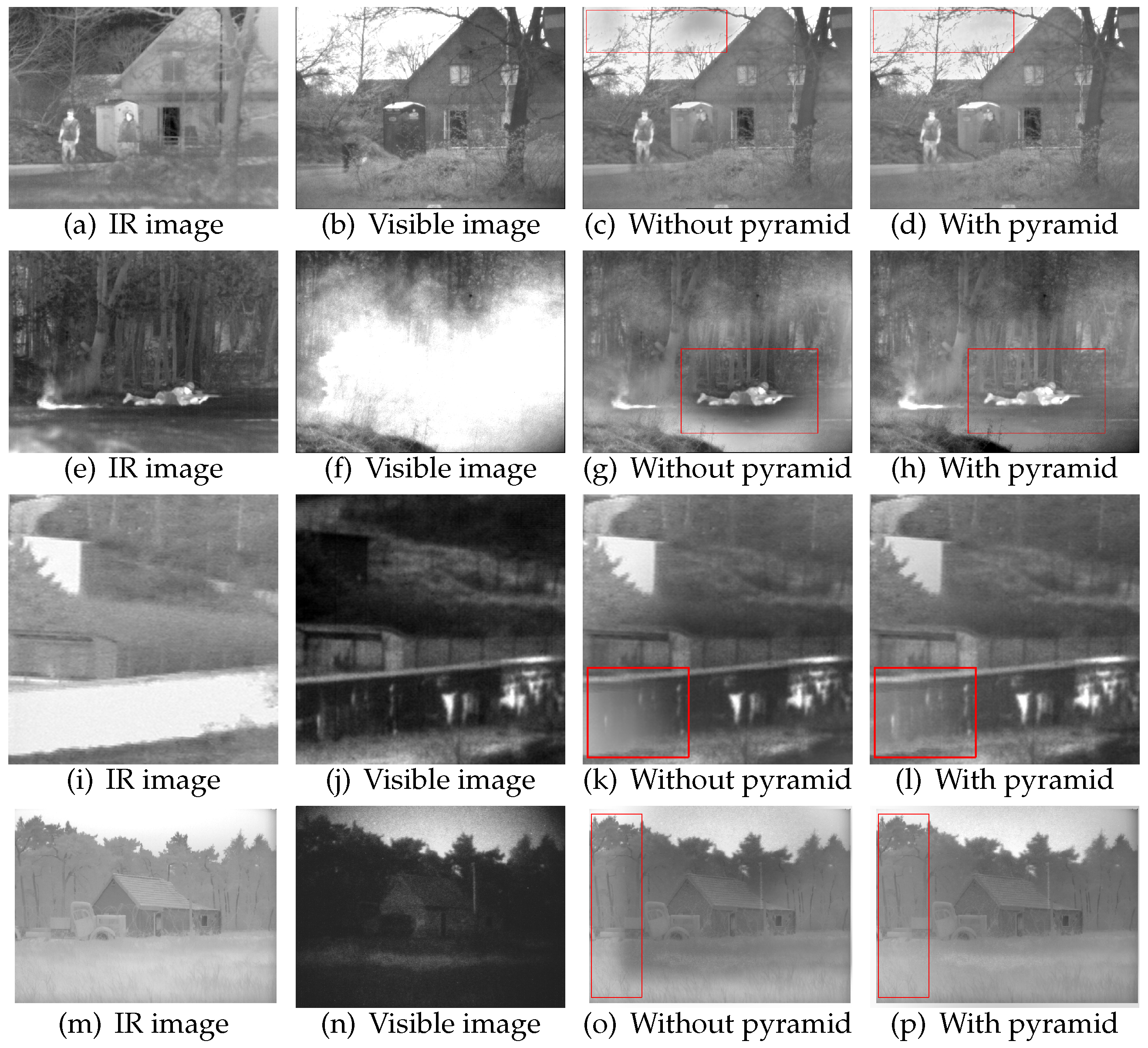
4.4.1. The Ablation Study of the Image Pyramid

Figure 5 shows the results of image pyramid ablation experiment. We compared the model with and without image pyramids regarding the fusion results. The first column represents the IR image, the second column denotes the visible image, the third column indicates the model without the image pyramid, and the fourth column represents the model with the image pyramid. Except the image pyramid, other parameters were the same. For the four examples, the fusion results for the model with the image pyramid are better than the fusion results for the model without the image pyramid. The fusion results for without the pyramid introduce some artifacts and noises, and the model with the pyramid almost eliminated these artifacts and the noise through multi-scale decomposition (see the red boxes in Figure 5).
We used the 44 pairs of images in the TNO dataset to verify the effect of the model with and without image pyramids. Table 3 shows the average value of each evaluation index and the fusion time for 44 pairs of images. The best values are indicated in red. The running times of the two models were almost the same, and the model with image pyramid obtained eight optimal values. Combined with visual quality and objective evaluation metrics, it is proved that the algorithm with the image pyramid is better.

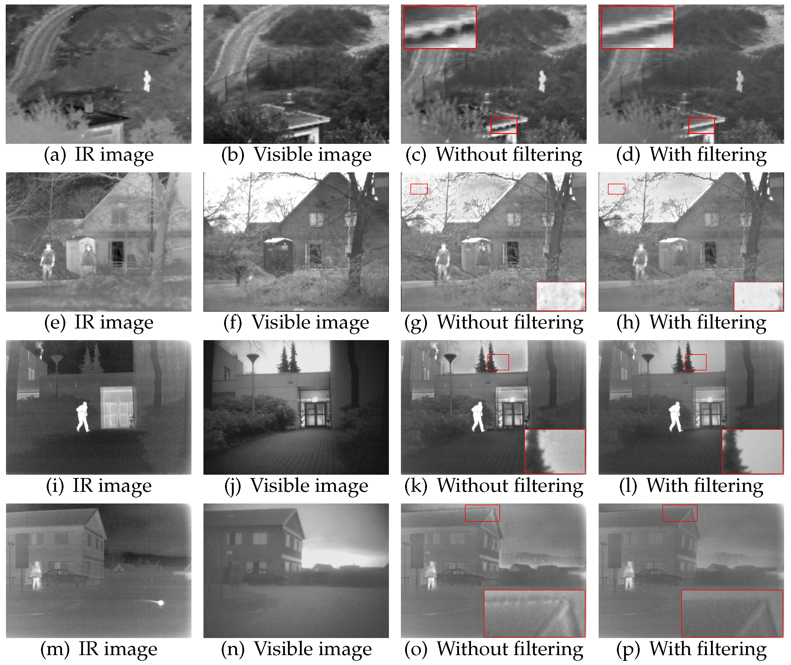
4.4.2. The Ablation Study of the Guided Filter

Figure 6 shows the results of the guided-filter ablation experiment. We compare the model with and without guided filtering. The first column has IR images, the second column has visible images, the third column has images produced without guided filtering, and the fourth column has images produced with guided filtering. All other parameter settings were the same. There are some obvious artifacts and noise in the red boxes in the third column of Figure 6. After guided filtering, these artifacts and the noise were eliminated. It can be seen in the figure that the fusion effect with guided filtering is better.

4.5. Experimental Results and Discussion

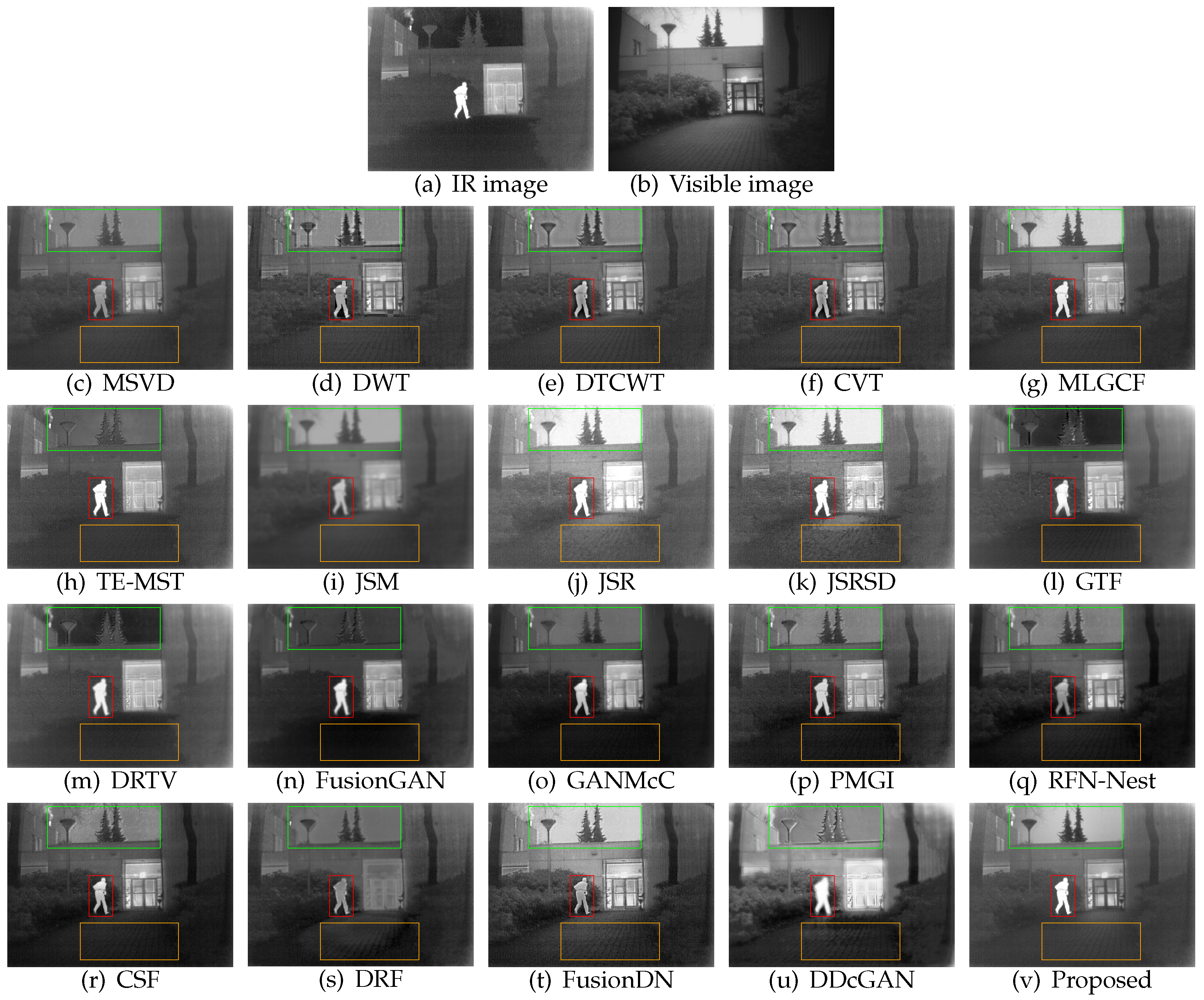
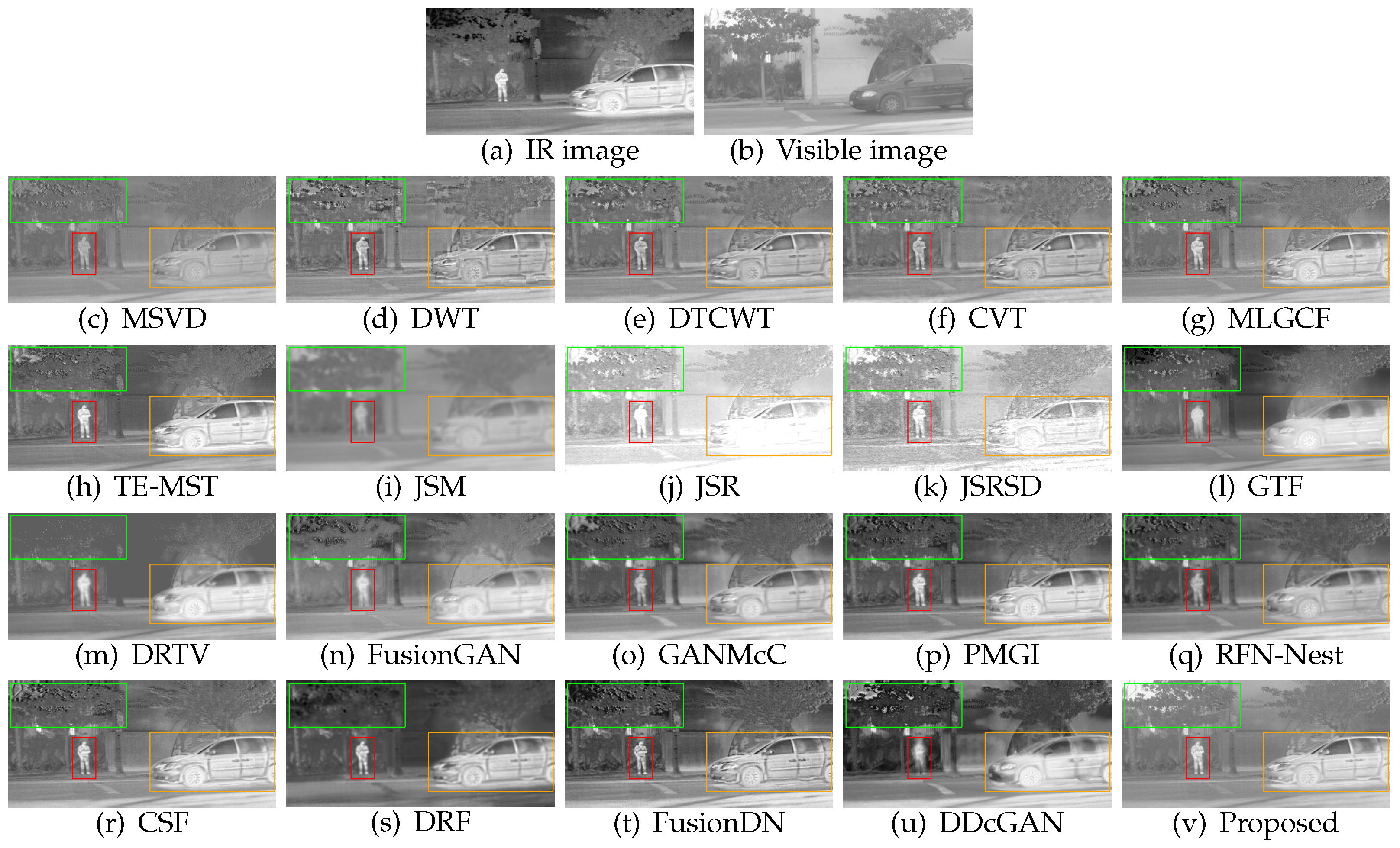
4.5.1. Comparison with State-of-the-Art Competitive Algorithms on the TNO Dataset

We used the TNO dataset to verify the performance of our algorithm. The competitive algorithms numbered 19: MST methods (MSVD [4], DWT [5], DTCWT [6], CVT [7], MLGCF [44], and TE-MST [8]), SR methods (JSM [9], JSR [10], and JSRSD [11]), deep learning methods (FusionGAN [19], GANMcC [21], PMGI [45], RFN-Nest [46], CSF [13], DRF [47], FusionDN [34], and DDcGAN [20]), and other methods (GTF [48] and DRTV [49]). In particular, the comparative algorithms based on deep learning have been proposed in the last three years. The corresponding parameter settings in the comparison algorithms were set to the default values given by their authors.
In our approach, we set the filter size to 11 × 11 for both stages, and the number of filters to eight for both stages. The number of image-pyramid decomposition layers was n, n = lo g 2 min H i g , W i d , where H i g × W i d represents the size of the source images and · denotes the flooring operation. We set the radius of the guided filter to 50 and the regularization parameter to 0.1. The fusion performance of the proposed method was evaluated by comparing the visual quality and objective evaluation metrics.
Figure 7 and Figure 8 show two representative examples. For better comparison, some regions in the fused images are marked with rectangular boxes. Figure 7 shows the fusion results of “Queen Road” source images. The described nighttime scene includes rich content, containing pedestrians, cars, street lights, and shops. IR images exhibit thermal radiation information of pedestrians, vehicles, and street lights, while visible images provide clearer details, especially the details of the plate of storefront. The ideal fusion result of this example is to preserve the thermal radiation information in the IR image while extracting the details in the visible image. Pedestrians in the MSVD, DTCWT, and CVT methods suffer from low brightness and contrast (see red and orange boxes in Figure 7c,e,f). The DWT-based method introduces undesired small rectangular blocks (see three boxes in Figure 7d). Although the MLGCF algorithm can extract the thermal objects well, the whole image is too dark. The TE-MST technique has high fusion quality, but it introduces too much of the infrared spectrum to the plate of storefront, resulting in an unnatural visual experience (see the green box in Figure 7h). The plate of storefront in the JSM fusion result is clearly blurred (see the green box in Figure 7i). Although JSR and JSRSD schemes achieve a great fusion effect, their backgrounds lack some details. Both GTF and DRTV methods suffer from low fusion performance, especially the lack of details on the plate of storefront (see green boxes in Figure 7l,m). Among the deep-learning-based algorithms, the FusionGAN, GANMcC, PMGI, and RFN-Nest methods cannot extract the details of the plate of storefront well due to introducing too much of the infrared spectrum (see the green boxes in Figure 7n,o,p,q). The CSF technique cannot extract thermal radiation information well (see the red and orange boxes in Figure 7r). The DRF, FusionDN, and DDcGAN methods appear overexposed and introduce some undesired noise (see Figure 7s,t,u). Our algorithm can well extract thermal radiation objects in the IR image and details in the visible image with a more natural visual experience (see Figure 7v). Our algorithm has the stronger representation ability by focusing on IR target perception and visible detail description compared with other methods.
Figure 8 shows the fusion results of the “Kaptein” source images, which exhibit a person standing at a door. On the one hand, IR images mainly capture the thermal radiation information of person. On the other hand, the visible images clearly show the details of buildings, trees in the distance, and grass. The person after MSVD, DWT, DTCWT, and CVT methods suffers from low brightness and contrast. In particular, the DWT, DTCWT, and CVT algorithms produce some artifacts around the people. The MLGCF and TE-MST methods cannot well extract the details of the ground textures (see the orange boxes in Figure 8g,h). The JSM fusion result is blurry, and JSR and JSRSD schemes introduced some noise. The GTF and DRTV methods introduce artifacts around distant trees. Regarding the deep learning algorithms, the man after application of the FusionGAN and DDcGAN methods is blurry, and the person after the RFN-Nest and DRF methods has low brightness. These fusion results constitute an unnatural visual experience. In addition, the GANMcC, PMGI, and CSF methods cannot well capture the details of the sky and ground (see the orange and green boxes in Figure 8o,p,r). The FusionDN technique achieves high fusion performance. Compared to other methods, our method obtains better perceptual quality for the sky (see green box in Figure 8v), higher brightness of the thermal radiation objects (see red box in Figure 8v), and clearer ground textures (see orange box in Figure 8v).
Table 4 shows the averages of 13 objective evaluation metrics for the TNO dataset, and the best values are indicated in red. As can be seen in Table 4, except F M I d c t and Q E , our algorithm obtained the best results for all metrics, indicating that our algorithm has excellent fusion performance.

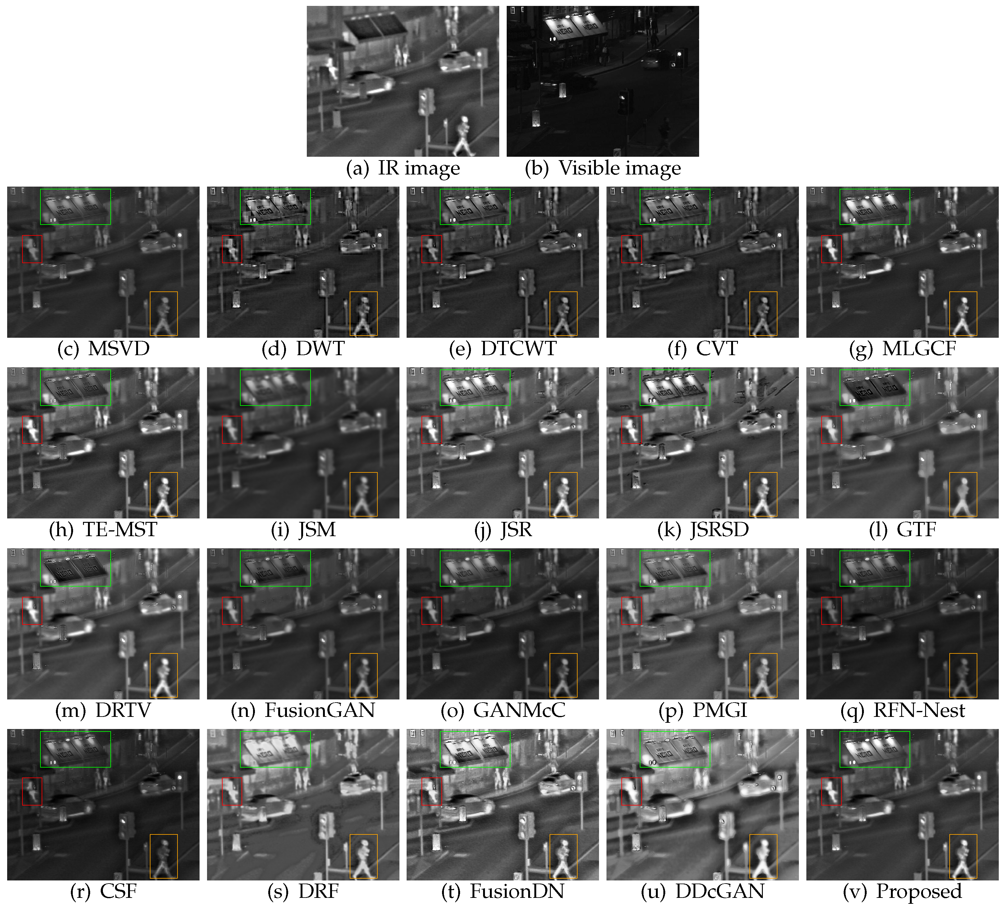
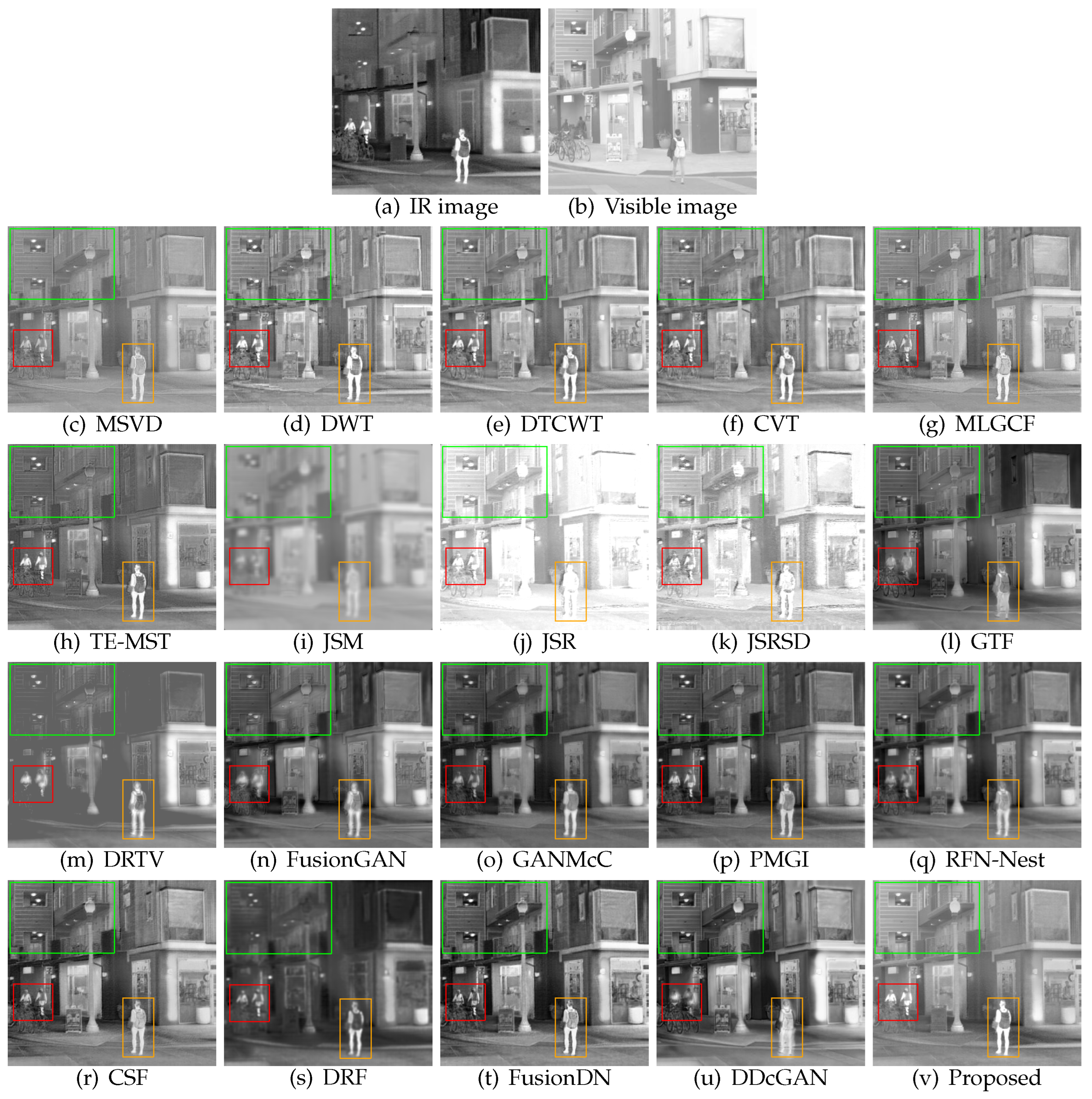
4.5.2. Further Comparison on the RoadScene Dataset

In order to verify the fusion performance in different scenes, we employed the RoadScene dataset for experiments. Figure 9 and Figure 10 show two representative examples. Figure 9 exhibits the fusion results of “FLIR04602” source images. The scene shows a pedestrian standing on the side of the road and a car parked on the road during the daytime. The IR images mainly capture the thermal radiation information of pedestrian and car, and visible images show the details of buildings and trees. The pedestrian and car in the MSVD method lost brightness and contrast. The DWT method introduces undesired “small rectangles” (see car and buildings in Figure 9d). The trees in the DTCWT, CVT, MLGCF, and TE-MST methods introduce too many “small black spots” from the infrared spectrum, resulting in unnatural visual experience (see green boxes in Figure 9e–h). The fusion result of JSM method is noticeably blurry. The JSR and JSRSD results appear overexposed. In particular, the JSRSD method introduces a certain amount of noise. The pedestrian and car became blurry by the GTF and DRTV methods. Regarding deep-learning-based methods, the fusion results of FusionGAN, DDcGAN, and DRF appear blurry. Specifically, the pedestrian and car through FusionGAN and DDcGAN methods were blurred, and trees and buildings through the DRF method were blurred. Since this example is a daytime scene, most of the visible image details are required. Although GANMcC, PMGI, RFN-Nest, CSF, and FusionDN methods achieved a good fusion effect, too many “small black dots” from IR images were introduced into the trees, resulting in an unnatural visual experience (see green boxes in Figure 9o–r,t). Compared with other algorithms, our algorithm can extract the pedestrian and car in the IR images well, and the results look more natural.
Figure 10 shows the fusion results of “FLIR08835” source images. The described scene contains rich content, including pedestrians, a street, and buildings. On the one hand, the IR image mainly extracts the thermal radiation information of the pedestrians to better display the locations of pedestrians. On the other hand, visible image provides clearer background details. The MSVD algorithm cannot extract thermal radiation information well. The DWT, DTCWT, CVT, TE-MST, and MLGCF fusion results all introduce some noise. The JSM fusion result is blurry, and JSR and JSRSD methods appear overexposed. The GTF method achieved great fusion performance, and the background areas in the DRTV algorithm’s images are obviously blurry (see the green box in Figure 10m). The pedestrians in the FusionGAN, DRF, RFN-Nest and DDcGAN algorithms’ images are blurry (see red and orange boxes in Figure 10n,s,q,u). The CSF method introduced some noise into the background. The GANMcC, PMGI, and FusionDN schemes achieved high fusion performance. Based on the above observations, it is clear that our algorithm captures the thermal radiation information of pedestrians well and has a great fusion effect. It can be at least stated that our method achieves competitive performance with the GANMcC, PMGI, and FusionDN methods.
Table 5 shows the averages of 13 objective evaluation metrics for the RoadScene dataset and the best values are indicated in red. It can be seen in Table 5 that, except for Q W , Q E , Q C V , and Q C B , the proposed fusion method achieved the best results for all other metrics.
Overall, it was found that the 19 competitive algorithms all suffer from some defects. Considering the above comparisons in relation to visual quality and objective evaluation metrics together, our algorithm can generally outperform other methods, leading to state-of-the-art fusion performance.

4.6. Computational Efficiency

To compare the computational efficiency, we ran all deep learning algorithms on the TNO dataset 10 times and took the average running time. It is worth noting that our experimental hardware environment was an Intel (R) Core (TM) i7-11700 with 64 GB RAM, but the experimental environments for various algorithms were different. The FusionGAN, GANMcC, PMGI, CSF, DRF, FusionDN, and DDcGAN methods used TensorFlow (CPU version). The RFN-Nest method used Pytorch (CPU version). Our algorithm was implemented in Matlab. All parameters in the comparison algorithms were the default values given by their authors. Table 6 shows the average time of 10 operations, and the optimal value is shown in red font. The running time of our algorithm achieved fourth place, namely, 255.6642 s, behind PMGI, FusionGAN, and RFN-Nest methods. Although the running time of our algorithm obtained fourth place, our fusion effect is state of the art.

5. Conclusions

In this paper, we propose a fusion method for IR and visible images based on PCANet and the image pyramid method. We use PCANet to obtain the activity-level measurement and weight assignment and apply an image pyramid to decompose and merge the images in multiple scales. The activity-level measurement obtained by PCANet has the stronger representation ability in focusing on IR target perception and visible detail description. We performed two ablation studies to verify the effectiveness of the image pyramid and the guided filter. Compared with nineteen representative methods, the experimental results demonstrated that the proposed method can achieve the state-of-the-art performance in both visual quality and objective evaluation metrics. However, we only used the results of the second stage of PCANet as image features, ignoring the useful information of the first stage. In the future research, we will explore combining features of multiple stages for fusion tasks.

Author Contributions

Conceptualization, S.L.; methodology, S.L.; software, S.L.; validation, S.L., G.W., Y.Z. and C.L.; formal analysis, S.L.; investigation, S.L.; data curation, S.L.; writing—original draft preparation, S.L.; writing—review and editing, S.L., G.W. and Y.Z.; project administration, G.W. and Y.Z.; funding acquisition, G.W. and Y.Z. All authors have read and agreed to the published version of the manuscript.

Funding

This work was financially supported by the National Natural Science Foundation of China (62175054, 61865005, and 61762033), the Natural Science Foundation of Hainan Province (620RC554 and 617079), the Major Science and Technology Project of Haikou City (2021-002), the Open Project Program of Wuhan National Laboratory for Optoelectronics (2020WNLOKF001), the National Key Technology Support Program (2015BAH55F04 and 2015BAH55F01), the Major Science and Technology Project of Hainan Province (ZDKJ2016015), and the Scientific Research Staring Foundation of Hainan University (KYQD(ZR)1882).

Data Availability Statement

The data are not publicly available.

Conflicts of Interest

The authors declare no conflict of interest.

References

  1. Qi, B.; Jin, L.; Li, G.; Zhang, Y.; Li, Q.; Bi, G.; Wang, W. Infrared and Visible Image Fusion Based on Co-Occurrence Analysis Shearlet Transform. Remote Sens. 2022, 14, 283. [Google Scholar] [CrossRef]
  2. Gao, X.; Shi, Y.; Zhu, Q.; Fu, Q.; Wu, Y. Infrared and Visible Image Fusion with Deep Neural Network in Enhanced Flight Vision System. Remote Sens. 2022, 14, 2789. [Google Scholar] [CrossRef]
  3. Burt, P.J.; Adelson, E.H. The Laplacian pyramid as a compact image code. In Readings in Computer Vision; Elsevier: Amsterdam, The Netherlands, 1987; pp. 671–679. [Google Scholar]
  4. Naidu, V. Image fusion technique using multi-resolution singular value decomposition. Defence Sci. J. 2011, 61, 479. [Google Scholar] [CrossRef] [Green Version]
  5. Li, H.; Manjunath, B.; Mitra, S.K. Multisensor image fusion using the wavelet transform. Gr. Models Image Process. 1995, 57, 235–245. [Google Scholar] [CrossRef]
  6. Lewis, J.J.; O’Callaghan, R.J.; Nikolov, S.G.; Bull, D.R.; Canagarajah, N. Pixel-and region-based image fusion with complex wavelets. Inf. Fusion 2007, 8, 119–130. [Google Scholar] [CrossRef]
  7. Nencini, F.; Garzelli, A.; Baronti, S.; Alparone, L. Remote sensing image fusion using the curvelet transform. Inf. Fusion 2007, 8, 143–156. [Google Scholar] [CrossRef]
  8. Chen, J.; Li, X.; Luo, L.; Mei, X.; Ma, J. Infrared and visible image fusion based on target-enhanced multiscale transform decomposition. Inf. Sci. 2020, 508, 64–78. [Google Scholar] [CrossRef]
  9. Gao, Z.; Zhang, C. Texture clear multi-modal image fusion with joint sparsity model. Optik 2017, 130, 255–265. [Google Scholar] [CrossRef]
  10. Zhang, Q.; Fu, Y.; Li, H.; Zou, J. Dictionary learning method for joint sparse representation-based image fusion. Opt. Eng. 2013, 52, 057006. [Google Scholar] [CrossRef]
  11. Liu, C.; Qi, Y.; Ding, W. Infrared and visible image fusion method based on saliency detection in sparse domain. Infrared Phys. Technol. 2017, 83, 94–102. [Google Scholar] [CrossRef]
  12. Ma, J.; Zhou, Z.; Wang, B.; Zong, H. Infrared and visible image fusion based on visual saliency map and weighted least square optimization. Infrared Phys. Technol. 2017, 82, 8–17. [Google Scholar] [CrossRef]
  13. Xu, H.; Zhang, H.; Ma, J. Classification saliency-based rule for visible and infrared image fusion. IEEE Trans. Comput. Imaging 2021, 7, 824–836. [Google Scholar] [CrossRef]
  14. Liu, Y.; Chen, X.; Peng, H.; Wang, Z. Multi-focus image fusion with a deep convolutional neural network. Inf. Fusion 2017, 36, 191–207. [Google Scholar] [CrossRef]
  15. Liu, Y.; Chen, X.; Cheng, J.; Peng, H.; Wang, Z. Infrared and visible image fusion with convolutional neural networks. Int. J. Wavel. Multiresolut. Inf. Process. 2018, 16, 1850018. [Google Scholar] [CrossRef]
  16. Liu, Y.; Chen, X.; Cheng, J.; Peng, H. A medical image fusion method based on convolutional neural networks. In Proceedings of the 2017 20th International Conference on Information Fusion (Fusion), Xi’an, China, 10–13 July 2017; pp. 1–7. [Google Scholar]
  17. Li, H.; Wu, X.J.; Kittler, J. Infrared and visible image fusion using a deep learning framework. In Proceedings of the 2018 24th international conference on pattern recognition (ICPR), Beijing, China, 20–24 August 2018; pp. 2705–2710. [Google Scholar]
  18. Li, H.; Wu, X.J.; Durrani, T.S. Infrared and visible image fusion with ResNet and zero-phase component analysis. Infrared Phys. Technol. 2019, 102, 103039. [Google Scholar] [CrossRef] [Green Version]
  19. Ma, J.; Yu, W.; Liang, P.; Li, C.; Jiang, J. FusionGAN: A generative adversarial network for infrared and visible image fusion. Inf. Fusion 2019, 48, 11–26. [Google Scholar] [CrossRef]
  20. Ma, J.; Xu, H.; Jiang, J.; Mei, X.; Zhang, X.P. DDcGAN: A dual-discriminator conditional generative adversarial network for multi-resolution image fusion. IEEE Trans. Image Process. 2020, 29, 4980–4995. [Google Scholar] [CrossRef] [PubMed]
  21. Ma, J.; Zhang, H.; Shao, Z.; Liang, P.; Xu, H. GANMcC: A generative adversarial network with multiclassification constraints for infrared and visible image fusion. IEEE Trans. Instrum. Meas. 2020, 70, 1–14. [Google Scholar] [CrossRef]
  22. Chan, T.H.; Jia, K.; Gao, S.; Lu, J.; Zeng, Z.; Ma, Y. PCANet: A simple deep learning baseline for image classification? IEEE Trans. Image Process. 2015, 24, 5017–5032. [Google Scholar] [CrossRef] [Green Version]
  23. Mertens, T.; Kautz, J.; Van Reeth, F. Exposure fusion. In Proceedings of the 15th Pacific Conference on Computer Graphics and Applications (PG’07), Seoul, Republic of Korea, 29 October–2 November 2007; pp. 382–390. [Google Scholar]
  24. Piella, G. A general framework for multiresolution image fusion: From pixels to regions. Inf. Fusion 2003, 4, 259–280. [Google Scholar] [CrossRef] [Green Version]
  25. Wang, S.; Chen, L.; Zhou, Z.; Sun, X.; Dong, J. Human fall detection in surveillance video based on PCANet. Multimed. Tools Appl. 2016, 75, 11603–11613. [Google Scholar] [CrossRef]
  26. Gao, F.; Dong, J.; Li, B.; Xu, Q. Automatic change detection in synthetic aperture radar images based on PCANet. IEEE Geosci. Remote Sens. Lett. 2016, 13, 1792–1796. [Google Scholar] [CrossRef]
  27. Song, X.; Wu, X.J. Multi-focus image fusion with PCA filters of PCANet. In Proceedings of the IAPR Workshop on Multimodal Pattern Recognition of Social Signals in Human–Computer Interaction, Beijing, China, 20 August 2018; pp. 1–17. [Google Scholar]
  28. Yang, W.; Si, Y.; Wang, D.; Guo, B. Automatic recognition of arrhythmia based on principal component analysis network and linear support vector machine. Comput. Biol. Med. 2018, 101, 22–32. [Google Scholar] [CrossRef]
  29. Zhang, G.; Si, Y.; Wang, D.; Yang, W.; Sun, Y. Automated detection of myocardial infarction using a gramian angular field and principal component analysis network. IEEE Access 2019, 7, 171570–171583. [Google Scholar] [CrossRef]
  30. He, K.; Sun, J.; Tang, X. Guided image filtering. IEEE Trans. Pattern Anal. Mach. Intell. 2012, 35, 1397–1409. [Google Scholar] [CrossRef] [PubMed]
  31. Lin, T.Y.; Maire, M.; Belongie, S.; Hays, J.; Perona, P.; Ramanan, D.; Dollár, P.; Zitnick, C.L. Microsoft coco: Common objects in context. In European Conference on Computer Vision; Springer: Cham, Switzerland, 2014; pp. 740–755. [Google Scholar]
  32. Li, S.; Kang, X.; Hu, J. Image fusion with guided filtering. IEEE Trans. Image Process. 2013, 22, 2864–2875. [Google Scholar]
  33. Toet, A. TNO Image Fusion Dataset. 2014. Available online: https://figshare.com/articles/TN_Image_Fusion_Dataset/1008029 (accessed on 21 September 2022).
  34. Xu, H.; Ma, J.; Le, Z.; Jiang, J.; Guo, X. Fusiondn: A unified densely connected network for image fusion. In Proceedings of the AAAI Conference on Artificial Intelligence, New York, NY, USA, 7–12 February 2020; Volume 34, pp. 12484–12491. [Google Scholar]
  35. Yang, C.; Zhang, J.Q.; Wang, X.R.; Liu, X. A novel similarity based quality metric for image fusion. Inf. Fusion 2008, 9, 156–160. [Google Scholar] [CrossRef]
  36. Xydeas, C.; Petrovic, V. Objective image fusion performance measure. Electron. Lett. 2000, 36, 308–309. [Google Scholar] [CrossRef] [Green Version]
  37. Wang, Z.; Bovik, A.C.; Sheikh, H.R.; Simoncelli, E.P. Image quality assessment: From error visibility to structural similarity. IEEE Trans. Image Process. 2004, 13, 600–612. [Google Scholar] [CrossRef] [Green Version]
  38. Haghighat, M.; Razian, M.A. Fast-FMI: Non-reference image fusion metric. In Proceedings of the 2014 IEEE 8th International Conference on Application of Information and Communication Technologies (AICT), Astana, Kazakhstan, 15–17 October 2014; pp. 1–3. [Google Scholar]
  39. Shreyamsha Kumar, B. Multifocus and multispectral image fusion based on pixel significance using discrete cosine harmonic wavelet transform. Signal Image Video Process. 2013, 7, 1125–1143. [Google Scholar] [CrossRef]
  40. Piella, G.; Heijmans, H. A new quality metric for image fusion. In Proceedings of the 2003 International Conference on Image Processing (Cat. No. 03CH37429), Barcelona, Spain, 14–17 September 2003; Volume 3, p. 173. [Google Scholar]
  41. Zhao, J.; Laganiere, R.; Liu, Z. Performance assessment of combinative pixel-level image fusion based on an absolute feature measurement. Int. J. Innov. Comput. Inf. Control 2007, 3, 1433–1447. [Google Scholar]
  42. Chen, H.; Varshney, P.K. A human perception inspired quality metric for image fusion based on regional information. Inf. Fusion 2007, 8, 193–207. [Google Scholar] [CrossRef]
  43. Chen, Y.; Blum, R.S. A new automated quality assessment algorithm for image fusion. Image Vis. Comput. 2009, 27, 1421–1432. [Google Scholar] [CrossRef]
  44. Tan, W.; Zhou, H.; Song, J.; Li, H.; Yu, Y.; Du, J. Infrared and visible image perceptive fusion through multi-level Gaussian curvature filtering image decomposition. Appl. Opt. 2019, 58, 3064–3073. [Google Scholar] [CrossRef] [PubMed]
  45. Zhang, H.; Xu, H.; Xiao, Y.; Guo, X.; Ma, J. Rethinking the image fusion: A fast unified image fusion network based on proportional maintenance of gradient and intensity. In Proceedings of the AAAI Conference on Artificial Intelligence, New York, NY, USA, 7–12 February 2020; Volume 34, pp. 12797–12804. [Google Scholar]
  46. Li, H.; Wu, X.J.; Kittler, J. RFN-Nest: An end-to-end residual fusion network for infrared and visible images. Inf. Fusion 2021, 73, 72–86. [Google Scholar] [CrossRef]
  47. Xu, H.; Wang, X.; Ma, J. DRF: Disentangled representation for visible and infrared image fusion. IEEE Trans. Instrum. Meas. 2021, 70, 1–13. [Google Scholar] [CrossRef]
  48. Ma, J.; Chen, C.; Li, C.; Huang, J. Infrared and visible image fusion via gradient transfer and total variation minimization. Inf. Fusion 2016, 31, 100–109. [Google Scholar] [CrossRef]
  49. Du, Q.; Xu, H.; Ma, Y.; Huang, J.; Fan, F. Fusing infrared and visible images of different resolutions via total variation model. Sensors 2018, 18, 3827. [Google Scholar] [CrossRef] [Green Version]
Figure 1. Schematic diagram of the proposed method.
Remotesensing 15 00685 g001
Figure 2. The PCANet model used in the proposed fusion method.
Remotesensing 15 00685 g002
Figure 3. Illustrations of 8 pairs of testing images of the TNO dataset.
Remotesensing 15 00685 g003
Figure 4. Illustrations of 8 pairs of testing images of the RoadScene dataset.
Remotesensing 15 00685 g004
Figure 5. The ablation study of the image pyramid. The first column has IR images, the second column has visible images, the third column has images without the use of the image pyramid, and the fourth column has images with the use of the image pyramid.
Remotesensing 15 00685 g005
Figure 6. The ablation study of the guided filter. The first column has IR images, the second column has visible images, the third column has images produced without guided filtering, and the fourth column has images produced with guided filtering.
Remotesensing 15 00685 g006
Figure 7. Fusion results of the “Queen Road” source images.
Remotesensing 15 00685 g007
Figure 8. Fusion results of the “Kaptein” source images.
Remotesensing 15 00685 g008
Figure 9. Fusion results of the “FLIR04602” source images.
Remotesensing 15 00685 g009
Figure 10. Fusion results of the “FLIR08835” source images.
Remotesensing 15 00685 g010
Table 1. The effect of the number of filters. L 1 and L 2 denote the numbers of first-stage and second-stage filters, respectively.
L 1 L 2 Q Y Q G SSIM FMI w FMI dct FMI pixel N abf Q S Q W Q E Q P Q CV Q CB
330.68680.36620.74950.41680.39910.90790.00000.80190.74290.34320.3211500.33000.4732
340.68740.36690.74950.41680.39910.90790.00000.80210.74320.34390.3212497.52290.4733
440.68780.36760.74940.41690.39910.90800.00000.80240.74350.34470.3216500.72960.4730
450.68860.36850.74940.41690.39910.90800.00000.80260.74390.34560.3219500.08240.4734
550.68830.36810.74940.41690.39910.90800.00000.80260.74380.34540.3216500.40600.4729
560.68850.36830.74940.41700.39920.90800.00000.80260.74370.34540.3216500.67460.4731
660.68870.36850.74940.41700.39920.90800.00000.80280.74390.34560.3217500.31910.4732
670.68880.36870.74940.41710.39930.90800.00000.80280.74390.34550.3217500.06030.4735
770.68940.36920.74940.41710.39940.90800.00000.80300.74410.34630.3219499.63890.4735
780.68970.36960.74940.41720.39940.90810.00000.80310.74420.34650.3218499.45190.4733
880.69200.37260.74930.41750.39960.90810.00000.80420.74550.34890.3228499.34650.4750
Table 2. The effect of filter size.
Size Q Y Q G SSIM FMI w FMI dct FMI pixel N abf Q S Q W Q E Q P Q CV Q CB
3 × 3 0.69200.37260.74930.41750.39960.90810.00000.80420.74550.34890.3228499.34650.4750
5 × 5 0.71630.40200.74760.41950.39820.91080.00000.81310.77070.41520.3441466.67890.4675
7 × 7 0.75110.44340.74320.42440.39320.91330.00000.82160.80080.50200.3776449.16730.4755
9 × 9 0.78640.47860.73740.43060.38290.91500.00010.82510.82070.56590.4065427.38430.4879
11 × 11 0.82380.50970.72990.44060.37190.91620.00020.82400.82770.59980.4333407.40690.4959
Table 3. The average value of with and without image pyramids on the TNO dataset (unit: seconds).
Method Q Y Q G SSIM FMI w FMI dct FMI pixel N abf Q S Q W Q E Q P Q CV Q CB Time
With pyramid0.82380.50970.72990.44060.37190.91620.00020.82400.82770.59980.4333407.40690.4959257.6713
Without pyramid0.82180.49360.73080.43660.36490.91620.00120.82690.83140.59370.4326360.05130.5008251.6412
Table 4. The average values of different methods on the TNO dataset.
TypeMethod Q Y Q G SSIM FMI w FMI dct FMI pixel N abf Q S Q W Q E Q P Q CV Q CB
MSTMSVD0.62970.32740.72200.26830.23820.89860.00220.77350.70910.31070.2456549.91970.4428
DWT0.73540.50420.65320.36780.29110.89700.05810.76320.76430.54990.2473522.71370.4732
DTCWT0.77320.48470.69450.41270.35470.91220.02430.80190.81000.63610.3087524.02470.4956
CVT0.77030.46440.69340.42260.40210.90950.02740.80170.81410.63650.2784539.90930.4931
MLGCF0.77020.48630.70780.37170.32290.90090.02080.80630.80320.56940.2974454.54770.4627
TE-MST0.76530.45030.70060.37490.33130.90750.02240.77750.72510.45180.2787923.33190.4512
SRJSM0.22330.08300.63850.14040.10610.89280.00480.60760.39610.00570.0604676.39670.3086
JSR0.63380.33920.60530.22080.16720.88390.05660.68580.71110.40510.2051431.95170.4182
JSRSD0.55580.29810.54920.19810.14510.86320.10320.63220.68300.33890.1436476.00370.4288
OtherGTF0.66390.39770.67060.43010.40590.90450.01030.71680.65710.34390.19911161.74910.3984
methodsDRTV0.59060.30120.66220.41040.41980.88880.02140.70980.65020.21110.10161348.31110.4202
DeepFusionGAN0.52630.24460.64300.37540.35650.88890.01310.66260.58420.13700.1076963.92090.4115
learningGANMcC0.59760.30560.68240.38200.35120.89800.00990.71970.67710.27680.2506674.45020.4369
PMGI0.71660.40400.69810.39480.38100.89960.02820.77710.77160.45660.2699586.38040.4604
RFN-Nest0.62630.34530.68200.29760.28970.90320.01140.73450.70790.30100.2340584.30490.4749
CSF0.68410.41360.69010.30070.25410.88260.02800.75780.75680.47530.2714538.85300.4873
DRF0.44660.20240.61840.16940.11840.88660.03420.64000.54300.10250.09621004.46900.3941
FusionDN0.68560.37880.62300.35970.30970.88420.13560.73010.74670.44390.2678633.90790.4935
DDcGAN0.63900.33640.58200.41140.38630.87600.10160.65300.59180.20600.14511017.15160.4360
Proposed0.82380.50970.72990.44060.37190.91620.00020.82400.82770.59980.4333407.40690.4959
Table 5. The average values of different methods on the RoadScene dataset.
TypeMethod Q Y Q G SSIM FMI w FMI dct FMI pixel N abf Q S Q W Q E Q P Q CV Q CB
MSTMSVD0.67030.36940.72390.27240.22250.85710.00300.77230.69200.30060.3122808.78790.4781
DWT0.77320.56730.64550.40150.26770.86230.04960.77210.77570.57320.3266769.07810.4922
DTCWT0.75170.46250.66450.35840.24150.85890.03860.77520.76100.47690.3255800.16020.4976
CVT0.79900.49750.67850.43530.37380.87380.02770.80570.80680.61270.3523982.39250.5075
MLGCF0.81360.53950.70640.36040.27830.86000.01740.82520.78990.54490.3732795.61470.4647
TE-MST0.85340.58550.69830.40910.30930.87510.01990.82100.77990.54160.4262981.44040.5305
SRJSM0.26890.09830.60110.15380.10600.84260.00440.51050.26060.00080.0789752.11290.2918
JSR0.48760.26780.57740.19550.16010.82920.03890.61920.61280.26100.2039591.94300.3618
JSRSD0.45950.24990.49370.17770.14370.81960.08590.55400.64200.28710.1442509.13610.4136
OtherGTF0.66710.30070.68200.37550.37420.87210.00770.67820.52560.18420.24951595.98160.3950
methodsDRTV0.52680.23100.66950.33790.37040.84780.01680.68830.59300.11870.13131672.93840.4308
DeepFusionGAN0.49970.23810.60250.31690.33120.85290.01510.61790.52540.11810.13871138.30500.4551
learningGANMcC0.63500.35110.65940.36930.33300.85610.00920.70940.64790.27180.3029943.67730.4778
PMGI0.75660.47180.67360.38750.35970.85970.01400.78190.73880.44480.3740967.06330.5222
RFN-Nest0.59280.29060.65620.27230.26910.86270.00790.68310.60910.17790.2648981.00490.4833
CSF0.75250.49160.68370.32580.25070.85360.02200.77930.75700.47630.3727772.74540.5250
DRF0.42260.20780.55900.18580.11370.84020.02220.58080.41170.04590.11381668.18190.4167
FusionDN0.76810.48250.64780.36650.29430.85240.06860.77970.76160.49750.35221223.11020.5510
DDcGAN0.52670.26680.54910.34990.34510.85480.05870.53290.44430.11470.17231004.42520.4566
Proposed0.87200.59030.72520.46810.40650.88200.00010.83150.79590.56090.5286683.76240.5357
Table 6. The average running time of different methods for the TNO dataset (unit: seconds).
MethodFusionGANGANMcCPMGIRFN-NestCSFDRFFusionDNDDcGANProposed
Time170.4436338.334436.9569193.7670899.4110350.3019330.3895304.0095255.6642
Disclaimer/Publisher’s Note: The statements, opinions and data contained in all publications are solely those of the individual author(s) and contributor(s) and not of MDPI and/or the editor(s). MDPI and/or the editor(s) disclaim responsibility for any injury to people or property resulting from any ideas, methods, instructions or products referred to in the content.

