

SAR and Multi-Spectral Data Fusion for Local Climate Zone Classification with Multi-Branch Convolutional Neural Network


Abstract
:1. Introduction
- (1)
- A data-grouping strategy is proposed to arrange the fusion of MS and SAR data into band groups according to spectral characteristics, achieving a sufficient fusion of multi-source data.
- (2)
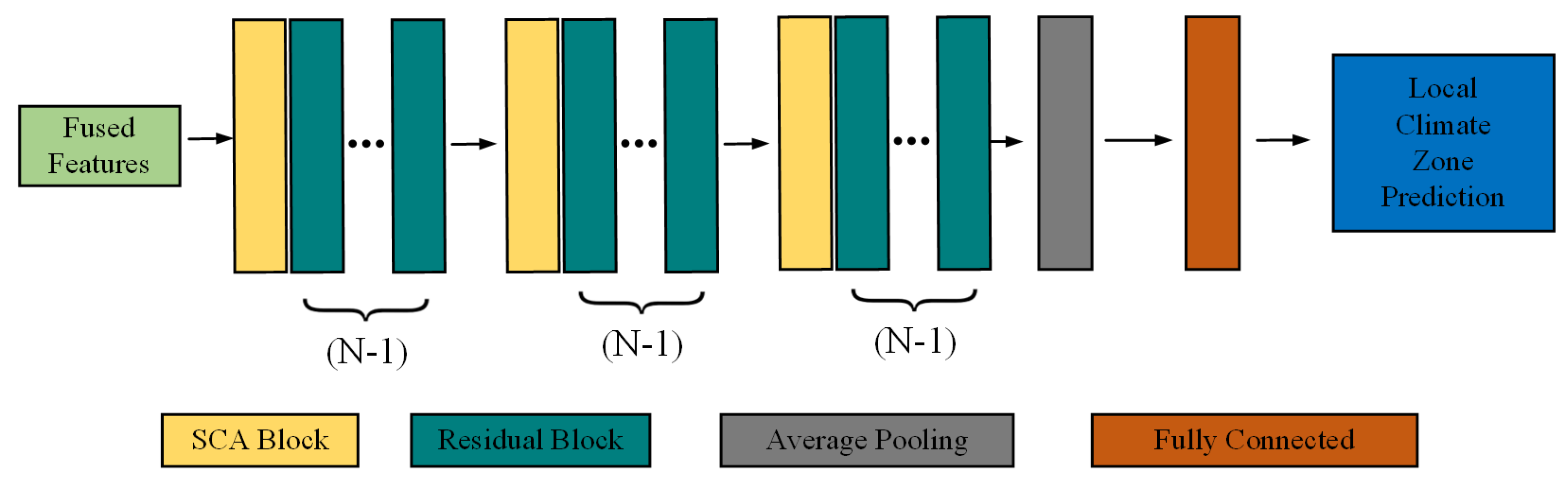
- A multi-branch fusion CNN is proposed to perform LCZ classification, where a multi-branch structure is introduced to extract and fuse features, with residual learning and self channel attention combined into the proposed classifier to accomplish the LCZ mapping.
- (3)
- We conducted experiments on the So2Sat LCZ42 dataset as well as real scenarios, and the experimental results demonstrate the effectiveness and robustness of our proposed method.
2. Related Work
3. Methodology
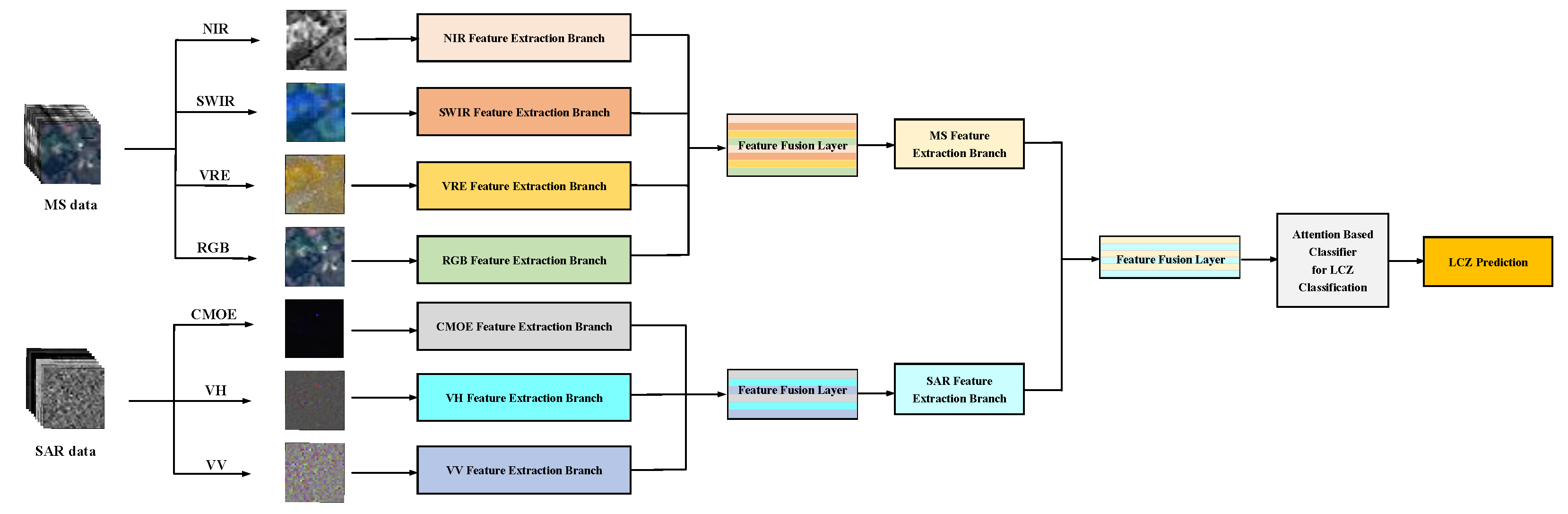
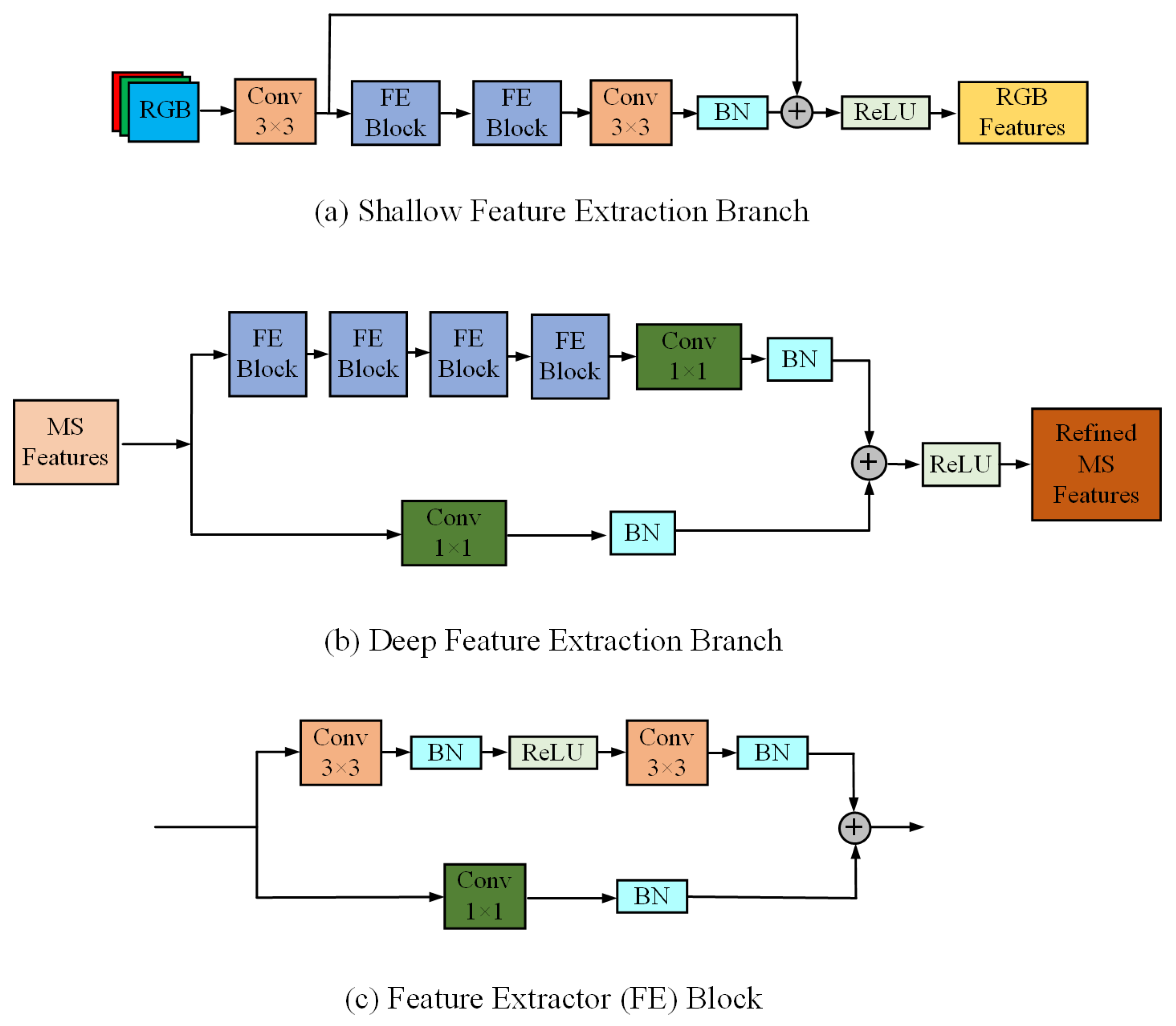
3.1. Multi-Branch CNN for Feature Fusion
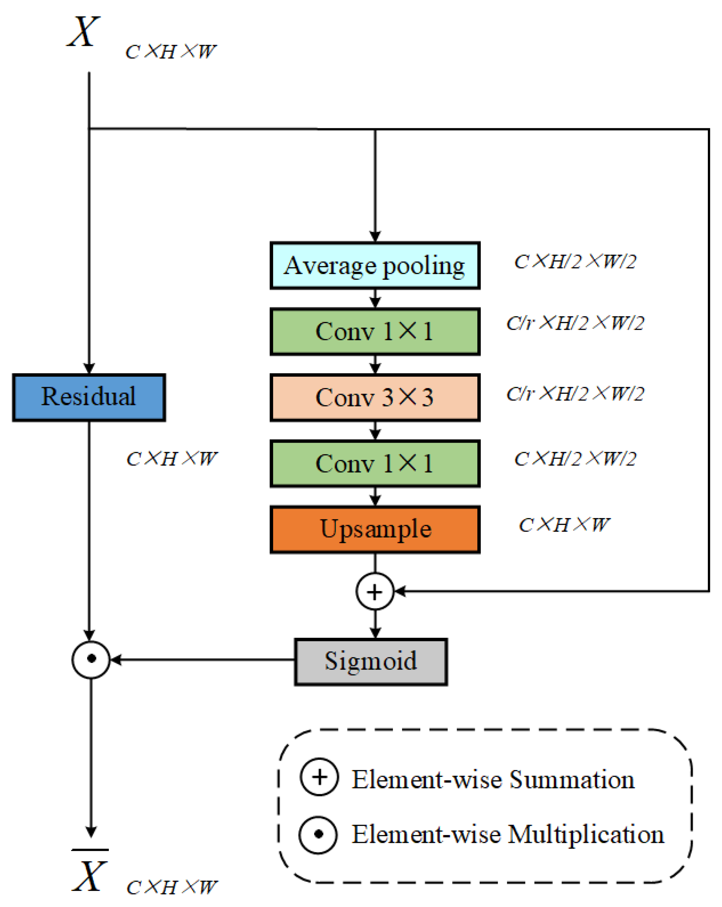
3.2. Self Channel Attention for LCZ Classification
4. Experiments
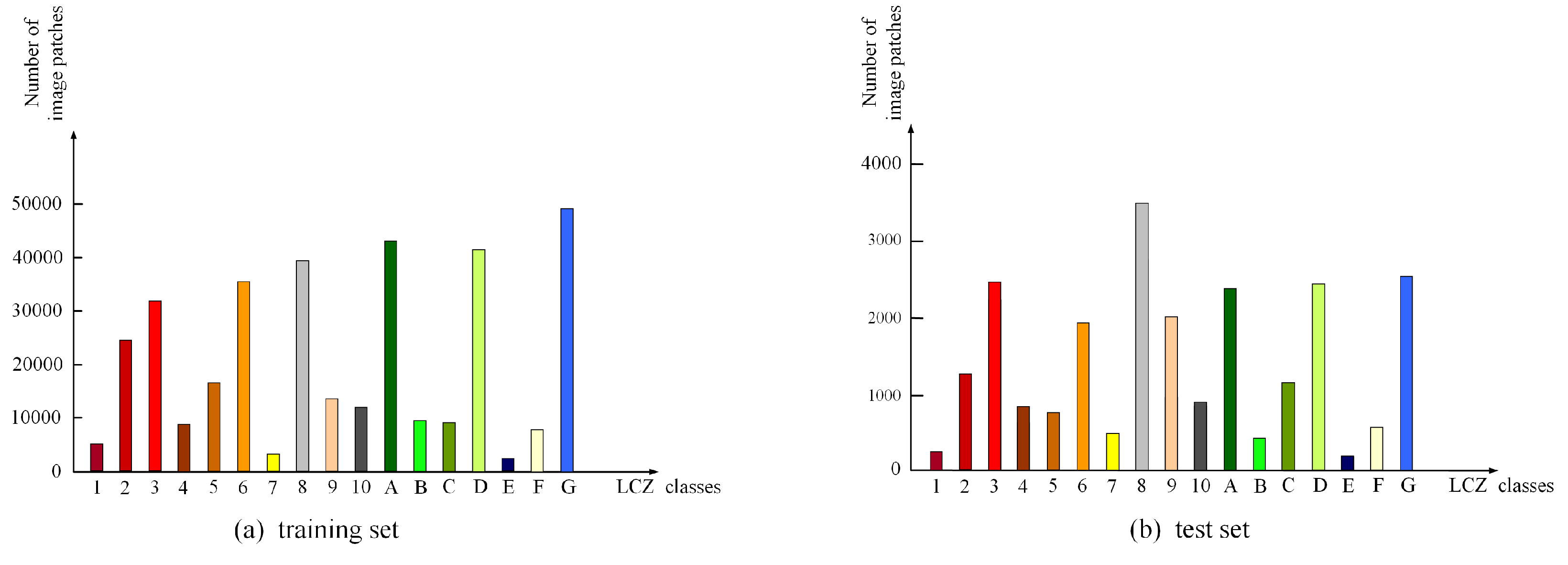
4.1. Dataset
4.2. Experimental Setup
4.3. Performance Metrics
4.4. Performance Evaluation
4.5. Performance Comparison with State-of-the-Art Methods
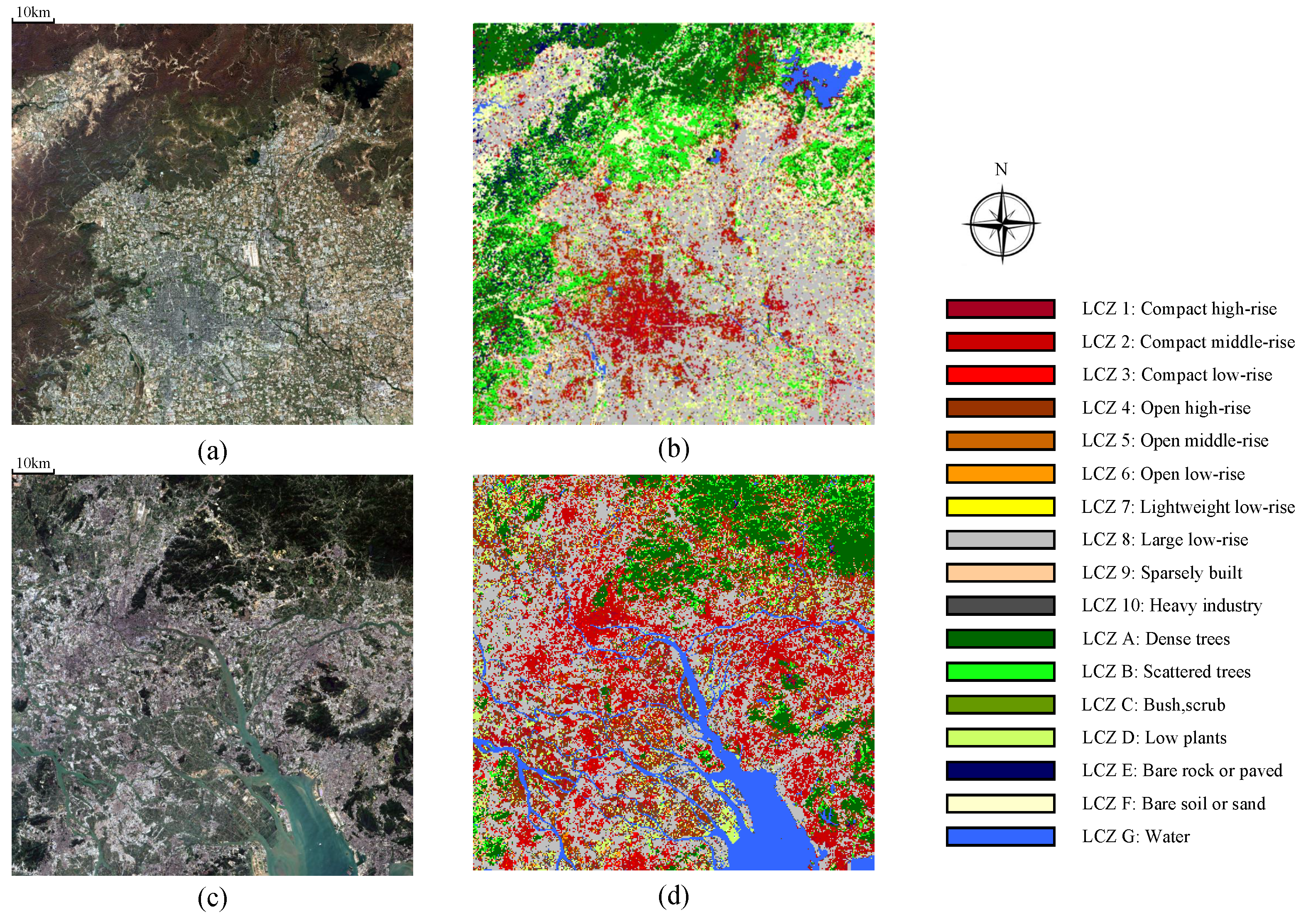
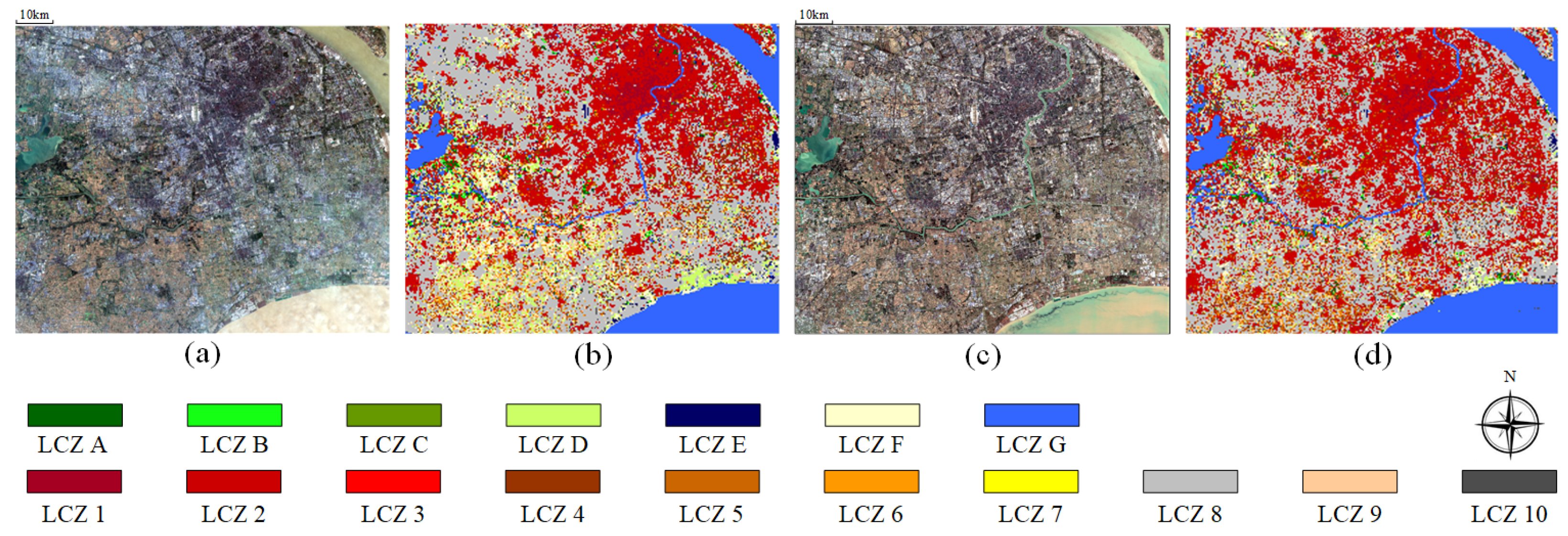
4.6. Large-Scale LCZ Maps
5. Discussion
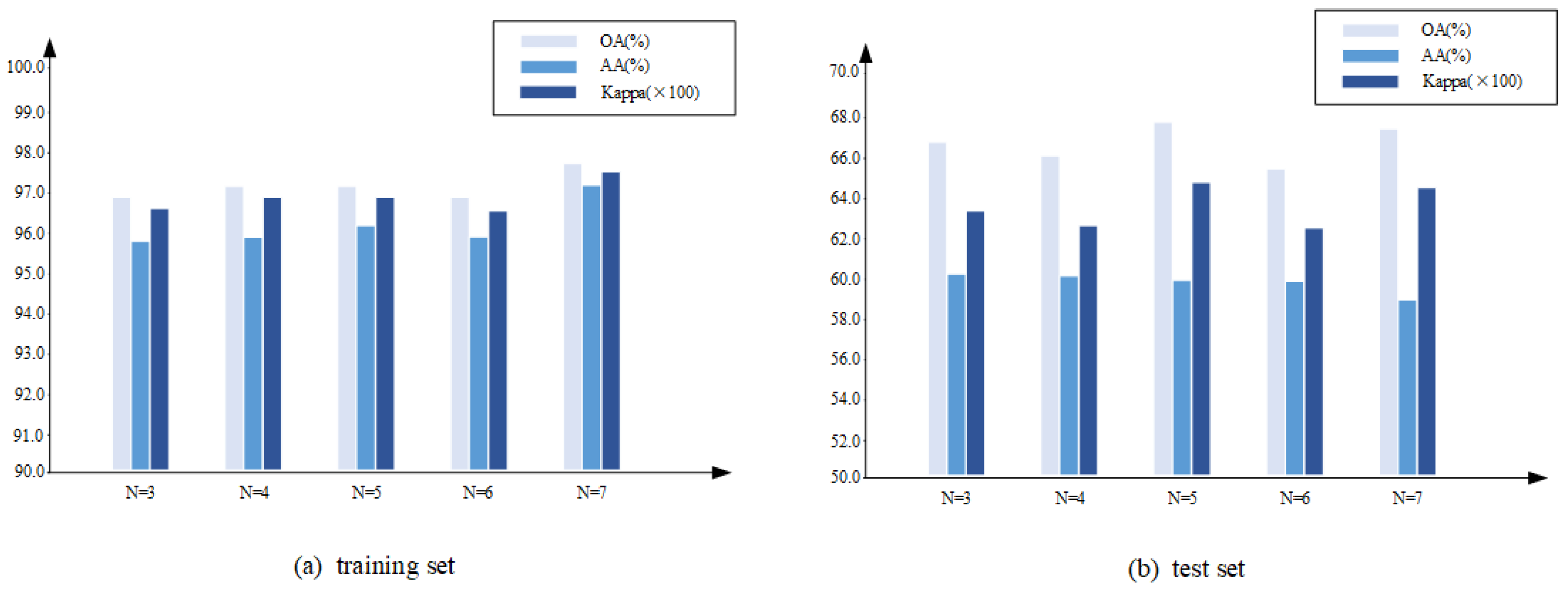
5.1. Effect of Network Depth
5.2. Effect of Data Fusion
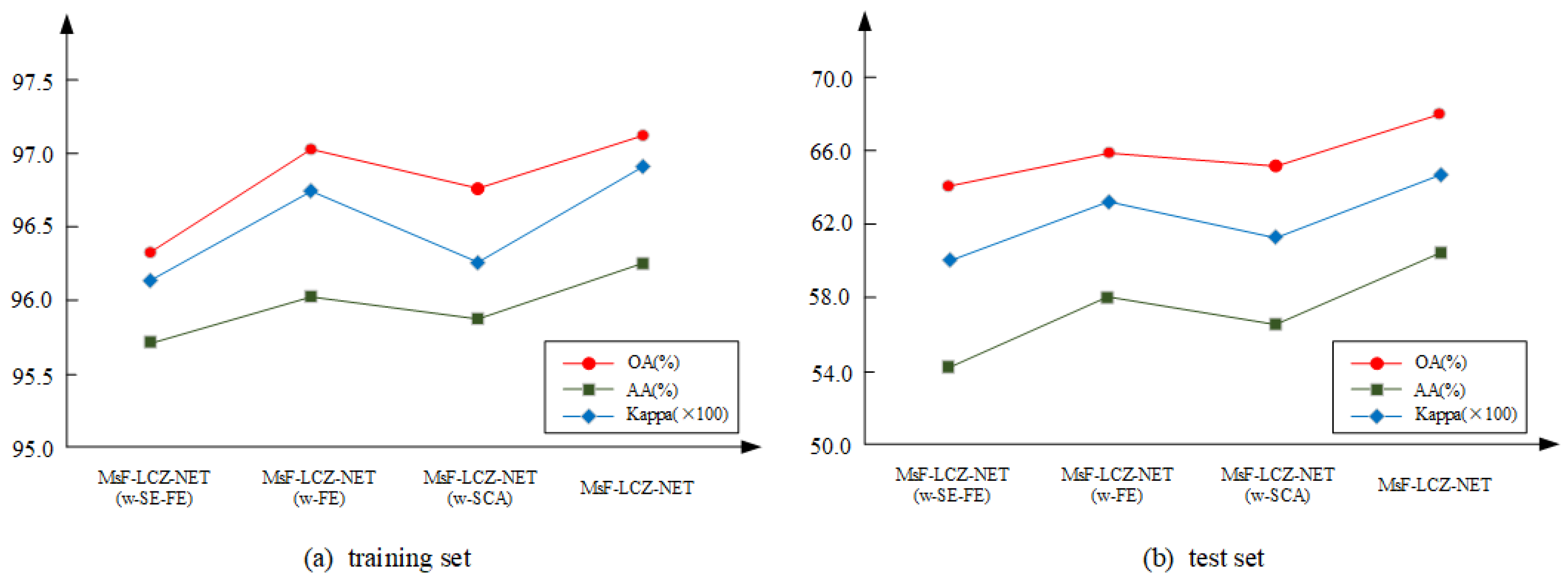
5.3. Ablation Study
6. Conclusions
Author Contributions
Funding
Institutional Review Board Statement
Informed Consent Statement
Data Availability Statement
Conflicts of Interest
References
- Kotharkar, R.; Bagade, A. Evaluating urban heat island in the critical local climate zones of an Indian city. Landsc. Urban Plan. 2018, 169, 92–104. [Google Scholar] [CrossRef]
- Stewart, I.D.; Oke, T.R. Local Climate Zones for Urban Temperature Studies. Bull. Am. Meteorol. Soc. 2012, 93, 1879–1900. [Google Scholar] [CrossRef]
- Alexandri, E.; Jones, P. Temperature decreases in an urban canyon due to green walls and green roofs in diverse climates. Build. Environ. 2008, 43, 480–493. [Google Scholar] [CrossRef]
- de Munck, C.; Pigeon, G.; Masson, V.; Meunier, F.; Bousquet, P.; Tréméac, B.; Merchat, M.; Poeuf, P.; Marchadier, C. How much can air conditioning increase air temperatures for a city like Paris, France? Int. J. Climatol. 2013, 33, 210–227. [Google Scholar] [CrossRef]
- Bechtel, B.; Daneke, C. Classification of local climate zones based on multiple earth observation data. IEEE J. Sel. Top. Appl. Earth Obs. Remote. Sens. 2012, 5, 1191–1202. [Google Scholar] [CrossRef]
- Xu, Y.; Ren, C.; Cai, M.; Wang, R. Issues and challenges of remote sensing-based local climate zone mapping for high-density cities. In Proceedings of the 2017 Joint Urban Remote Sensing Event (JURSE), Dubai, United Arab Emirates, 6–8 March 2017; pp. 1–4. [Google Scholar]
- Schmitt, M.; Hughes, L.; Zhu, X.X. The SEN1-2 dataset for deep learning in SAR-optical data fusion. ISPRS Ann. Photogramm. Remote Sens. Spat. Inf. Sci. 2018, 4, 141–146. [Google Scholar] [CrossRef] [Green Version]
- Mills, G.; Ching, J.; See, L.; Bechtel, B.; Foley, M. An introduction to the WUDAPT project. In Proceedings of the the 9th International Conference on Urban Climate, Toulouse, France, 20–24 July 2015; pp. 20–24. [Google Scholar]
- Bechtel, B.; Foley, M.; Mills, G.; Ching, J.; See, L.; Alexander, P.; O’Connor, M.; Albuquerque, T.; de Fatima Andrade, M.; Brovelli, M.; et al. CENSUS of Cities: LCZ Classification of Cities (Level 0)—Workflow and Initial Results From Various Cities. In Proceedings of the ICUC9-9th International Conference on Urban Climate Jointly with 12th Symposium on the Urban Environment, Toulouse, France, 20–24 July 2015. [Google Scholar]
- Seo, D.; Kim, Y.; Eo, Y.; Lee, M.; Park, W. Fusion of SAR and Multispectral Images Using Random Forest Regression for Change Detection. ISPRS Int. J.-Geo-Inf. 2018, 7, 401. [Google Scholar] [CrossRef] [Green Version]
- Oliver, C.; Quegan, S. Understanding Synthetic Aperture Radar Images; SciTech Publishing: Raleigh, NC, USA, 2004. [Google Scholar]
- Blaes, X.; Vanhalle, L.; Defourny, P. Efficiency of crop identification based on optical and SAR image time series. Remote. Sens. Environ. 2005, 96, 352–365. [Google Scholar] [CrossRef]
- Xu, G.; Zhu, X.; Tapper, N.; Bechtel, B. Urban climate zone classification using convolutional neural network and ground-level images. Prog. Phys. Geogr. Earth Environ. 2019, 43, 410–424. [Google Scholar] [CrossRef]
- Hong, G.; Zhang, Y.; Mercer, B. A wavelet and IHS integration method to fuse high resolution SAR with moderate resolution multispectral images. Photogramm. Eng. Remote Sens. 2009, 75, 1213–1223. [Google Scholar] [CrossRef]
- Liu, G.; Li, L.; Gong, H.; Jin, Q.; Li, X.; Song, R.; Chen, Y.; Chen, Y.; He, C.; Huang, Y.; et al. Multisource remote sensing imagery fusion scheme based on bidimensional empirical mode decomposition (BEMD) and its application to the extraction of bamboo forest. Remote. Sens. 2016, 9, 19. [Google Scholar] [CrossRef] [Green Version]
- He, K.; Zhang, X.; Ren, S.; Jian, S. Identity Mappings in Deep Residual Networks. In Proceedings of the European Conference on Computer Vision, Amsterdam, The Netherlands, 11–14 October 2016. [Google Scholar]
- Chunping, Q.; Schmitt, M.; Lichao, M.; Xiaoxiang, Z. Urban local climate zone classification with a residual convolutional neural network and multi-seasonal Sentinel-2 images. In Proceedings of the 2018 10th IAPR Workshop on Pattern Recognition in Remote Sensing (PRRS), Beijing, China, 19–20 August 2018; pp. 1–5. [Google Scholar]
- Qiu, C.; Tong, X.; Schmitt, M.; Bechtel, B.; Zhu, X.X. Multilevel Feature Fusion-based CNN for Local Climate Zone Classification from Sentinel-2 Images: Benchmark Results on the So2Sat LCZ42 Dataset. IEEE J. Sel. Top. Appl. Earth Obs. Remote Sens. 2020, 13, 2793–2806. [Google Scholar] [CrossRef]
- Zhou, Y.; Wei, T.; Zhu, X.; Collin, M. A Parcel-Based Deep-Learning Classification to Map Local Climate Zones From Sentinel-2 Images. IEEE J. Sel. Top. Appl. Earth Obs. Remote. Sens. 2021, 14, 4194–4204. [Google Scholar] [CrossRef]
- Yang, R.; Zhang, Y.; Zhao, P.; Ji, Z.; Deng, W. MSPPF-Nets: A Deep Learning Architecture for Remote Sensing Image Classification. In Proceedings of the IGARSS 2019 IEEE International Geoscience and Remote Sensing Symposium, Yokohama, Japan, 28 July–2 August 2019; pp. 3045–3048. [Google Scholar]
- Fiaschi, S.; Holohan, E.P.; Sheehy, M.; Floris, M. PS-InSAR analysis of Sentinel-1 data for detecting ground motion in temperate oceanic climate zones: A case study in the Republic of Ireland. Remote Sens. 2019, 11, 348. [Google Scholar] [CrossRef] [Green Version]
- Bechtel, B.; See, L.; Mills, G.; Foley, M. Classification of local climate zones using SAR and multispectral data in an arid environment. IEEE J. Sel. Top. Appl. Earth Obs. Remote Sens. 2016, 9, 3097–3105. [Google Scholar] [CrossRef]
- Shi, L.; Ling, F. Local Climate Zone Mapping Using Multi-Source Free Available Datasets on Google Earth Engine Platform. Land 2021, 10, 454. [Google Scholar] [CrossRef]
- Yan, Z.; Ma, L.; He, W.; Zhou, L.; Lu, H.; Liu, G.; Huang, G. Comparing Object-Based and Pixel-Based Methods for Local Climate Zones Mapping with Multi-Source Data. Remote Sens. 2022, 14, 3744. [Google Scholar] [CrossRef]
- Feng, P.; Lin, Y.; Guan, J.; Dong, Y.; He, G.; Xia, Z.; Shi, H. Embranchment CNN Based Local Climate Zone Classification Using Sar And Multispectral Remote Sensing Data. In Proceedings of the IGARSS 2019 IEEE International Geoscience and Remote Sensing Symposium, Yokohama, Japan, 28 July–2 August 2019; pp. 6344–6347. [Google Scholar]
- Feng, P.; Lin, Y.; He, G.; Guan, J.; Wang, J.; Shi, H. A Dynamic End-to-End Fusion Filter for Local Climate Zone Classification Using SAR and Multi-Spectrum Remote Sensing Data. In Proceedings of the IGARSS 2020—2020 IEEE International Geoscience and Remote Sensing Symposium, Waikoloa, HI, USA, 26 September–2 October 2020; pp. 4231–4234. [Google Scholar]
- Hu, J.; Shen, L.; Sun, G. Squeeze-and-excitation networks. In Proceedings of the the IEEE Conference on Computer Vision and Pattern Recognition, Salt Lake City, UT, USA, 18–23 June 2018; pp. 7132–7141. [Google Scholar]
- Zhu, X.X.; Hu, J.; Qiu, C.; Shi, Y.; Kang, J.; Mou, L.; Bagheri, H.; Haberle, M.; Hua, Y.; Huang, R.; et al. So2Sat LCZ42: A benchmark data set for the classification of global local climate zones [Software and Data Sets]. IEEE Geosci. Remote Sens. Mag. 2020, 8, 76–89. [Google Scholar] [CrossRef] [Green Version]
- Bechtel, B.; Alexander, P.J.; Beck, C.; Böhner, J.; Brousse, O.; Ching, J.; Demuzere, M.; Fonte, C.; Gál, T.; Hidalgo, J.; et al. Generating WUDAPT Level 0 data–Current status of production and evaluation. Urban Clim. 2019, 27, 24–45. [Google Scholar] [CrossRef] [Green Version]
- Kingma, D.P.; Ba, J. Adam: A method for stochastic optimization. In Proceedings of the International Conference on Learning Representations (ICLR), San Diego, CA, USA, 7–9 May 2015; pp. 1–13. [Google Scholar]
- Fu, J.; Liu, J.; Tian, H.; Li, Y.; Bao, Y.; Fang, Z.; Lu, H. Dual attention network for scene segmentation. In Proceedings of the IEEE Conference on Computer Vision and Pattern Recognition, Long Beach, CA, USA, 15–20 June 2019; pp. 3146–3154. [Google Scholar]
- AlBeladi, A.A.; Muqaibel, A.H. Evaluating compressive sensing algorithms in through-the-wall radar via F1-score. Int. J. Signal Imaging Syst. Eng. 2018, 11, 164–171. [Google Scholar] [CrossRef]
- McHugh, M.L. Interrater reliability: The kappa statistic. Biochem. Med. Biochem. Med. 2012, 22, 276–282. [Google Scholar] [CrossRef]
- Gawlikowski, J.; Schmitt, M.; Kruspe, A.; Zhu, X.X. On the fusion strategies of Sentinel-1 and Sentinel-2 data for local climate zone classification. In Proceedings of the IGARSS 2020—2020 IEEE International Geoscience and Remote Sensing Symposium, Waikoloa, HI, USA, 26 September–2 October 2020; pp. 2081–2084. [Google Scholar]
- Liu, S.; Shi, Q. Local climate zone mapping as remote sensing scene classification using deep learning: A case study of metropolitan China. ISPRS J. Photogramm. Remote Sens. 2020, 164, 229–242. [Google Scholar] [CrossRef]
- Ji, W.; Chen, Y.; Li, K.; Dai, X. Multicascaded Feature Fusion-Based Deep Learning Network for Local Climate Zone Classification Based on the So2Sat LCZ42 Benchmark Dataset. IEEE J. Sel. Top. Appl. Earth Obs. Remote Sens. 2022, 16, 449–467. [Google Scholar] [CrossRef]
- Zhou, L.; Shao, Z.; Wang, S.; Huang, X. Deep learning-based local climate zone classification using Sentinel-1 SAR and Sentinel-2 multispectral imagery. Geo-Spat. Inf. Sci. 2022, 25, 1–16. [Google Scholar] [CrossRef]
- Chang, J.G.; Shoshany, M.; Oh, Y. Polarimetric radar vegetation index for biomass estimation in desert fringe ecosystems. IEEE Trans. Geosci. Remote Sens. 2018, 56, 7102–7108. [Google Scholar] [CrossRef]


| Number | Band | Number | Band |
|---|---|---|---|
| 1st band | Real part of the unfiltered VH channel | 9th band | B2 |
| 2nd band | Imaginary part of the unfiltered VH channel | 10th band | B3 |
| 3rd band | Real part of the unfiltered VV channel | 11th band | B4 |
| 4th band | Imaginary part of the unfiltered VV channel | 12th band | B5 (upsampled to 10 m from 20 m GSD) |
| 5th band | Intensity of the refined Lee-filtered VH signal | 13th band | B6 (upsampled to 10 m from 20 m GSD) |
| 6th band | Intensity of the refined Lee-filtered VV signal | 14th band | B7 (upsampled to 10 m from 20 m GSD) |
| 7th band | Real part of the refined Lee-filtered covariance matrix off-diagonal element | 15th band 16th band | B8 B8a (upsampled to 10 m from 20 m GSD) |
| 8th band | Imaginary part of the refined Lee-filtered covariance matrix off-diagonal element | 17th band 18th band | B11 (upsampled to 10 m from 20 m GSD) B12 (upsampled to 10 m from 20 m GSD) |
| Group | Band | Group | Band |
|---|---|---|---|
| VV | 1st band 2nd band 5th band | RGB | 9th band 10th band 11th band |
| VH | 3rd band 4th band 6th band | VRE | 12th band 13th band 14th band 16th band |
| CMOE | 7th band 8th band | SWIR | 17th band 18th band |
| NIR | 15th band |
| Class | (%) | |||
|---|---|---|---|---|
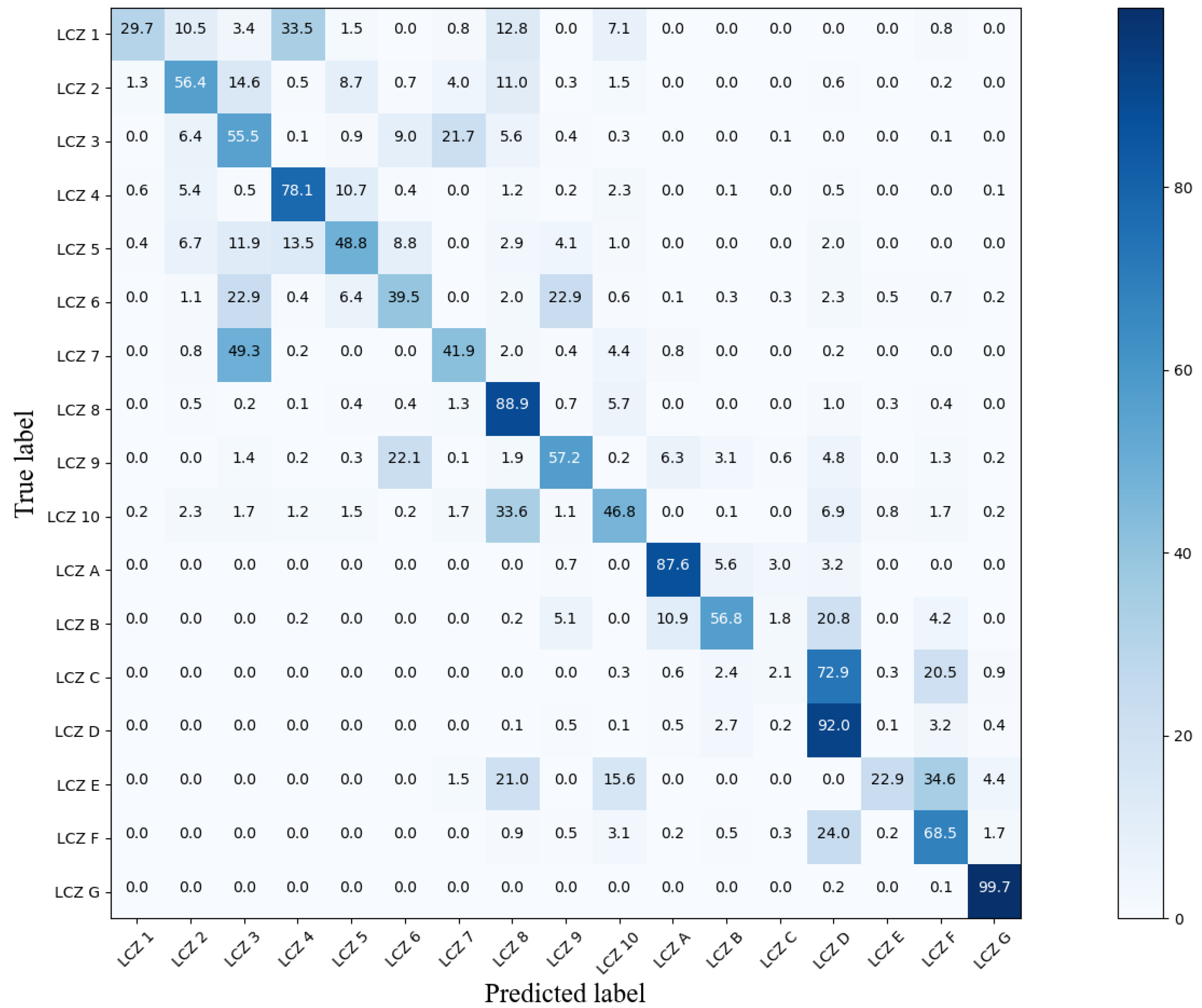
| LCZ 1: compact high-rise | 29.7 | 74.5 | 42.5 | 1.44 |
| LCZ 2: compact mid-rise | 56.4 | 67.1 | 61.3 | 6.93 |
| LCZ 3: compact low-rise | 55.5 | 57.0 | 56.3 | 8.99 |
| LCZ 4: open high-rise | 78.1 | 74.5 | 76.2 | 2.46 |
| LCZ 5: open mid-rise | 48.8 | 49.1 | 48.9 | 4.68 |
| LCZ 6: open low-rise | 39.5 | 50.1 | 44.1 | 10.02 |
| LCZ 7: lightweight low-rise | 41.9 | 24.4 | 30.8 | 0.93 |
| LCZ 8: large low-rise | 88.9 | 79.8 | 84.1 | 11.16 |
| LCZ 9: sparsely built | 57.2 | 66.5 | 61.5 | 3.86 |
| LCZ 10: heavy industry | 46.8 | 53.7 | 50.0 | 3.39 |
| LCZ A: dense trees | 87.6 | 91.2 | 89.4 | 12.18 |
| LCZ B: scattered trees | 56.8 | 45.2 | 50.4 | 2.70 |
| LCZ C: bush and scrub | 2.1 | 18.2 | 3.7 | 2.60 |
| LCZ D: low plants | 92.0 | 61.1 | 73.5 | 11.74 |
| LCZ E: bare rock or paved | 22.9 | 57.3 | 32.8 | 0.68 |
| LCZ F: bare soil or sand | 68.5 | 44.6 | 54.1 | 2.24 |
| LCZ G: water | 99.7 | 98.1 | 98.9 | 14.00 |
| MSPPF-NETS [20] | 62.05 | 51.32 | 58.54 |
| LCZ-MF [18] | 65.66 | 50.63 | 62.21 |
| EB-CNN [25] | 61.11 | 44.37 | 57.07 |
| DenseNet-DFN [26] | 64.07 | 50.59 | 60.49 |
| FusionNet [34] | 64.57 | 52.17 | 57.45 |
| LCZNet [35] | 66.23 | 57.76 | 63.15 |
| ResNext29_8_64 [24] | 64.91 | 54.05 | 61.47 |
| MCFUNet-LCZ [36] | 65.74 | 53.18 | 61.94 |
| RSNNet [37] | 64.15 | 51.66 | 60.79 |
| MsF-LCZ-Net (N = 5) | 67.87 | 59.56 | 64.76 |
| Dataset | OA (%) | AA (%) | Kappa (×100) |
|---|---|---|---|
| SAR | 32.08 | 22.14 | 26.54 |
| SAR(Lee-filtered) | 46.74 | 39.75 | 41.37 |
| MS | 65.41 | 53.96 | 60.72 |
| MS & SAR | 67.87 | 59.56 | 64.76 |
| MS & SAR(Lee-filtered) | 68.02 | 60.27 | 65.15 |
Disclaimer/Publisher’s Note: The statements, opinions and data contained in all publications are solely those of the individual author(s) and contributor(s) and not of MDPI and/or the editor(s). MDPI and/or the editor(s) disclaim responsibility for any injury to people or property resulting from any ideas, methods, instructions or products referred to in the content. |
© 2023 by the authors. Licensee MDPI, Basel, Switzerland. This article is an open access article distributed under the terms and conditions of the Creative Commons Attribution (CC BY) license (https://creativecommons.org/licenses/by/4.0/).
Share and Cite
He, G.; Dong, Z.; Guan, J.; Feng, P.; Jin, S.; Zhang, X. SAR and Multi-Spectral Data Fusion for Local Climate Zone Classification with Multi-Branch Convolutional Neural Network. Remote Sens. 2023, 15, 434. https://doi.org/10.3390/rs15020434
He G, Dong Z, Guan J, Feng P, Jin S, Zhang X. SAR and Multi-Spectral Data Fusion for Local Climate Zone Classification with Multi-Branch Convolutional Neural Network. Remote Sensing. 2023; 15(2):434. https://doi.org/10.3390/rs15020434
Chicago/Turabian StyleHe, Guangjun, Zhe Dong, Jian Guan, Pengming Feng, Shichao Jin, and Xueliang Zhang. 2023. "SAR and Multi-Spectral Data Fusion for Local Climate Zone Classification with Multi-Branch Convolutional Neural Network" Remote Sensing 15, no. 2: 434. https://doi.org/10.3390/rs15020434