Orbital Uncertainty Propagation Based on Adaptive Gaussian Mixture Model under Generalized Equinoctial Orbital Elements

Abstract

The number of resident space objects (RSOs) has been steadily increasing over time, posing significant risks to the safe operation of on-orbit assets. The accurate prediction of potential collision events and implementation of effective and nonredundant avoidance maneuvers require the precise estimation of the orbit positions of objects of interest and propagation of their associated uncertainties. Previous research mainly focuses on striking a balance between accurate propagation and efficient computation. A recently proposed approach that integrates uncertainty propagation with different coordinate representations has the potential to achieve such a balance. This paper proposes combining the generalized equinoctial orbital elements (GEqOE) representation with an adaptive Gaussian mixture model (GMM) for uncertainty propagation. Specifically, we implement a reformulation for the orbital dynamics so that the underlying state and the moment feature of the GMM are propagated under the GEqOE coordinates. Starting from an initial Gaussian probability distribution function (PDF), the algorithm iteratively propagates the uncertainty distribution using a detection-splitting module. A differential entropy-based nonlinear detector and a splitting library are utilized to adjust the number of GMM components dynamically. Component splitting is triggered when a predefined threshold of differential entropy is violated, generating several GMM components. The final probability density function (PDF) is obtained by a weighted summation of the component distributions at the target time. Benefiting from the nonlinearity reduction caused by the GEqOE representation, the number of triggered events largely decreases, causing the necessary number of components to maintain uncertainty realism also to decrease, which enables the proposed approach to achieve good performance with much more efficiency. As demonstrated by the results of propagation in three scenarios with different degrees of complexity, compared with the Cartesian-based approach, the proposed approach achieves comparable accuracy to the Monte Carlo method while largely reducing the number of components generated during propagation. Our results confirm that a judicious choice of coordinate representation can significantly improve the performance of uncertainty propagation methods in terms of accuracy and computational efficiency.

1. Introduction

The increasing number of space targets poses a great risk to the safe operation of on-orbit assets. The accurate location and prediction of objects of interest are crucial for enhancing space situational awareness. Currently, both ground-based and space-based observation systems face challenges in meeting the demanding monitoring requirements of the numerous targets due to their limited capabilities. As a result, there is a scarcity of orbital geometry information from sparse measurements. Furthermore, the observation arcs and the considered dynamical model used as inputs in the orbit determination algorithm have limited accuracy. All of these factors contribute to orbit uncertainty, which represents the deviation between the estimated and actual orbits. In specific applications, solely predicting the nominal orbit is inadequate, as considering the evolution of uncertainty is also critical. This is particularly true in scenarios where mission reliability is of paramount concern, such as spacecraft constellation configuration [1,2], space rendezvous [3], and collision assessment [4].

Uncertainty in a dynamical system primarily refers to both the inherent stochastic term and the epistemic uncertainty in modeling. It is typically associated with errors in algorithms for orbit computation, modeling defects caused by forces, and measurement noise, ultimately resulting in orbital uncertainty. The output of the orbit determination pipeline is often characterized as a Gaussian probability density function (PDF), which serves as input for the procedure of uncertainty propagation (UP). The evolution of the uncertainty PDF is governed by the Fokker–Planck (FP) equation [5], and obtaining an analytical solution to the FP partial differential equation (PDE) can be challenging, while numerical calculations are extremely time-consuming. The Monte Carlo method, a sampling-based approach, is an accurate and effective technique for uncertainty propagation [6]. However, mapping numerous samples for reliable analysis can be also computationally intensive. In practice, it is typically used as a quantitative benchmark in uncertainty propagation methods. Currently, many techniques have been developed to propagate uncertainty accurately and efficiently [7], falling into two categories: intrusive and nonintrusive methods.

The intrusive method employs an approximate dynamic model to simplify the propagation of the distribution over time. The dynamical system is represented during the analysis as a Taylor series expansion around the nominal orbit. Based on the chosen approximate order of the model, the uncertainty propagation method can be categorized into two classes: the linear covariance analysis (LinCov) method [8], which depends on the first-order state transition matrix (STM), and the state transition tensors (STT) method [9], which preserves the high-order nonlinear term. Under the LinCov method, the Gaussian PDF is used to fully characterize the underlying uncertainty. However, this method may become inaccurate when dealing with highly nonlinear dynamics or when uncertainties distort significantly after long-term propagation. On the other hand, STT improves upon the traditional linearized method by utilizing the high-order terms in the Taylor expansion to handle nonlinearity in dynamics, providing an advantage for reliable uncertainty propagation. Nonetheless, STT highly depends on the propagation of the high-order variational equation, increasing its computational requirements exponentially as the maximum order of STT considered increases. The differential algebra-based method [3] also uses Taylor polynomials to expand the dynamics. Instead of integrating variational equations, differential algebra employs an algebraic approach over these Taylor polynomials to automatically map the initial conditions with the solution of complicated equations, allowing for more efficient propagation compared to STT. It is important to note that Taylor expansion represents a local solution in the neighborhoods of the nominal trajectory. Depending on the nonlinearity of the dynamics, the size of the initial uncertainty, and the propagation time, the Taylor expansion needs to be dynamically adapted to achieve the required accuracy. Techniques like automatic domain splitting (ADS) [3] and lower-order automatic domain splitting (LOADS) [10] are employed to address this challenge.

Nonintrusive methods present another sampling-based approach, but they pursue deterministic sampling to efficiently propagate the initial distribution. One classical nonintrusive approach is the unscented transform (UT) [11], commonly used to propagate the first two statistical moments, i.e., mean and covariance, when dealing with Gaussian uncertainties. The second-order moment can be characterized by sampling and propagating a few sigma samples into future epochs. Similar numerical quadrature rules include the Gauss–Hermite quadrature (GHQ) [12], cubature rules (CRs) [13], and compact quadrature rules (CQRs) [14]. The UT and CRs both belong to third-degree rules, whereas the GHQ rule is accurate to arbitrary degrees, making it more suitable for propagating long-term means and covariances. However, it is worth noting that the GHQ rule requires univariate tensor product calculations, which can lead to the curse of dimensionality. In contrast, higher-degree CRs introduced in [15] have demonstrated comparable performance to GHQ but with a computational complexity on the order of polynomials of the dimension. When applying the UT and the high-degree CRs, it is essential to be mindful of the potential occurrence of negative quadrature weights, which can lead to a negative-definite covariance matrix and degrade propagation performance. To address this problem, Bin Jia and Ming Xin [14] proposed a new class of compact quadrature rules (CQRs) for the orbital uncertainty propagation based on two positive weighted quadrature rules from [16,17]. The CQRs offer similar performance to GHQ but require considerably fewer quadrature points. Another nonintrusive method is the polynomial chaos equation (PCE) method [18], which provides a functional approximation of the orbital dynamics through its spectral representation using orthonormal polynomials. Once the polynomial chaos coefficients are calculated, an inexpensive-to-evaluate surrogate is constructed to replace the underlying dynamical system, resulting in a final PDF recovered from the evaluated samples with less calculation compared to the MC method. However, it is important to note that the curse of dimensionality may arise when applying PCE in complex problems, as the number of terms required to construct the polynomial approximation grows exponentially with the dimension of the input variables and the order of the polynomial basis.

Many reviews of orbital uncertainty propagation methods reveal that the nonlinearity of dynamical partial differential equations significantly affects the performance of propagation methods [7,19]. As the initial Gaussian distribution propagates through nonlinear dynamics, it gradually deforms, making approaches relying on the assumption of a Gaussian PDF ineffective. One solution to this issue is to utilize the Gaussian mixture model (GMM) [20]. The GMM is an effective probability distribution model that characterizes any probability density function through a weighted sum of Gaussian components. Each component of the GMM has a smaller uncertainty, enabling the preservation of the effectiveness of the local linearization of the nonlinear function for a longer period within each Gaussian. By employing the divide-and-conquer strategy of the GMM, several approaches that depend on Gaussian validity have burst forth with new vitality, including GMM-UT [21,22], GMM-STT [23,24], GMM-DA [10,25], and GMM-PCE [26]. These approaches can be categorized into two classes. The first class aims to enhance their applicability in dealing with nonlinear dynamics. By dividing the large deviation into several smaller parts, the Gaussian validity is preserved for a longer period. As a result, the accuracy of deformed distribution descriptions is improved using methods that rely on Gaussian assumption, such as GMM-UT and linearization techniques. The second class aims to reduce the computational complexity of intrusive methods through GMM division. When handling uncertainty propagation, intrusive methods can replace the propagation flow within the component deviation domain with a lower-order surrogate model. The sum of all component surrogates can then be equivalent to a high-order propagation model corresponding to the original deviation domain, which significantly increases the computational efficiency of intrusive methods.

In addition, some strategies, such as the multifidelity model [27,28] and virtual sampling [29], are explored to achieve the balance of accuracy and efficiency of the GMM-based methods. However, when applying these GMM-based approaches to multivariate uncertainty propagation, the splitting operation along multiple dimensions leads to unbounded exploration of the component number, resulting in a degradation in execution efficiency. To address this issue, the Gaussian mixture reduction [30], including pruning [31] and merging operations [32] for GMM components, has been proposed to dynamically reduce the number of components, yielding some successful results. The pruning operation is to drop the components with the lowest probabilities, and it may reduce the accuracy of final results, while the number of Gaussian components is decreased gradually based on the probabilistic similarity measure. The similar components in the GMM would be merged to a single Gaussian component. Considering that the lack of established standards for triggering and executing GMM reduction makes it challenging to strike a balance between precision and efficiency during application, it is necessary to develop new strategies to tackle the propagation difficulty arising from nonlinear dynamics.

Recently, research on state representation has demonstrated its potential in mitigating the effects of nonlinearities on uncertainty propagation. The development of various element representations has usually been motivated by the goal of eliminating orbit singularities [33]. Remarkably, elegantly designed mathematical formulations can effectively absorb the dominant nonlinearity in the equations of motion (EOMs). For instance, coordinate systems based on orbital elements, such as the equinoctial orbital elements (EqOEs), can mitigate the nonlinear effect of the $1/r^2$ term in the geopotential [34]. Horwood et al. [19], in a significant advancement, replaced the semimajor axis of EqOEs with the mean motion, leading to the definition of the alternate set of elements (AEqOE). Using AEqOE, the Gaussianity of the initial state uncertainty can be preserved throughout its complete propagation in pure two-body dynamics. In consideration of perturbations on dynamics, Aristoff et al. [35] introduced a set of $J_2$ equinoctial orbital elements ($J_{2}EqOE$) that effectively absorb nonlinearities arising from the dominant $J_2$ term of the geopotential perturbation. Additionally, Baù et al. [36] proposed the generalized equinoctial orbital elements (GEqOE), which not only reduce the influence of the $J_2$ term but also address higher-order geopotential harmonics. Notably, Baù et al. [36] established a closed analytical transformation between Cartesian coordinates and GEqOE, along with a well-defined set of differential equations of motion. Furthermore, in [37], Javier et al. extended the research by computing the Jacobian matrix of the time derivatives of the GEqOE, thereby completing the representation of the motion with the GEqOE.

The effect of different state representations on mitigating the nonlinearity of the dynamics has been demonstrated in their original works [35,36,37]. However, the potential of these representations for uncertainty propagation remains to be explored. In this paper, we propose a reformulation of the GMM-UT method using the GEqOE representation for uncertainty propagation. Specifically, we express the orbital state and its distribution in the space of GEqOE and implement a GEqOE propagator to map the initial uncertainty to future epochs. To begin with, the initial Gaussian is approximated by a Gaussian mixture model, from which a set of sigma points is sampled to propagate the associated moment forward. An adaptive Gaussian mixture model based on differential entropy is used as the adaptive framework of the underlying PDF. When the differential entropy of a component exceeds a suitable threshold, a splitting operation is performed on the corresponding component. Benefiting from the preservation of Gaussianity under GeqOE, this paper achieves a reduction in the number of GMM components required for uncertainty realism, thereby enhancing the computation efficiency of GMM propagation. In summary, the main contributions of this paper are the following:

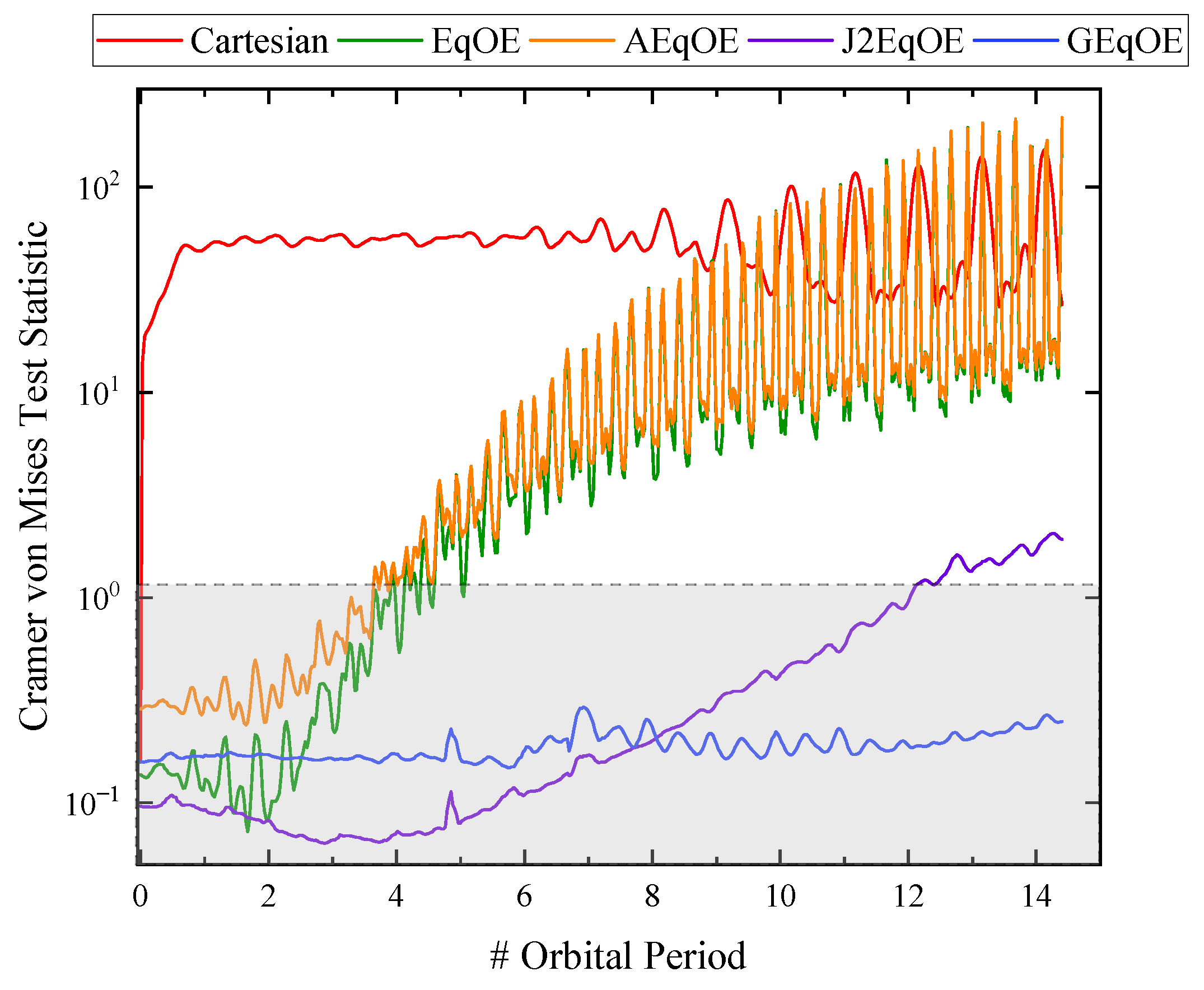
• This paper conducts a performance comparison of five orbital representations in mitigating dynamics nonlinearity during uncertainty propagation. The Cramer–von Mises test statistic demonstrates the excellence of the GEqOE representation in preserving uncertainty realism throughout propagation.
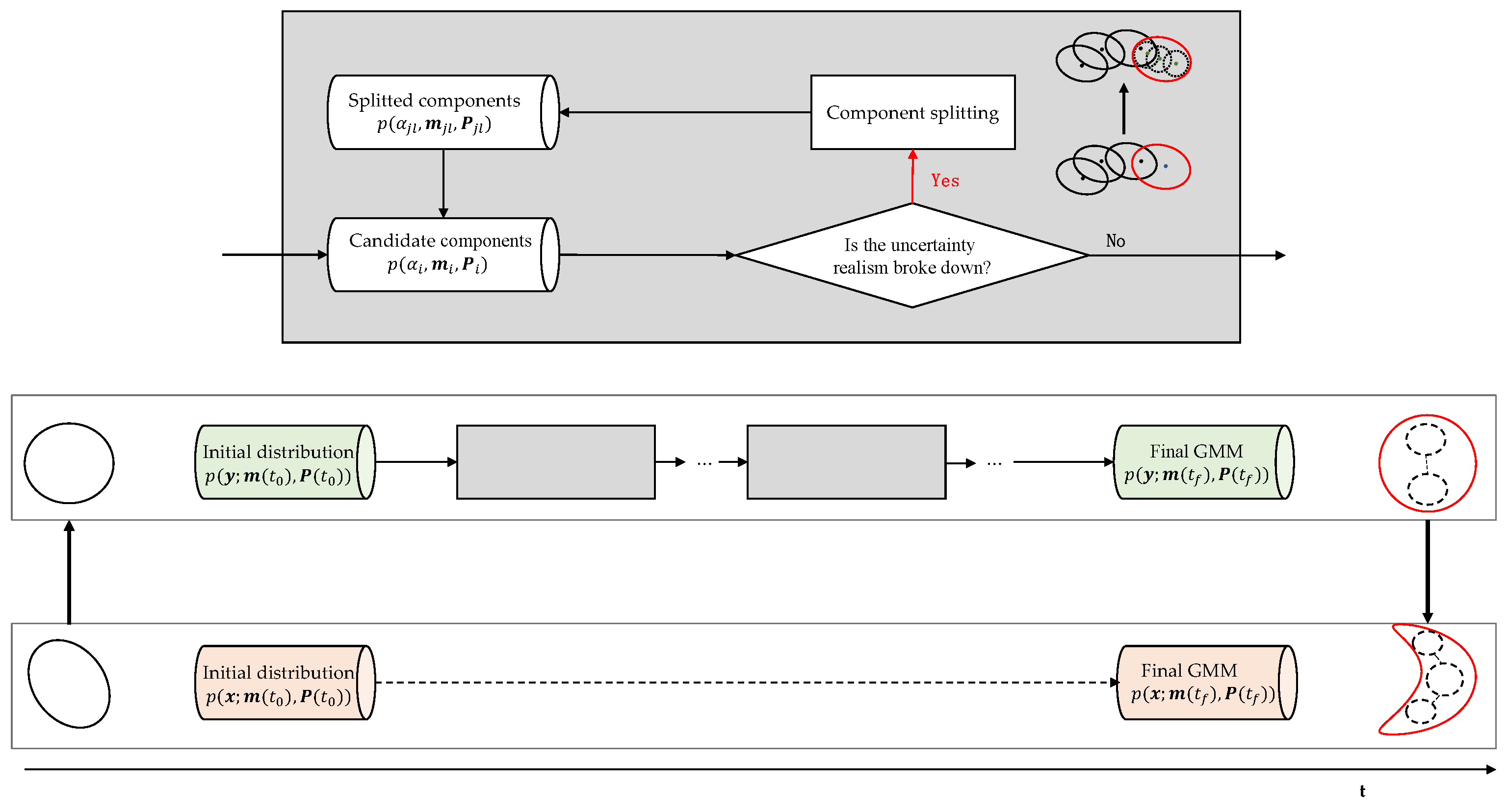
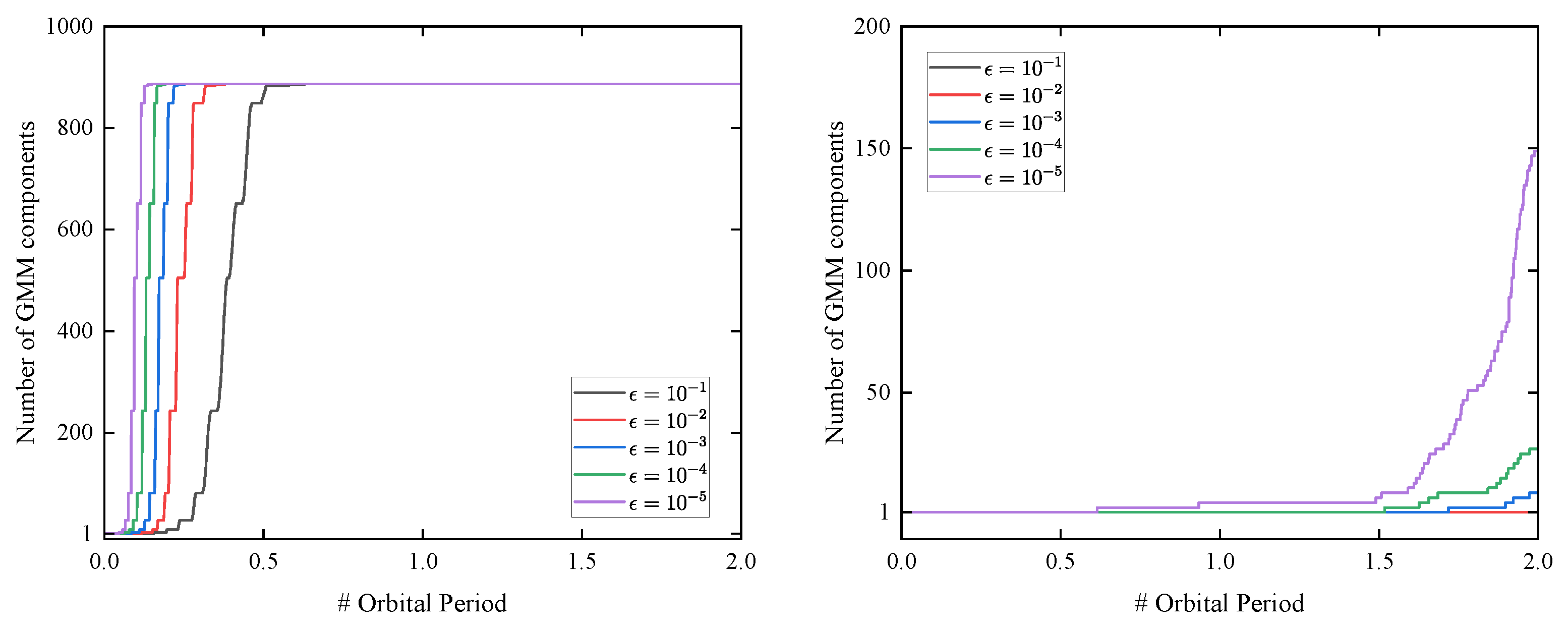
• This paper proposes an uncertainty propagation method named AEGIS-GEqOE, which combines the GMM strategy and the GEqOE state representation to efficiently and accurately propagate the uncertainty. The use of GEqOE allows us to reduce the number of GMM components required to describe the PDF of the propagated variables. Specifically, differential entropy-based splitting, designed to adaptively adjust the number of components, is applied with the GEqOE.
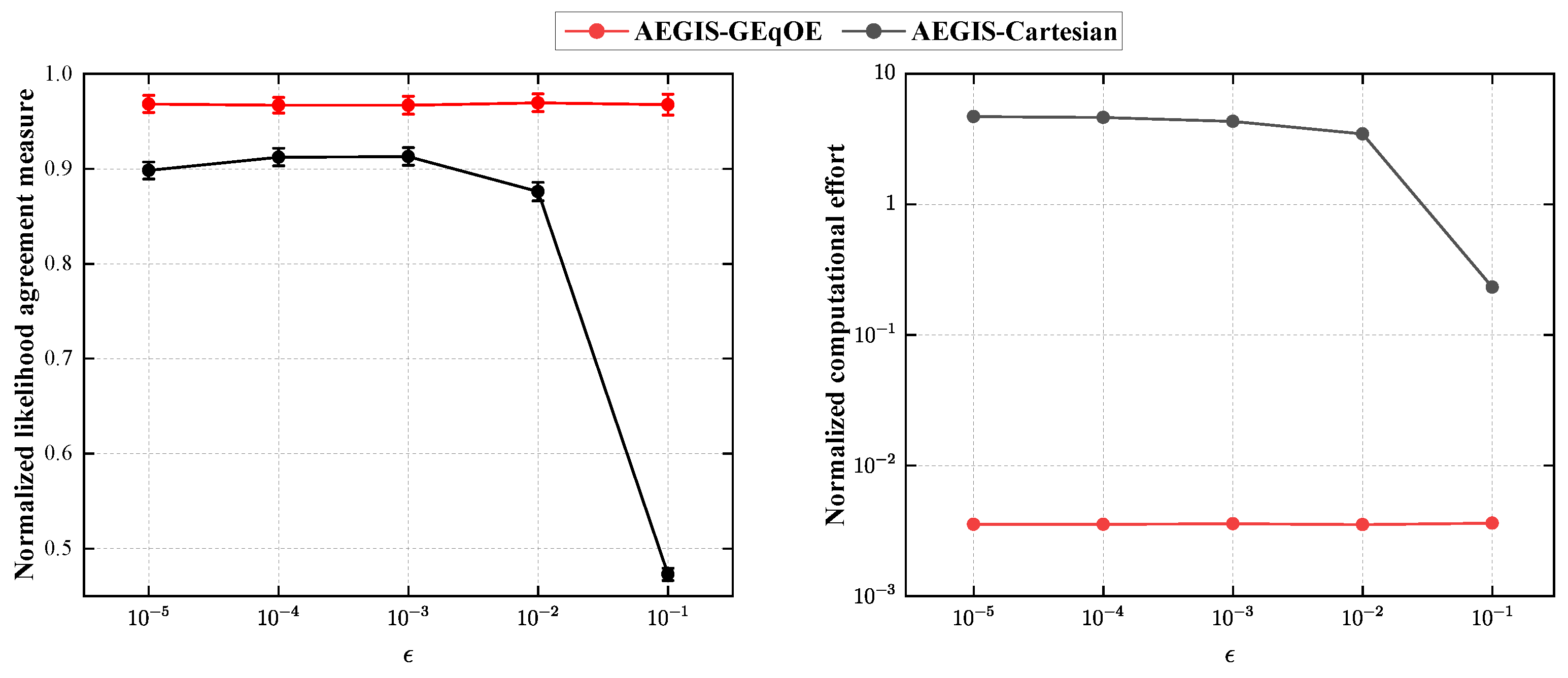
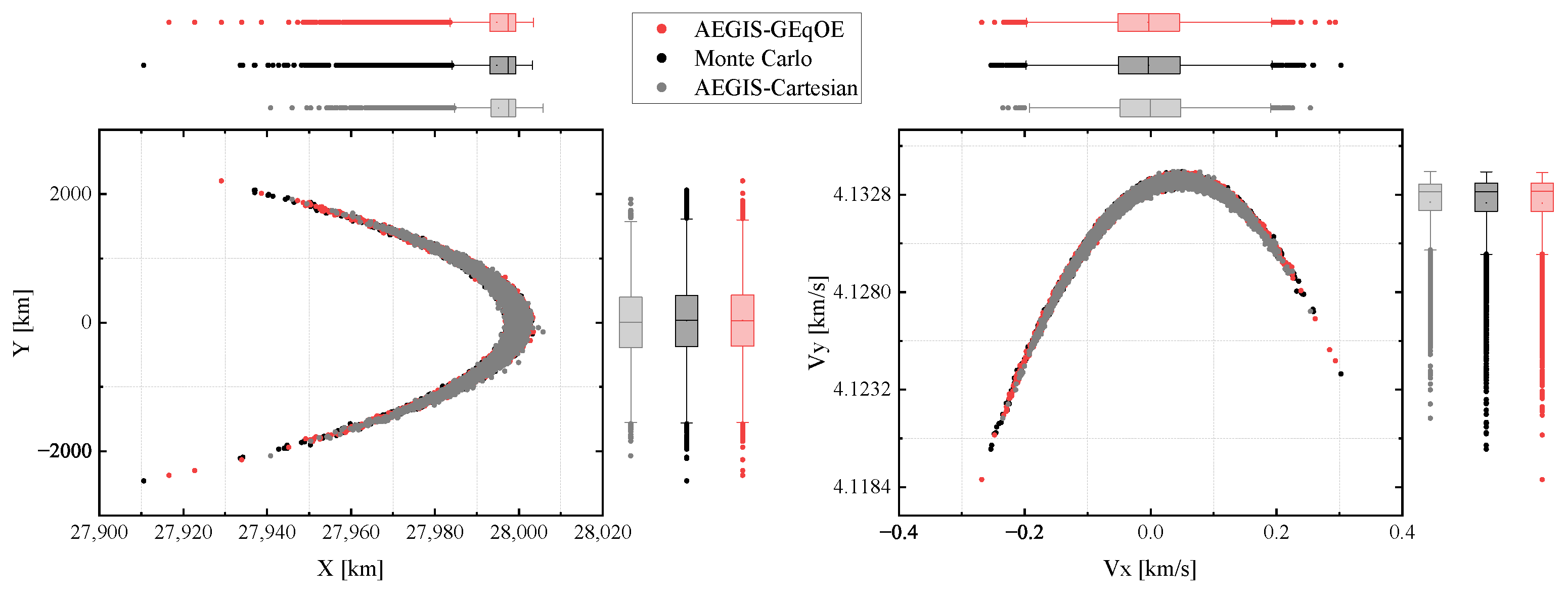
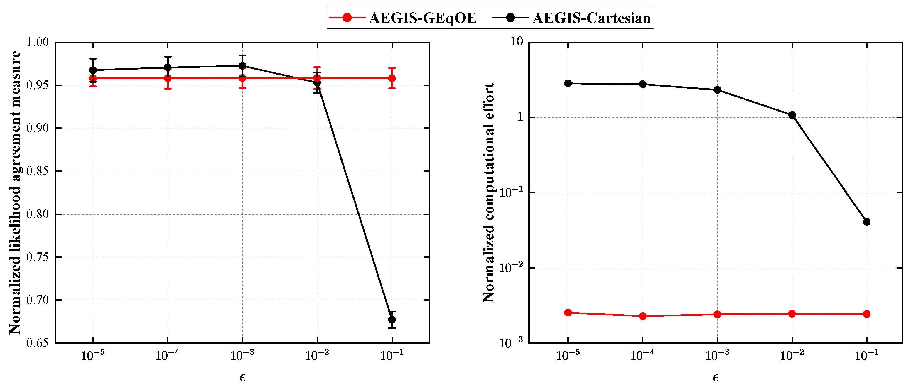
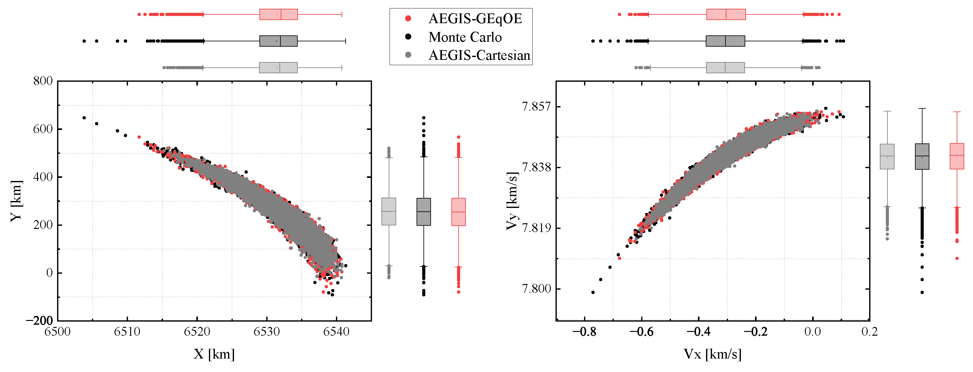
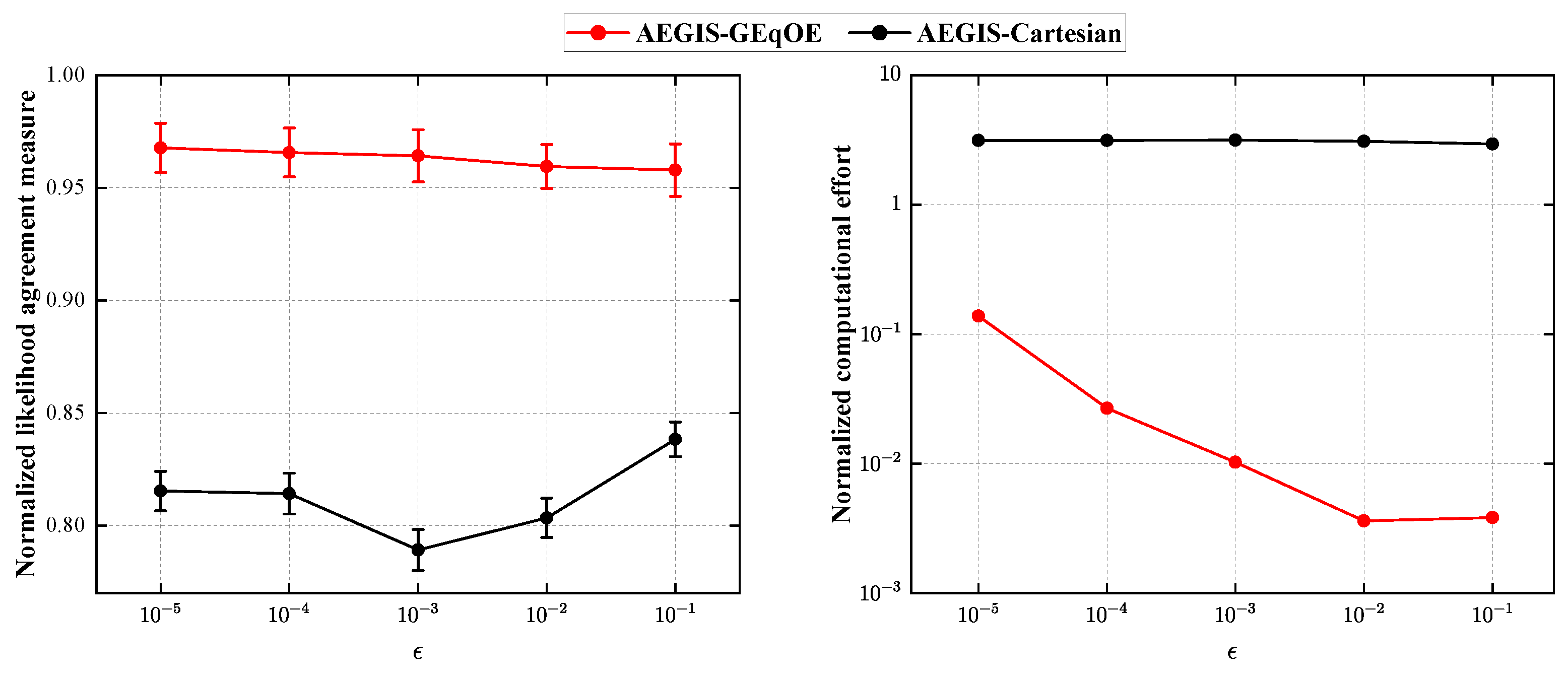
• To validate the performance of AEGIS-GEqOE in uncertainty propagation, we conduct simulation tests using three dynamics with increasing complexity. The proposed approach is compared with an adaptive GMM-UT method based on Cartesian representation. The test results show that our method achieves accuracy comparable to the MC results, while significantly reducing the number of Gaussian components compared to the Cartesian GMM approach. This demonstrates the balance achieved by our method between propagation accuracy and efficiency.

The remainder of this paper is organized as follows. Section 2 defines the uncertainty propagation problem in orbital dynamics. Section 3 provides an explanation of the motivation behind this work and presents the implementation details of the proposed adaptive GMM based on GEqOE representation. Specifically, Section 3.2 introduces two core modules: differential entropy-based GMM splitting and multidirectional GMM splitting. The formulation deduction of the GEqOE is then presented in Section 3.3. In Section 4, a performance comparison between the adaptive GMM in Cartesian and GEqOE space is conducted under three simulated scenarios: two-body, J2-perturbed, and full dynamics. A detailed discussion of the simulation test results is provided in Section 5. Finally, Section 6 concludes the paper.

2. Problem Statement

Given a nonlinear dynamical system that follows the subsequent ordinary differential equations (ODEs)

$$\dot{\mathit{x}}=\mathit{f}(\mathit{x}\left(t\right),t),\mathit{x}\left(t_0\right)={\mathit{x}}_0$$

(1)

where $\mathit{x}\left(t\right)\in {\mathbb{R}}^n$ is the state vector at time t and its initial state is ${\mathit{x}}_0$, $\mathit{f}:{\mathbb{R}}^n\to {\mathbb{R}}^n$ is a differentiable function.

When the system state has an initial error distribution $p({\mathit{x}}_0,t_0)$, the problem of uncertainty propagation arises in describing the evolution of state error over time, $p(\mathit{x},t)$. In orbital dynamics, the initial orbital uncertainty $p({\mathit{x}}_0,t_0)$ is typically defined as a Gaussian probability density function [7], fully characterized by its first-order and second-order moments (mean and variance):

$$p_g(\mathit{x};\mathit{m},\mathit{P})=\frac{1}{\sqrt{{\left(2\mathsf{\pi }\right)}^{n}det\left(\mathit{P}\right)}}\exp (-\frac{1}{2}{(\mathit{x}-\mathit{m})}^{\mathrm{T}}{\mathit{P}}^{-1}(\mathit{x}-\mathit{m}))$$

(2)

where $\mathit{m}\in {\mathbb{R}}^n$ is the reference trajectory, $\mathit{P}\in {\mathbb{R}}^{n\times n}$ is the covariance matrix, $\det (·)$ represents the determinant of the square matrix, and $\exp (·)$ is the exponential function.

Under a nonlinear map, the initial Gaussian distribution will inevitably deform into a non-Gaussian distribution after long propagation if no actions are taken. Consequently, uncertainty propagation methods that rely on the Gaussian assumption would fail. To address this issue, the Gaussian mixture model was proposed, offering a solution for describing the true PDF under Gaussian deformation. The GMM possesses the theoretical capability to accurately fit any distribution with a sufficient number of components, enabling an accurate description of the true PDF. Moreover, by dividing the deviation domain of the original distribution into multiple GMM components with smaller deviations, the nonlinear propagation of these smaller components can be locally approximated as linear propagation, thereby extending the Gaussian validity. The formulation of the GMM is obtained via

$$p\left(\mathit{x}\right)=\sum _{i=1}^L{\alpha }_i{p}_g(\mathit{x};{\mathit{m}}_i,{\mathit{P}}_i)$$

(3)

where L is the number of components and ${\alpha }_i$, ${\mathit{m}}_i$, and ${\mathit{P}}_i$ represent the associated weight, mean, and covariance of each component, respectively. To ensure the PDF is positive and the integral is 1, ${\alpha }_i$ satisfies the condition

$$\left\{\begin{array}{c}{\alpha }_i\ge 0\forall i\in \{1,2,...,L\}\\ \sum _{i=1}^L{\alpha }_i=1\end{array}\right.$$

(4)

With the assurance of approximately linear propagation over neighboring times offered by the GMM [38], some well-established propagation techniques can reliably map the means and covariances of the GMM to construct the final PDF. Mainstream works consist of two categories. The first [21,39] involves dividing the initial distribution into a sufficiently large number of components so that the deviation of each evolved component remains small enough for the linear approximation to be valid over the entire propagation period. However, determining the number of required components can be difficult, and the computation burden of propagating numerous components from the beginning to the end can be challenging. The second category [40,41] starts with a small number of components but achieves uncertainty realism by adaptively adjusting the number of components. In this paper, we investigate the second strategy, focusing on how to combine the adaptive GMM and the GEqOE representation to keep the uncertainty realism. The functional modules and specific details will be introduced in the next section.

3. Methodology

3.1. Proposed AEGIS-GEqOE

To achieve a balance of propagation accuracy and efficiency in orbital nonlinear propagation problems, we propose a novel method that combines the adaptive Gaussian mixture model with the GEqOE representation. The overall procedure of this method is depicted in Figure 1, comprising two core components: the adaptive GMM and the GEqOE propagator.

The original motivation behind incorporating GMMs into uncertainty propagation was to remove the assumption of the Gaussian distribution in state estimation while applying the extended Kalman filter to nonlinear systems [20]. The adaptive GMM (AGMM) involves two essential procedures [21,38]: nonlinear detection, which accurately identifies the breakout point of the dynamics’ uncertainty realism, and the splitting operation, which divides the detected component into multiple smaller portions. As shown in the gray functionality block of Figure 1, these two functional modules are iterated during propagation. Once the nonlinear metrics of GMM components surpass the preset threshold, the corresponding component is divided into multiple subdomains.

Specifically, under the influence of the nonlinear system, the initial Gaussian distribution of orbital uncertainty will deform. The degree of nonlinearity determines the rate at which the Gaussian distribution deforms: the more severe the nonlinearity, the faster the deformation occurs. In the traditional Cartesian dynamical system, the Gaussian validity will eventually be lost depending on the initial deviation and the length of propagation time. The required number of components of traditional AGMM to accurately describe the true PDF will increase exponentially, as a result of an increasing number of triggered splitting operations. Given the capability of orbital elements to mitigate the nonlinearity of dynamics, a natural question arises: is there a possibility of reducing the number of components in GMM-based approaches by carefully selecting orbital elements and associated dynamics? If the underlying dynamics exhibits less nonlinearity compared to Cartesian dynamics, the speed of distribution deformation slows down, delaying the occurrence of the first splitting event and increasing the interval between subsequent splittings. These effects would contribute to a reduction in the number of components.

In this paper, we have improved adaptive entropy-based Gaussian mixture information synthesis (AEGIS) by incorporating GEqOE. For the sake of brevity, we will refer to the proposed method as AEGIS-GEqOE hereafter. We first implemented a new propagator based on the GEqOE state representation. As illustrated in Figure 1, the initial Gaussian distribution is firstly transformed from Cartesian coordinates ($\mathit{x}$) to GEqOE coordinates ($\mathit{y}$). Subsequently, both the samples and PDF moment features are propagated using the GEqOE propagator. Two splitting strategies are then reformulated to accommodate the change in orbital state representation. With the reduction in nonlinearity achieved by the GEqOE, the trigger times for the splitting event can be significantly decreased, resulting in fewer components that need to be propagated in the AGMM. At the final propagation epoch, we can reconstruct the Cartesian PDF based on the GEqOE results. This entire process is equivalent to uncertainty propagation in Cartesian space, providing reliable accuracy while imposing a lower computational burden.

3.2. GMM Splitting Strategies

Different from dividing the initial uncertainty and then propagating GMM components individually as in a particle filter, the adaptive GMM starts from the original Gaussian assumption and dynamically adjusts the number of components using a well-designed splitting strategy. The goal is to trigger the splitting operation as soon as the Gaussian components can no longer adequately represent the true state PDF, typically implemented through nonlinear detectors. To achieve this, the procedure first constructs a univariate splitting library and subsequently splits the multivariate Gaussian into multiple components along a specific split direction. As a result, the multivariate Gaussian distribution transforms into the weighted sum of univariate Gaussian distributions. The distorted components are thereby replaced by smaller ones, effectively mitigating the effects of underlying nonlinearities.

3.2.1. Differential Entropy-Based Splitting

An important advancement in the adaptive GMM is due to DeMars et al. [40], who proposed using the differential entropy of covariance as the nonlinearity measure for the evolving dynamics. The differential entropy quantifies the average amount of information content associated with a random variable. For a Gaussian distribution $N(\mathit{x};\mathit{\mu },\mathit{P})$, its differential entropy can be calculated as follows:

$$H\left(\mathit{x}\right)=\frac{1}{2}log\left|2\mathsf{\pi }\mathrm{e}\mathit{P}\right|$$

(5)

where H represents the differential entropy corresponding to the Gaussian distribution, $\mathit{x}$ is the system state, $\mathrm{e}$ is the natural logarithm, and $\mathit{P}$ is the covariance matrix. In the case of a linearized dynamical system, the temporal derivative of the differential entropy can be expressed by

$$\dot{H}\left(\mathit{x}\right)=\mathrm{trace}(\mathit{F}\left(\mathit{\mu }\right(t),t))$$

(6)

where $\mathit{F}\left(\mathit{\mu }\right(t),t)$ is the Jacobian matrix of the time derivatives of the state as a function of the distribution mean $\mathit{\mu }\left(t\right)$.

In this paper, we employ the nonlinearity index introduced in [40] to identify the breakdown point of the dynamics’ uncertainty realism. This index is constructed by measuring the difference between the differential entropy of linear and nonlinear propagation, denoted as $\Delta H=|H_{nonlinear}-H_{linear}|$. Two differential entropy values are propagated over time: the value of the entropy for a linearized dynamical system, $H_{linear}$, can be calculated by numerically integrating Equation (6), while a nonlinear implementation of the integration of the covariance matrix using UT [11] is considered. The propagated covariance matrix $\mathit{P}$ can be reconstructed with the transformed sigma points, resulting in a nonlinear entropy ($H_{nonlinear}$) determined via Equation (5). The deviation of the nonlinear entropy from the linear entropy $\Delta H$ quantifies the nonlinear effects impacting the GMM component. Once the $\Delta H$ reaches a predetermined threshold $ϵ$, indicating a violation of uncertainty realism ($\Delta H-|ϵ·H_{linear}|>0$), a splitting operation is triggered.

After detecting the breakdown of uncertainty realism, it is necessary to split the original distribution into multiple components. Given the Gaussian assumption used for filter prediction and uncertainty propagation, the problem of approximating a Gaussian distribution with multiple Gaussian components has been extensively investigated. A commonly employed approach is to build a nonlinear optimization problem based on the homoscedastic simplification, i.e., all of the components have the same variance. The optimization solution used in this paper is a univariate splitting library of 3 and 5 components, which can be applied to split a multivariate GMM. The procedure is outlined in Algorithm 1. The u-th GMM component ready to be split is characterized by mean ${\mathit{\mu }}_i$ and covariance matrix ${\mathit{P}}_i$. Based on the univariate splitting library consisting of L Gaussian distributions, $\{{\tilde{\alpha }}_s$, ${\tilde{\mathit{\mu }}}_s$, ${\tilde{\sigma }}_s\}$, a set of split components $\{w_s,{\mathit{\mu }}_s,{\mathit{P}}_s\}$ can be obtained, where $s\in [1,L]$ and ${\tilde{\sigma }}_s$ denotes the standard deviation of the splitting library.

Algorithm 1 DeMars’s splitting strategy

Input: GMM component: ${\alpha }_i$, ${\mathit{\mu }}_i$, ${\mathit{P}}_i$;   univariate splitting library: $\{{\tilde{\alpha }}_s$, ${\tilde{\mathit{\mu }}}_s$, ${\tilde{\sigma }}_s\}$; Output: Splitted component set: $\{w_s,{\mathit{\mu }}_s,{\mathit{P}}_s\}$;   1: Spectral decomposition: ${\mathit{P}}_i=\vee \wedge {\vee }^{\mathrm{T}}$, where $\wedge =\mathrm{diag}\{{\lambda }_1,...,{\lambda }_n\}$.   2: Choose the splitting direction corresponding to the k-th eigenvalue ${\lambda }_k$:   3: for the s-th splitting individual of splitting library do   4:    weight update: $w_s={\tilde{\alpha }}_s{\alpha }_i$.   5:    mean update: ${\mathit{\mu }}_s={\mathit{\mu }}_i+\sqrt{{\lambda }_k}{\tilde{\mathit{\mu }}}_s{\mathit{v}}_k$, where ${\mathit{v}}_k$ is the k-th eigenvector of ${\mathit{P}}_i$.   6:    covariance update: ${\mathit{P}}_s=\vee {\wedge }_s{\vee }^{\mathrm{T}}$, where ${\wedge }_s=\mathrm{diag}\{{\lambda }_1,...,{\tilde{\sigma }}_s^2{\lambda }_k,...,{\lambda }_n\}$.   7: end for

In the implementation of AGMM, the unscented transform is employed as the moment mapping method. Starting with the initial Gaussian or GMM component, we use the unscented transform to sample featured points from the underlying PDF and then concatenate them with the initial differential entropy for time propagation. Assuming a splitting duration of $[t_{s-1},t_s]$, the initial PDF is characterized by weight ${\alpha }_i$, mean ${\mathit{\mu }}_i$, and the covariance ${\mathit{P}}_i$. According to the UT scheme, $2n+1$ sigma points can preserve the first and second statistical moments of any transformed distribution, where n is the state dimension,

$$\begin{array}{cc}\hfill & \mathcal{X}\left(0\right)={\mathit{\mu }}_i\hfill \\ \hfill & \mathcal{X}\left(j\right)={\mathit{\mu }}_i+\sqrt{n+\lambda }{\mathit{S}}_j\hfill \\ \hfill & \mathcal{X}(j+n)={\mathit{\mu }}_i-\sqrt{n+\lambda }{\mathit{S}}_j\hfill \end{array}$$

(7)

where $j\in [1,n]$, ${\mathit{S}}_j$ represents the j-th column of the Cholesky decomposition matrix $\mathit{S}$, ${\mathit{P}}_i=\mathit{S}{\mathit{S}}^{\mathrm{T}}$, and $\lambda$ is a tunable parameter. The propagated mean ${\widehat{\mathit{\mu }}}_i$ and covariance ${\widehat{\mathit{P}}}_i$ can be reconstructed by

$$\begin{array}{cc}\hfill & {\widehat{\mathit{\mu }}}_i=\sum _{j=0}^{2n}{w}_m\left(j\right)\mathcal{Y}\left(j\right)\hfill \\ \hfill & {\widehat{\mathit{P}}}_i=\sum _{j=0}^{2n}{w}_c\left(j\right)(\mathcal{Y}\left(j\right)-{\widehat{\mathit{\mu }}}_i){(\mathcal{Y}\left(j\right)-{\widehat{\mathit{\mu }}}_i)}^{\mathrm{T}}\hfill \end{array}$$

(8)

where $w_m\left(i\right)$ and $w_c\left(i\right)$ are weights and $\left\{\mathcal{Y}\right(j\left)\right\}$ represents the sigma cloud that has been propagated. During propagation, a nonlinearity threshold $ϵ$ is predefined and the $\Delta H$ is calculated in every step. If the resulting value violates the threshold $ϵ$, a splitting library with L components is applied to the propagated component along the eigenvector with the maximum eigenvalue. Finally, the original PDF of the component is approximated by the sum of splitted components:

$$\begin{array}{c}\hfill {\alpha }_i{p}_g(x;{\mathit{\mu }}_i,{\mathit{P}}_i)\approxeq \sum _{s=1}^L{w}_s{p}_g(x;{\mathit{\mu }}_s,{\mathit{P}}_s)\end{array}$$

(9)

where $p_g$ represents the Gaussian PDF.

3.2.2. Multidirectional Splitting

Considering the increasing deformation of the evolving uncertainty PDF, different degrees of nonlinearity will appear in different dimensional directions. Vittaldev et al. [4,42] propose a univariate splitting library, allowing for an arbitrary direction choice. This library supports up to $L=39$ components for a single splitting action. Additionally, multidirectional splitting can be performed in a recursive manner. If splitting along only one direction fails to capture the non-Gaussianity of the underlying distribution, each resulting component from the first splitting can be further split along the next specified direction. This procedure can be repeated multiple times, depending on the required accuracy and available computational resources. In the adaptive GMM-based approaches, we use multidirectional splitting to divide the initial distribution, aiming to decrease the splitting number during full propagation.

An arbitrary-direction splitting library is first constructed via

$$\begin{array}{cc}\hfill {\mathit{\mu }}_s& ={\mathit{\mu }}_i+\widetilde{{\mathit{\mu }}_s}\mathit{S}{\widehat{a}}^{*}\hfill \\ \hfill {\mathit{P}}_s& =\mathit{S}(\mathit{I}+({\tilde{\sigma }}_s^2-1){\widehat{\mathit{a}}}^{*}{\widehat{\mathit{a}}}^{*\mathrm{T}}){\mathit{S}}^{\mathrm{T}}\hfill \\ \hfill {\widehat{\mathit{a}}}^{*}& =\frac{{\mathit{S}}^{-1}\mathit{u}}{\left|\right|{\mathit{S}}^{-1}\mathit{u}{\left|\right|}_2}\hfill \end{array}$$

(10)

where $\{{\mathit{\mu }}_i,{\mathit{P}}_i\}$ is the moment feature of the i-th candidate component; ${\tilde{\mathit{\mu }}}_s,{\tilde{\sigma }}_s$ are the component mean and standard deviation of the splitting library, respectively; $\mathit{u}$ is the arbitrary direction vector on which the splitting operation can be performed, and $\mathit{S}$ is the square-root matrix after Cholesky decomposition for ${\mathit{P}}_i$.

The directions along which the splitting operation is performed are often chosen by a nonlinearity statistic proposed in [4],

$${\varphi }_i=\frac{f(\overline{\mathit{\mu }}+\tilde{h}{\sigma }_{\left|\right|\widehat{a}})+f(\overline{\mathit{\mu }}-\tilde{h}{\sigma }_{\left|\right|\widehat{a}})-2f\left(\overline{\mathit{\mu }}\right)}{2{\tilde{h}}^2}$$

(11)

where ${\varphi }_i$ represents the nonlinearity metric corresponding to the current splitting; $\overline{\mathit{\mu }}$ is the mean vector of the candidate component; and $\tilde{h}$ is set to $\sqrt{3}$ to align function evaluations with the sigma points along $\overline{\mathit{\mu }}$. The associated deviation along the splitting direction $\mathit{u}$ is calculated with ${\sigma }_{\left|\right|\widehat{a}}={\left|\right|{\mathit{S}}^{-1}\widehat{a}\left|\right|}_2^{-1}$.

After evaluating ${\varphi }_i$ for all candidate directions, the directions are ranked based on their nonlinearity using the 2-norm measure. By recursively choosing the interested direction to split the Gaussian distribution, the resulting components exhibit smaller deviations than the original Gaussian. While adopting the strategy described in [4] as an adaptive scheme of GMM components may lead to an unbounded growth in the number of components due to the increasing uncertainty and extending propagation time, the multidirectional splitting approach shows great potential in scenarios with highly deformed and elongated density distributions, especially in long-term uncertainty propagation. In this paper, we investigated the effectiveness of the multidirectional splitting strategy to improve the capability of the proposed AEGIS-GEqOE in dealing with highly nonlinear scenarios.

3.3. Generalized Equinoctial Orbital Elements

Recent works [34,35,36] have explored the effectiveness of the state representation for uncertainty propagation. In particular, Baù et al. [36] proposed a new set of variables to represent the orbital state that can improve propagation performance when some or all of the perturbing forces come from potential energy. The new variables are called generalized equinoctial orbital elements and are given by ($\nu ,p_1,p_2,\mathcal{L},q_1,q_2$), in which $\nu$ is the generalized form of the mean motion n, ($p_1$, $p_2$) are the generalized versions of the equinoctial orbital elements (h, k), $\mathcal{L}$ is the generalized mean longitude, and ($q_1$, $q_2$) coincide with the equinoctial orbital elements (p, q). In the following section, we will provide the mathematical formulation of GEqOE based on a nonosculating ellipse firstly, and then the equations of motion under the new coordinate representation will be presented.

3.3.1. Mathematical Formulation

Following [36], consider a point P of mass m attracted by a body of mass M. Its motion in a geocentric inertial reference frame is described by the differential equation

$$\ddot{\mathit{r}}=-\frac{\mu \mathit{r}}{r^3}+\mathit{F}(\mathit{r},\dot{\mathit{r}},t)$$

(12)

where $\mathit{r}$, $\dot{\mathit{r}}$, and $\ddot{\mathit{r}}$ are the geocentric position, velocity, and acceleration of P, respectively. The quantity $\mu$ is the gravitational parameter of the Earth, r is the position magnitude, and t denotes time. The point mass is subject to the perturbing force $\mathit{F}$ that consists of one term $\mathit{P}$ that does not arise from a potential and another one that arises from the potential energy $\mathcal{U}$:

$$\mathit{F}(\mathit{r},\dot{\mathit{r}},t)=\mathit{P}(\mathit{r},\dot{\mathit{r}},t)-\nabla \mathcal{U}(\mathit{r},t).$$

(13)

The main concept behind GEqOE is that some or all of the perturbing forces can be derived from a potential $\mathcal{U}$. The total energy $\mathcal{E}$ is the sum of the Keplerian energy ${\mathcal{E}}_K$ and the potential energy:

$$\mathcal{E}={\mathcal{E}}_K+\mathcal{U}$$

(14)

In the following, by embedding the potential energy $\mathcal{U}$ in the definition of the generalized version of angular moment, semimajor axis, and eccentricity, a nonosculating ellipse $\Gamma$ can be introduced.

First, the generalized angular momentum is defined as

$$c=\sqrt{h^2+2r^2\mathcal{U}},\mathit{c}=c{\mathit{e}}_h$$

(15)

where h denotes the magnitude of the angular moment, $h=|\mathit{r}\times \dot{\mathit{r}}|$, ${\mathit{e}}_h$ is one element of the orthonormal basis of the orbital reference frame ${\sum }_{or}=\{O;{\mathit{e}}_r,{\mathit{e}}_f,{\mathit{e}}_h\}$,

$${\mathit{e}}_r=\frac{\mathit{r}}{\left|\mathit{r}\right|},{\mathit{e}}_f={\mathit{e}}_h\times {\mathit{e}}_r,{\mathit{e}}_h=\frac{\mathit{r}\times \dot{\mathit{r}}}{|\mathit{r}\times \dot{\mathit{r}}|}$$

(16)

Moreover, the generalized velocity vector is introduced:

$$\mathit{\upsilon }=\dot{\mathit{r}}{\mathit{e}}_r+\frac{c}{r}{\mathit{e}}_f$$

(17)

Now, based on the pair of vectors ($\mathit{r}$, $\mathit{\upsilon }$), a nonosculating ellipse $\Gamma$ is defined, taking the primary body as center and lying on the orbital plane. Next, we need to determine the shape and orientation of the ellipse.

The generalized semimajor axis a and generalized eccentricity g are introduced as the following:

$$a=-\frac{\mu }{2\mathcal{E}},g=\frac{1}{\mu }\sqrt{{\mu }^2+2\mathcal{E}{c}^2}$$

(18)

The generalized eccentricity g is related to the osculating eccentricity e by

$$g^2=e^2+\frac{2\mathcal{U}}{{\mu }^2}[h^2+2r^2({\mathcal{E}}_K+\mathcal{U})].$$

(19)

The generalized Laplace vector is introduced to fix the orientation of $\Gamma$ on the orbital plane:

$$\mu \mathit{g}=\mathit{\upsilon }\times (\mathit{r}\times \mathit{\upsilon })-\mu {\mathit{e}}_r,$$

(20)

where $\left|\mathit{g}\right|=g$.

Finally, the instantaneous location of the target in the orbit should be determined by the generalized true anomaly $\theta$, defined as the angular separation between the vectors $\mathit{g}$ and $\mathit{r}$, formulated via

$$\begin{array}{c}\hfill \left\{\begin{array}{cc}gcos\theta =& \frac{c^2}{\mu r}-1,\\ gsin\theta =& \frac{c\dot{r}}{\mu }\end{array}\right.\end{array}$$

(21)

Similarly, the generalized eccentric anomaly G can be defined with the relations

$$\left\{\begin{array}{c}gcosG=1-\frac{r}{a},\\ gsinG=\frac{r\dot{r}}{\sqrt{\mu a}}\end{array}\right.$$

(22)

The generalized Kepler’s equation takes the form

$$\mathcal{M}=G-gsinG$$

(23)

where $\mathcal{M}$ is the generalized mean anomaly.

Consider the classical equinoctial reference frame ${\sum }_{eq}=\{O;{\mathit{e}}_X,{\mathit{e}}_Y,{\mathit{e}}_Z\}$. The angular displacement between the direction of ${\mathit{e}}_r$ and that of ${\mathit{e}}_X$ is called true longitude and is given by

$$L=\omega +\Omega +f$$

(24)

where $\omega$ represents the classical argument of the pericenter, $\Omega$ is the right ascension of the ascending node, and f is the true anomaly.

We are ready to introduce the generalized equinoctial orbital elements. The first three elements are defined as

$$\begin{array}{cc}\hfill \nu & \hfill :=\frac{1}{\mu }{(-2\mathcal{E})}^{3/2},\hfill \end{array}$$

(25)

$$\begin{array}{cc}\hfill p_1& \hfill :=gsin\Psi ,\hfill \end{array}$$

(26)

$$\begin{array}{cc}\hfill p_2& \hfill :=gcos\Psi ,\hfill \end{array}$$

(27)

where $\nu$ is the generalized form of the mean motion n, and $p_1$ and $p_2$ are the generalized versions of the equinoctial orbital elements h and k, defined as the projection of $\mathit{g}$ along the in-plane axes of ${\Sigma }_{eq}$. The angular variable $\Psi$, named the generalized longitude of the pericenter, is defined as

$$\Psi =L-\theta .$$

(28)

Then, the fourth element of GEqOE, the generalized mean longitude $\mathcal{L}:=\mathcal{M}+\Psi$, is introduced to fix the position of P with respect to ${\Sigma }_{eq}$. Lastly, the elements $q_1$, $q_2$ are defined as the elements p, q (see [33]), that is:

$$\begin{array}{cc}\hfill q_1& \hfill :=tan\frac{i}{2}sin\Omega ,\hfill \end{array}$$

(29)

$$\begin{array}{cc}\hfill q_2& \hfill :=tan\frac{i}{2}cos\Omega \hfill \end{array}$$

(30)

where i is the classical inclination.

The improvement in nonlinearity reduction can be attributed to the reduction in the number of fast variables used to describe the target’s location from six in Cartesian space to one in the GEqOE representation. Additionally, from the derivation process of GEqOE, it can be seen that the perturbation derived from a potential is effectively absorbed by the proposed elements. In [37], a mathematical analysis is provided to demonstrate the GEqOE’s ability to mitigate the nonlinearity effect. The closed analytical formulations, which encompass the transformations between Cartesian coordinates and the GEqOE representation, as well as the analytical expressions for the variational equations, are detailed in [36,37]. It is worth noting that the computation of the Jacobian matrix F (see Equation (6)) is essential for the time propagation of the differential entropy. All the research and efforts related to the GEqOE significantly contribute to its application in this paper, where it is employed to address the uncertainty propagation problem.

3.3.2. Time Derivatives of the GEqOE

Given the initial position ${\mathit{r}}_0$ and velocity ${\mathit{v}}_0$ at epoch time $t_0$ in an ECI frame ∑, we can obtain its GEqOE initial conditions based on the conversion equations in [36]. The state vector expressed in the GEqOE, denoted by $\mathit{y}=(\nu ,p_1,p_2,\mathcal{L},q_1,q_2)$, obeys the equation of motion:

$$\dot{\mathit{y}}=f(\mathit{y},t)$$

(31)

The Jacobian matrix $\partial f(\mathit{y},t)/\partial \mathit{y}$ can be computed analytically for GEqOE. Its derivation is not shown here for simplicity, which can be referred to in the original paper [37]. The time derivatives of the GEqOE are given by

$$\begin{array}{cc}\hfill \dot{\nu }& =-3{\left(\frac{\nu }{{\mu }^2}\right)}^{1/3}\dot{\mathcal{E}},\hfill \\ \hfill {\dot{p}}_1& =p_2\left(\frac{h-c}{r^2}-w_h\right)+\frac{1}{c}\left(\frac{X}{\mathrm{a}}+2p_2\right)(2\mathcal{U}-r{F}_r)\hfill \\ \hfill & +\frac{1}{c^2}(Y(r+\varrho )+r^2{p}_1)\dot{\mathcal{E}},\hfill \\ \hfill {\dot{p}}_2& =p_1\left(w_h-\frac{h-c}{r^2}\right)+\frac{1}{c}\left(\frac{Y}{\mathrm{a}}+2p_1\right)(2\mathcal{U}-r{F}_r)\hfill \\ \hfill & +\frac{1}{c^2}(X(r+\varrho )+r^2{p}_2)\dot{\mathcal{E}}\hfill \\ \hfill \dot{\mathcal{L}}& =\nu +\frac{h-c}{r^2}-w_h+\left(\frac{r\dot{r}\alpha }{\mu c}(r+\varrho )\right)\dot{\mathcal{E}}\hfill \\ \hfill & +\frac{1}{c}\left[\frac{1}{\alpha }+\alpha \left(1-\frac{r}{\mathrm{a}}\right)\right](2\mathcal{U}-r{F}_r),\hfill \\ \hfill {\dot{q}}_1& =\frac{1}{2}{w}_Y(1+q_1^2+q_2^2),\hfill \\ \hfill {\dot{q}}_2& =\frac{1}{2}{w}_X(1+q_1^2+q_2^2),\hfill \end{array}$$

where the time derivative of energy can be calculated via

$$\dot{\mathcal{E}}={\mathcal{U}}_t+\dot{r}{P}_r+\frac{h}{r}{P}_f$$

(32)

Here, $P_r=\mathit{P}·{\mathit{e}}_r$, $P_f=\mathit{P}·{\mathit{e}}_f$, and ${\mathcal{U}}_t$ is the partial derivative of $\mathcal{U}(\mathit{r},t)$ with respect to t. In addition, X, Y represent the target’s coordinates in the equinoctial reference frame ${\sum }_{eq}$; $w_X,w_Y,w_h$ are the projections of the angular velocity of ${\sum }_{eq}$ with respect to ∑ on the equinoctial axes; $\alpha$, $\varrho$ are the auxiliary terms. The expressions of these quantities are

$$X=rcosL,Y=rsinL$$

(33)

$$\begin{array}{c}\hfill w_X=F_h\frac{r}{h}cosL,\\ \hfill w_Y=F_h\frac{r}{h}sinL,\\ \hfill w_h=-\frac{r}{h}{F}_{h}tan\frac{i}{2}sin(w+f)\end{array}$$

(34)

where $F_h=\mathit{F}·{\mathit{e}}_h$ and

$$\alpha =\frac{1}{1+\sqrt{1-p_1^2-p_2^2}},\varrho =\frac{c^2}{\mu }$$

(35)

4. Results

In this section, we implement a series of simulation tests to validate the performance of the proposed AEGIS-GEqOE method. First, in Section 4.1, we perform a Cramer–von Mises test on a classical LEO case to verify the extension of Gaussianity achieved by the GEqOE representation for uncertainty propagation. Then, in Section 4.2, we simulate three dynamics scenarios with increasing complexity and compare the proposed AEGIS-GEqOE with the Cartesian GMM-based method and the Monte Carlo method to assess its ability to balance propagation accuracy and efficiency.

For all simulation tests, the initial epoch time is set to 1 January 2020 00:00:00 UTC. The state propagation under various dynamics representations can be implemented using MATLAB’s ode113 (a variable-order Adams–Bashforth–Moulton PECE solver [43]) based on the corresponding equations of motion. The relative and absolute tolerance of the propagator is set to ${10}^{-10}$.

4.1. Uncertainty Realism Evolution

By employing an appropriate state representation in uncertainty propagation, the nonlinearity of the dynamics can be mitigated, thereby extending the time period before the uncertainty realism achieved by the Gaussian distribution starts to breaks down. In this subsection, we evaluate the ability of various state representations in preserving Gaussianity during uncertainty propagation, providing essential support for the state representation choice of the proposed UP method.

The following test employs five sets of orbital elements for uncertainty propagation. We first use a formulation based on the Cartesian coordinates due to its wide application in space surveillance, and the classical GMM-based UP method, implemented in Section 4.2, is also formulated based on it. The second formulation is given by the equinoctial orbital elements (EqOE), which is one of the most commonly used nonsingular element sets for mitigating the nonlinear effect from $1/r^2$. The alternate set of elements (AEqOE), a representation that replaces the semimajor axis of EqOE with the mean motion, is used for performance comparison against the recent GEqOE, considering its important advance in this research field. Lastly, we include in the comparison with the J2EqOE [35] a set of orbital elements devised for reducing the nonlinearity arising from the J2 term of the geopotential. To demonstrate the superior ability of GEqOE in extending Gaussian validity, we choose a J2-perturbed LEO test case from [35], and the mean and variance of each of the orbital elements are shown in

Table 1. Initial state moment in LEO for Cramer–von Mises test (angles are in degrees).

a, km	e	i	$\Omega$	$\omega$	M
7136.6	0.00949	72.9	116	57.7	105.5
${\sigma }_a$, km	${\sigma }_{p_1}$	${\sigma }_{p_2}$	${\sigma }_{q_1}$	${\sigma }_{q_2}$	${\sigma }_l$
20	${10}^{-3}$	${10}^{-3}$	${10}^{-3}$	${10}^{-3}$	${10}^{-2}$

. The propagation duration is set to 1 day to ensure that the uncertainty realism under different coordinate choices is distinguishable at the final epoch.

4.1.1. Cramer–Von Mises Test

The Cramer–von Mises (CvM) test, as used in [35], is employed to assess the performance of different coordinate choices in UP. The Mahalanobis distance measures the deviation of a sample from its distribution. The squared Mahalanobis distance is defined as

$${\mathcal{M}}^{\left(i\right)}({\mathit{x}}^{\left(i\right)};\mathit{\mu },\mathit{P})={({\mathit{x}}^{\left(i\right)}-\mathit{\mu })}^{\mathrm{T}}{\mathit{P}}^{-1}({\mathit{x}}^{\left(i\right)}-\mathit{\mu }),$$

(36)

where ${\mathit{x}}^{\left(i\right)}$ is the state sample, $\mathit{\mu }$ denotes the state mean, and $\mathit{P}$ is the covariance matrix. In the orbital uncertainty propagation, if the true distribution is Gaussian, then the variable ${\mathcal{M}}^{\left(i\right)}$ will exhibit a chi-squared distribution (${\chi }^2$) with six degrees of freedom. Its cumulative distribution function (CDF) can be calculated as follows:

$$F\left(z\right)=1-\frac{1}{8}\exp (-\frac{z}{2})(z^2+4z+8)$$

(37)

where z represents the squared Mahalanobis distance.

Two propagation procedures will be performed during the CvM test. The first involves propagating the feature moment under the selected representation. The second procedure propagates Monte Carlo samples from the initial distribution in Cartesian coordinates. At the final epoch, the MC samples are converted into the target’s representation. Then, the discrepancy between the empirical distribution function statistic and the expected ${\chi }^2$ provides a quadratic term to qualify the uncertainty realism under the target representation:

$$Q=\frac{1}{12k}+\sum _{i=1}^k{[\frac{2i-1}{2k}-F\left(z^{\left(i\right)}\right)]}^2$$

(38)

where k is the total amount of samples sorted in increasing order by Mahalanobis distance.

4.1.2. Changes of Uncertainty Realism under Different State Representations

When evaluating the effect of different representations, the null hypothesis of the CvM test is that the candidate distribution is subject to the ${\chi }^2$ distribution. A threshold of the CvM test statistic to ensure uncertainty realism is set to 1.16, corresponding to a 99.9% confidence level. In this test, a total of k = 10,000 samples of the initial orbital uncertainty are propagated within the dynamics.

The CvM test statistic for a LEO scenario [35] is depicted in Figure 2, which was obtained by propagating the PDF of different state representations through the UT. For the PDF to be realistic (with 99.9% confidence), the metric value should fall within the shaded region. Observing Figure 2, it becomes evident that the uncertainty realism remains consistent under the Cartesian representation for the shortest duration, as the CvM test value exceeds the threshold line of 1.16 shortly after propagation begins (approximately within 0.028 orbital periods). Conversely, the statistical values of EqOE, AEqOE, and J2EqOE surpass the threshold line for 3.925, 3.665, and 12.149 orbital periods, respectively. Remarkably, the GEqOE maintains uncertainty realism throughout the entire one-day propagation, indicating its superiority over other representations.

4.2. Numerical Simulations

In this section, different uncertainty propagation methods are compared with the Monte Carlo results in three scenarios to evaluate their accuracy and efficiency. These scenarios involve various dynamics, including pure two-body dynamics for a high Earth orbit (HEO), J2-induced dynamics for a low Earth orbit (LEO), and full dynamics with an $8\times 8$ gravity model and lunisolar perturbations for a medium Earth orbit (MEO). These scenarios present force models of increasing complexity that allow evaluating the applicability of the proposed GEqOE-AEGIS to preserve uncertainty realism under different perturbations. The HEO and LEO cases are adapted from [40], while the MEO scenario is a circular, inclined orbit of the Galileo constellation, as used in [10] to highlight the great reduction in the number of kernels achieved through Taylor polynomials.

• Dynamic modeling

We consider here the gravitational perturbations arising from the nonspherical shape of the Earth and the third-body gravitational attraction of the Moon and the Sun. The acceleration ${\mathit{a}}_{grav}$ from the Earth’s gravity potential $\mathrm{U}$ is equal to the gradient of $\mathrm{U}$, as shown below:

$$\begin{array}{cc}\hfill & \mathrm{U}=\frac{GM}{r}\sum _{n=0}^{\infty }\sum _{m=0}^n\frac{R^n}{r^n}{P}_{nm}(sin\varphi )(C_{nm}cos\left(m\lambda \right)+S_{nm}sin\left(m\lambda \right))\hfill \\ \hfill & {\mathit{a}}_{grav}=\nabla \mathrm{U}\hfill \end{array}$$

(39)

where $GM$ denotes the gravitational parameter of the Earth, while R and r represent the Earth’s radius and the magnitude of the target’s position vector, respectively. $P_{nm}$ is the Legendre polynomial of degree n and order m; $C_{nm}$ and $S_{nm}$ are the geopotential coefficients, which correspond to different gravity models. In this paper, we have adopted the Grace gravity model 03 GGM03C [44]. Additionally, $\lambda$ and $\varphi$ denote the geocentric longitude and latitude, respectively.

The third-body gravitational acceleration ${\mathit{a}}_{3bd}$ is expressed by

$${\mathit{a}}_{3bd}=GM(\frac{\mathit{s}-\mathit{r}}{{\left|\mathit{s}-\mathit{r}\right|}^3}-\frac{\mathit{s}}{{\left|\mathit{s}\right|}^3})$$

(40)

where $\mathit{r}$ and $\mathit{s}$ are the geocentric coordinates of the target and of the celestial body. The positions of celestial bodies are obtained from the JPL DE440 ephemeris [45].

It should be noted that, as shown in Equation (13), the perturbed force comprises a term that is derivable from the potential energy $\mathcal{U}$ and a term $\mathit{P}$ that is not. In the GEqOE representation, all terms in the potential of the used gravity model (except for the point mass potential) are included in the potential energy.

With the dynamic model in place, we can formulate the time rate of the differential entropy of the linearized dynamics as follows (see Equation (6)):

$$\begin{array}{cc}\hfill \dot{H}\left(\mathit{x}\right)& =\mathrm{trace}\left\{F\right(\mathit{m}\left(t\right),t\left)\right\}\hfill \\ \hfill & =\sum _{i=1}^n\frac{\partial f_i(\mathit{x}\left(t\right),t)}{\partial x_i\left(t\right)}\hfill \end{array}$$

(41)

where $\mathit{x}$ can be the state expressed in the Cartesian or GEqOE space and F represents the Jacobian matrix of the underlying dynamics.

• Scenario setup

The initial orbital uncertainties are assumed Gaussian in the following simulated scenarios, and their initial reference orbital elements are summarized in

Table 2. Initial orbital elements for three scenarios (angles are in degrees).

Case	a, km	e	i	$\mathbf{\Omega }$	$\mathbf{\omega }$	M
LEO	6603.0	0.01	0.0	0.0	0.0	0.0
HEO	35,000.0	0.2	0.0	0.0	0.0	0.0
MEO	29,600.135	0.0	56.0	0.0	0.0	0.0

, followed by

Table 3. The standard deviation values of the Cartesian states for three scenarios.

Case	x, km	y, km	z, km	${\mathit{v}}_{\mathit{x}}$, km/s	${\mathit{v}}_{\mathit{y}}$, km/s	${\mathit{v}}_{\mathit{z}}$, km/s
LEO	1.3	0.5	1.0	$2.5\times {10}^{-3}$	$5.0\times {10}^{-3}$	$0.5\times {10}^{-3}$
HEO	1.0	1.0	1.0	$1.0\times {10}^{-3}$	$1.0\times {10}^{-3}$	$1.0\times {10}^{-3}$
MEO	0.5	1.0	1.0	$0.5\times {10}^{-3/2}$	$0.5\times {10}^{-3/2}$	$0.5\times {10}^{-3/2}$

where the $1\sigma$ deviations of the Cartesian states for each scenario are given. The setting of the orbital elements is properly adjusted on the basis of [10,40], to build a dynamic simulation with a different perturbation complexity.

In the following, we conduct a comparison of adaptive GMM methods based on different element representations, namely AEGIS-Cartesian and AEGIS-GEqOE, in three dynamical models. The results of Monte Carlo simulations are used to evaluate the performance of different approaches. The performance metric utilizes the likelihood agreement measure, as described in [40]. Additionally, we investigate the impact of multidirectional splitting for initial uncertainty on the proposed AEGIS-GEqOE in the high-nonlinearity MEO scenario.

4.2.1. Definition of the Accuracy Measure

To assess the representation accuracy of different propagation methods compared to MC, the classical likelihood agreement measure (LAM) between two distributions is adopted as the evaluation criterion:

$$\mathcal{L}(p,q)=\frac{1}{K}\sum _{i=1}^K(\sum _{j=1}^L{\alpha }_j{p}_g({\mathit{\mu }}_i;{\mathit{m}}_j,{\mathit{P}}_j))$$

(42)

where K is the MC sampling number, set to 10,000 in the following tests; L is the number of Gaussian components; ${\mathit{\mu }}_i$ is the center of the Dirac delta distribution, equal to the i-th MC sample; and ${\alpha }_j$, ${\mathit{m}}_j$, and ${\mathit{P}}_j$ are the weight, mean, and covariance matrix of the Gaussian components, respectively.

The LAM value describes the amount of overlap between two PDFs. Since the distribution PDFs obtained by UP approaches are represented in different coordinate systems, in order to ensure a fair performance evaluation, we fit the Monte Carlo samples, generated through Cartesian nonlinear dynamics, with a GMM comprising 100 components. Then, we sample from the propagated PDFs in different coordinate spaces and transform them into the Cartesian space. This enables us to perform LAM calculations using the fitted GMM and the transformed samples. A higher LAM value indicates a more accurate description of the propagated PDF. In the subsequent performance presentation, we aim to provide an intuitive comparison of different methods’ performance. Therefore, we normalize the LAM based on the highest value among the test results. Similarly, the computational effort, defined as the consumed time of UP methods, will be also normalized based on the MC effort.

4.2.2. HEO Two-Body Dynamics

The results obtained by applying AEGIS-Cartesian and AEGIS-GEqOE in the two-body HEO test case are presented in this section. The initial Gaussian PDF is converted from the given Keplerian orbital elements and associated Cartesian covariance to the respective Cartesian and GEqOE representations using the unscented transform. Previous research [35] has shown that the resulting Gaussian PDF in the transformed representation can be regarded as “truth” for the purpose of initiating the Monte Carlo samples. During the adaptive splitting process, a fixed threshold is utilized for detecting nonlinearity. If the deviation of differential entropy $\Delta H$ exceeds this threshold, a splitting strategy will divide the corresponding component into three subcomponents. To prevent an exponential increase in the number of components during uncertainty propagation, a minimum weight value is set to avoid excessive computation consumption. Components with a weight less than 0.001 will not be split and will be propagated until the final epoch.

The performance of adaptive GMM-based approaches is greatly influenced by the splitting threshold, $ϵ$. Therefore, it is crucial to test the scores of both approaches (Cartesian and GEqOE) for different $ϵ$ values and choose the best for the purpose of comparison. In this simulation, K = 10,000 Monte Carlo samples are randomly generated from the initial Gaussian distribution and are propagated through nonlinear orbital dynamics. Two competing algorithms for uncertainty propagation are employed, each following its respective set of equations of motion. Given different values of $ϵ=\{{10}^{-5},{10}^{-4},{10}^{-3},{10}^{-2},{10}^{-1}\}$, the LAM and computational effort are recorded and normalized. Specifically, the LAM values obtained from all runs are divided by the maximum LAM value, and the computation efforts are normalized by Monte Carlo running times.

Figure 3 illustrates that the LAM curve of AEGIS-GEqOE exhibits less fluctuation, and the best score in the HEO scenario is achieved by AEGIS-GEqOE when $ϵ=0.1$. Furthermore, the results of normalized computational effort indicate that AEGIS-GEqOE achieves significant efficiency gains across all values of $ϵ$. This consistency is attributed to the absence of any splitting events during the propagation of AEGIS-GEqOE, which is also supported by the findings in Section 4.1.2. Similar to the traditional GMM-based approaches, AEGIS-Cartesian reduces the computation time compared to Monte Carlo when $ϵ$ is small, but it fails to accurately capture the true PDF. However, as the $ϵ$ decreases, AEGIS-Cartesian can achieve great accuracy improvement at the cost of increased computational effort.

Next, the propagation results for the best cases of the two methods are projected on the $x-y$ and $v_x-v_y$ planes in Cartesian space, as shown in Figure 4. The black dots on the projection plan represent the density distribution obtained through the Monte Carlo propagation. The shape of the distribution appears as a crescent in both the position and velocity planes, indicating that severe nonlinear effects were encountered during the propagation process. A comparison of the results with the Monte Carlo simulation reveals that both methods successfully capture the basic shape of the true PDF. However, the tail part of the true distributions cannot be accurately recovered with the Cartesian GMM method. This is evident from the plots of the marginal probability distribution in Figure 4. The box plot reveals several outlier points in the Monte Carlo output, which are also obtained via the GEqOE. Nevertheless, it is evident that the Cartesian GMM fails to capture these outliers effectively.

4.2.3. LEO J2-Induced Dynamics

In this section, we simulate an orbit influenced by J2 perturbations to demonstrate the capability of UP methods in handling complex perturbation scenarios. The orbiting object is placed in LEO, and its orbital Keplerian elements and associated covariance are provided in Table 2 and Table 3. The splitting threshold is set to $\{{10}^{-5},{10}^{-4},{10}^{-3},{10}^{-2},{10}^{-1}\}$, and a minimum weight constraint of 0.001 is also applied.

The behavior of the implemented approaches with respect to different values of $ϵ$ is presented in Figure 5. In this scenario, the AEGIS-GEqOE with $ϵ={10}^{-3}$ achieves the best score. As for the HEO test case, there were no splitting events during propagation. The trend lines for the likelihood deviation and computational effort of AEGIS-GEqOE show minimal change, resulting in a significant reduction in required computational effort compared to Monte Carlo of two orders of magnitude. Concerning AEGIS-Cartesian, it achieves its worst score in terms of LAM for $ϵ={10}^{-1}$, despite obtaining a $10\times$ speedup. With smaller values of $ϵ$, AEGIS-Cartesian shows competitive results similar to AEGIS-GEqOE, but it demands greater computational effort than Monte Carlo.

From the visualization of the distribution of position and velocity in the final epoch, a high deformation can be seen in both projection planes of Figure 6. In the position plane, the gray points show that the AEGIS-Cartesian PDF concentrates on the central part and exhibits a more diffuse volume compared to the Monte Carlo results. Furthermore, AEGIS-Cartesian struggles to accurately capture the tail distribution, especially in the x direction. On the other hand, AEGIS-GEqOE, represented by the red scatter, closely approximates the true PDF distribution, with only minor mean divergence in the x and $V_y$ directions. In this LEO scenario, the tails of the marginal distributions shown in Figure 6 can be properly reproduced by using GEqOE, while they are missing when using Cartesian variables.

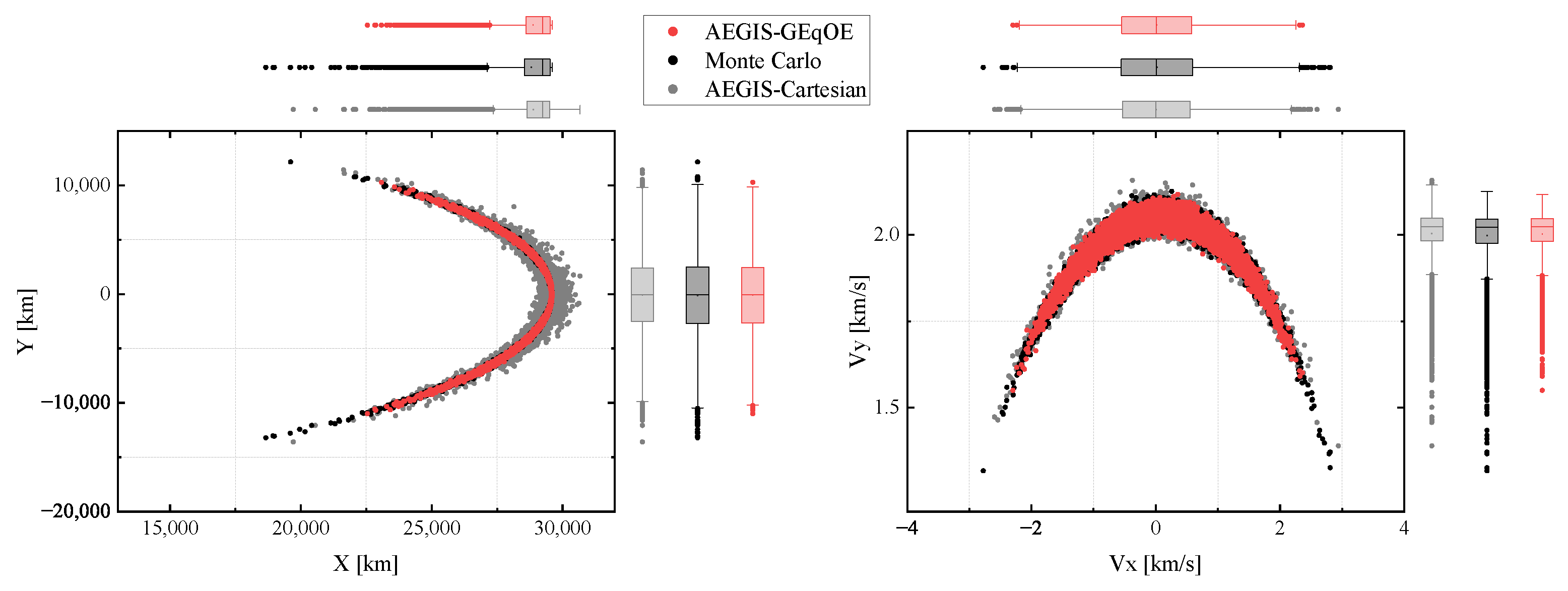
4.2.4. MEO Full Dynamics

In this section, we investigate the performance of AEGIS-GEqOE in propagating a large initial uncertainty through a more realistic dynamical model. Since no splitting event occurred in the previous test cases with AEGIS-GEqOE, we conduct a simulation on a medium Earth orbit (MEO) affected by an $8\times 8$ gravity model and lunisolar perturbation. To further ensure the occurrence of the splitting event in the AEGIS-GEqOE implementation, the initial uncertainty of the velocity is increased by a factor of two in this simulation. To handle uncertainty propagation in this highly nonlinear scenario, two AEGIS-GEqOE methods without and with multidirectional splitting are implemented for further investigation of the advancements offered by the GEqOE representation.

• Without Multidirectional Splitting

Figure 7 presents the changes in accuracy and efficiency of AEGIS-GEqOE and AEGIS-Cartesian under different $ϵ$ values. It is evident that AEGIS-GEqOE consistently achieves higher LAM scores than AEGIS-Cartesian across all $ϵ$ values, with the best LAM observed when $ϵ={10}^{-5}$. Moreover, the LAM curve of AEGIS-GEqOE exhibits an upward trend along the descending $ϵ$. A smaller $ϵ$ implies that more splitting events are triggered to increase the number of components, leading to improved accuracy at the expense of increased computation time, as evident from the normalized computational effort plot. The time consumption of AEGIS-GEqOE gradually increases, but it remains significantly lower than the computational effort required by Monte Carlo simulations and also smaller than that of AEGIS-Cartesian.

The number of propagated components using different approaches for different values of $ϵ$ is recorded in Figure 8. In the left plot, we observe a sharp increase in the number of AEGIS-Cartesian components shortly after the initial epoch. Moreover, the final number of components of AEGIS-Cartesian for all considered values of $ϵ$ reaches the upper limit allowed by the minimum weight constraint, which is 887. This indicates that AEGIS-Cartesian cannot deal with highly nonlinear dynamics effectively. On the other hand, the right plot displays a gradual change in the component number for AEGIS-GEqOE. The first splitting times in AEGIS-GEqOE implementation are $\{-,-,1.7185,1.5174,0.6146\}$ orbital periods, and the final component numbers are $\{1,1,9,27,149\}$, arranged in decreasing order of $ϵ$. The growth rate of component numbers is related to the splitting threshold. The smaller the threshold, the faster the growth of the components.

Finally, the best results obtained with the two state representations are presented in Figure 9. The scatter plots in both the position and velocity planes demonstrate that both AEGIS-Cartesian and AEGIS-GEqOE capture the basic features of the true distribution. However, the dispersion of AEGIS-Cartesian in the X extends the range of the MC distribution, resulting in a slightly divergent representation. On the other hand, AEGIS-GEqOE nearly perfectly captures the true PDF, albeit losing some outlier records at the tail of the distribution, as depicted in Figure 9. Despite this, when considering the LAM value as the performance criterion, AEGIS-GEqOE still outperforms AEGIS-Cartesian in terms of accuracy.

• With Multidirectional Splitting

Since this test case is affected by a high nonlinearity, an alternative to further advance the capability of adaptive GMM-based UP methods is combining the proposed method with multidirectional splitting at the initial epoch [41]. In this subsection, we conduct a series of tests on the AEGIS-GEqOE with $\{9,25,49\}$ initial components for performance comparison. Multidirectional splitting is performed using the univariate library proposed in [4,42] in the two directions with the maximum nonlinearity.

Specifically, AEGIS-based methods will dynamically adapt the number of propagated components based on the used splitting threshold $ϵ$. Considering the refinement of the initial uncertainty enabled by multidirectional splitting, the splitting threshold is set as $\{0.001,0.01,0.1,0.2,0.3,0.4\}$ for testing. To better evaluate the performance of different methods, the best score of AEGIS-GEqOE without multidirectional splitting achieved with $ϵ={10}^{-5}$ is chosen as the LAM basis to normalize the accuracy behavior.

The left plot of Figure 10 is the normalized LAM based on the best LAM obtained by AEGIS-GEqOE without initial splitting. It shows that a better performance is obtained by applying a nine-component splitting to the initial distribution. It can be also seen that a small threshold cannot provide accurate results when initial splitting is performed. On the other hand, the right plot depicts the normalized computational effort in units of consumed time from Monte Carlo. As the number of initial splittings increases, it becomes evident that the computational effort of the proposed method also rises. However, AEGIS-GEqOE equipped with multidirectional splitting consistently exhibits a lower computational burden than MC.

5. Discussion

This paper proposes a method that combines the GEqOE representation with the adaptive GMM for uncertainty propagation. Unlike the Cartesian coordinate representation, the proposed method utilizes the GEqOE representation to mitigate the impact of nonlinear dynamics on uncertainty realism. Consequently, the number of GMM components needed to maintain uncertainty realism is reduced, enabling significant improvements in computational efficiency while maintaining the accuracy of the propagated PDF representation. Four simulation tests are designed to evaluate the performance of the proposed method in uncertainty propagation. Firstly, the effectiveness of the GEqOE representation in absorbing nonlinearity is validated using the Cramer–von Mises test. Secondly, three application scenarios are designed to compare the accuracy and computational efficiency of two methods: AEGIS-Cartesian and AEGIS-GEqOE. In this section, the simulation results are discussed.

5.1. Uncertainty Realism Evolution with Different Representations

Unlike traditional methods that reduce the number of GMM components, the proposed method aims to establish a mathematical formulation for weakening the nonlinearity in the equations of motion through variable transformations. This approach allows for a substantial reduction in propagated components in the adaptive GMM by effectively decreasing the frequency of splitting events. Section 4.1 presents a simulation of an uncertainty propagation using UT implementation to verify the effectiveness of the GEqOE. The initial uncertainty distribution is propagated using five different coordinate representations, and the Cramer–von Mises test is conducted based on the moment features and Monte Carlo results during the propagation process.

The test results demonstrate that the orbital elements-based representation significantly extends the duration of uncertainty realism compared to the Cartesian coordinate representation, which experiences early-stage deformation during propagation. This finding is consistent with the results presented in [35]. With increasing propagation time, the representations EqOE, AEqOE, and J2EqOE gradually deviate from the true PDF description, encountering failures at propagation periods of 3.925, 3.665, and 12.149, respectively. On the other hand, the GEqOE exhibits stable statistical performance throughout the test, with the statistical quantities remaining within the reliable range indicated by the gray region even after a propagation duration of one day. This suggests that the state can still be accurately described by a Gaussian distribution in this coordinate representation.

In summary, the results of this test demonstrate that the GEqOE representation outperforms other commonly used coordinate representations in maintaining uncertainty realism. This lays the groundwork for integrating the GEqOE and adaptive GMM. However, it is important to note that the ability to maintain uncertainty realism under a fixed coordinate representation is influenced by factors such as the propagation duration, complexity of the dynamics, and initial deviation size. Relying solely on coordinate transformation strategies to accurately describe the evolution of real deviations in all scenarios may not be realistic.

5.2. Performance Analysis of the Accuracy and Computational Efficiency for the Proposed Method

To validate the performance of the adaptive GMM propagation with the GEqOE in uncertainty propagation applications, we conduct simulations of three test cases that differ in the initial orbit and the considered dynamical model. Considering the significant impact of the splitting threshold $ϵ$ on the performance of the algorithm within the adaptive Gaussian evolution framework, we statistically analyze the algorithm’s performance at different thresholds. Based on this analysis, we select the best-performing AEGIS-Cartesian and AEGIS-GEqOE in terms of accuracy, as measured by the LAM, for comparison. Additionally, we evaluate the execution efficiency of the two methods AEGIS-Cartesian and AEGIS-GEqOE by testing and comparing their time consumption for propagation with that of the Monte Carlo method. In this simulation, we consider the Monte Carlo propagation results from 10,000 trials as the mapping results of the real distribution.

In Section 4.2, the HEO, LEO, and MEO test cases present an increasing level of complexity of the perturbations included in the dynamical model. The applicability performance of the proposed method is validated in these three scenarios. Specifically, in the HEO and LEO scenarios, AEGIS-GEqOE did not trigger any splitting events and achieved the best scores during the propagation process for two periods, resulting in a speedup of over a hundred times compared to Monte Carlo propagation. Additionally, AEGIS-GEqOE outperforms AEGIS-Cartesian when measuring the accuracy of the final results using the LAM. It is worth mentioning that AEGIS-Cartesian undergoes multiple triggers for splitting events during the propagation process due to the unmitigated nonlinearity of the underlying dynamics. Its performance improves as the splitting threshold decreases, a gain brought by the increment in the number of propagated components. At a threshold of 0.1, AEGIS-Cartesian exhibits a significant difference in the LAM compared to AEGIS-GEqOE. At a threshold of 0.01, AEGIS-Cartesian achieves comparable accuracy to AEGIS-GEqOE with a higher computational cost than Monte Carlo propagation. Furthermore, as the threshold increases, the number of splitting events triggered in AEGIS-Cartesian also increases, causing the number of components to quickly reach the upper limit allowed by the minimum weight constraint. At this point, the performance of the AEGIS-Cartesian algorithm does not improve.

From the simulation results in these two scenarios, it can be seen that AEGIS-GEqOE weakens the underlying dynamics’ nonlinearity, enabling an accurate representation of the true PDF with fewer components. The position and velocity projections in Figure 4 and Figure 6 provide intuitive visualization evidence for this.

To further verify the capabilities of AEGIS-GEqOE in handling complex force scenarios, we conducted a simulation involving an MEO test case with higher-order Earth gravity field and lunisolar perturbations. The initial orbit was intentionally set with a considerable deviation in the velocity direction to ensure that AEGIS-GEqOE could trigger splitting events. In this scenario, we also test the AEGIS-GEqOE method integrated with initial multidirectional splitting to investigate the effect of this strategy combination when applied to highly nonlinear dynamics propagation.

In Figure 7, it can be observed that AEGIS-GEqOE outperforms AEGIS-Cartesian in terms of the LAM under different threshold settings, and the best performance is achieved at a threshold of ${10}^{-5}$. In terms of computational effort, due to the increased number of splitting events and the growing number of propagated components, the time consumption of AEGIS-GEqOE gradually increases as threshold decreases. On the other hand, the computational consumption of AEGIS-Cartesian does not change a lot with $ϵ$, since for all considered values of $ϵ$ the maximum number of components is reached after less than one orbital period (see Figure 8, left). This indicates that the generated components from AEGIS-Cartesian cannot well capture the true evolution of the PDF. Concerning the variation in the number of components with $ϵ$, we can see that for both approaches a smaller splitting threshold leads to an earlier occurrence of the first splitting event. The left plot of Figure 8 shows that AEGIS-Cartesian experiences an early splitting event for all values of $ϵ$ and the number of splitting components increases at a fast rate. From the right plot, it is apparent that AEGIS-GEqOE has a long interval before the first splitting. Moreover, for all the considered thresholds, the first splitting event is triggered later for AEGIS-GEqOE than for AEGIS-Cartesian, resulting in a smaller number of components at the end of propagation. During propagation, the number of components of AEGIS-GEqOE never reaches the upper limit corresponding to the minimum weight constraint, which indicates that in the presence of complex perturbations and significant initial deviations, AEGIS-GEqOE, benefiting from the absorption effect on nonlinearity, can still effectively measure the true distribution during propagation through adaptive splitting. The position and velocity projections in Figure 9 provide a visual comparison between the Monte Carlo propagation and that of AEGIS-GEqOE, further confirming the excellent performance of the proposed method in balancing propagation accuracy and execution efficiency.

In Figure 10, the performance behavior of AEGIS-GEqOE with and without multidirectional splitting in the initial distribution is presented. It can be seen that a good LAM score can be obtained with the help of initial splitting, but the time for propagation would increase. A refinement of the initial distribution would make the implemented approach have a good LAM with a loose threshold for splitting. Moreover, a suitable initial number of components should be explored to achieve a balance of accuracy and efficiency, because the performance of the UP approach is not proportional to the number of components, as can be seen from the fact that the best score is obtained by the nine-component strategy.

6. Conclusions

In this paper, we present an improved GMM-based UP method that tackles the issue of computational complexity from the perspective of orbital state representation. Unlike traditional GMM component reduction approaches, a mathematical reformulation of the underlying dynamics is deployed to maintain the accuracy of the true evolving PDF while significantly reducing the computational effort. This is achieved by replacing the Cartesian coordinates with generalized equinoctial orbital elements (GEqOE), recently introduced by Baù et al. [36], which greatly mitigate nonlinear effects during distribution propagation. As a result, our proposed method extends the validation period of uncertainty realism and reduces the number of components during uncertainty propagation. To assess the performance of the proposed method, we simulated three scenarios of increasing complexity and compared them with the Monte Carlo and Cartesian GMM-based UP methods. The performance metric and the obtained results demonstrate that the propagated PDF from AEGIS-GEqOE is consistent with the Monte Carlo results. Moreover, the proposed method exhibits superior execution efficiency compared to AEGIS-Cartesian, validating both the accuracy and efficiency of this uncertainty propagation scheme. It is worth noting that this paper focuses on exploring and analyzing the impact of the gain generated from AEGIS-GEqOE’s capability of absorbing the nonlinearity from the gravity term of the adaptive GMM method. In future work, we may consider more complex dynamics, and potential research directions may involve investigating the applicability of different splitting strategies in these more complex scenarios.

References

1. Wang, Y.; Chen, X.; Ran, D.; Zhao, Y.; Chen, Y.; Bai, Y. Spacecraft formation reconfiguration with multi-obstacle avoidance under navigation and control uncertainties using adaptive artificial potential function method. Astrodynamics 2020, 4, 41–56. [Google Scholar] [CrossRef]
2. Qiao, D.; Zhou, X.; Li, X. Analytical configuration uncertainty propagation of geocentric interferometric detection constellation. Astrodynamics 2023, 7, 271–284. [Google Scholar] [CrossRef]
3. Wittig, A.; Di Lizia, P.; Armellin, R.; Makino, K.; Bernelli-Zazzera, F.; Berz, M. Propagation of large uncertainty sets in orbital dynamics by automatic domain splitting. Celest. Mech. Dyn. Astron. 2015, 122, 239–261. [Google Scholar] [CrossRef]
4. Vittaldev, V.; Russell, R.P. Space Object Collision Probability Using Multidirectional Gaussian Mixture Models. J. Guid. Control Dyn. 2016, 39, 2163–2169. [Google Scholar] [CrossRef]
5. Bierbaum, M.M.; Joseph, R.I.; Fry, R.L.; Nelson, J.B. A Fokker-Planck model for a two-body problem. Bayesian Inference Maximum Entropy Methods Sci. Eng. 2002, 617, 340–371. [Google Scholar]
6. Melman, J.C.P.; Mooij, E.; Noomen, R. State propagation in an uncertain asteroid gravity field. Acta Astronaut. 2013, 91, 8–19. [Google Scholar] [CrossRef]
7. Luo, Y.Z.; Yang, Z. A review of uncertainty propagation in orbital mechanics. Prog. Aerosp. Sci. 2017, 89, 23–39. [Google Scholar] [CrossRef]
8. Fujimoto, K.; Scheeres, D.J.; Alfriend, K.T. Analytical Nonlinear Propagation of Uncertainty in the Two-Body Problem. J. Guid. Control Dyn. 2012, 35, 497–509. [Google Scholar] [CrossRef]
9. Younes, A.B. Exact Computation of High-Order State Transition Tensors for Perturbed Orbital Motion. J. Guid. Control Dyn. 2019, 42, 1365–1371. [Google Scholar] [CrossRef]
10. Fossà, A.; Armellin, R.; Delande, E.; Losacco, M.; Sanfedino, F. Multifidelity Orbit Uncertainty Propagation using Taylor Polynomials. In Proceedings of the AIAA SCITECH 2022 Forum, San Diego, CA, USA, 3–7 January 2022. [Google Scholar] [CrossRef]
11. Julier, S.J.; Uhlmann, J.K. Unscented filtering and nonlinear estimation. Proc. IEEE 2004, 92, 401–422. [Google Scholar] [CrossRef]
12. Ito, K.; Xiong, K. Gaussian filters for nonlinear filtering problems. IEEE Trans. Autom. Control 2000, 45, 910–927. [Google Scholar] [CrossRef]
13. Arasaratnam, I.; Haykin, S. Cubature Kalman Filters. IEEE Trans. Autom. Control 2009, 54, 1254–1269. [Google Scholar] [CrossRef]
14. Jia, B.; Xin, M. Orbital Uncertainty Propagation Using Positive Weighted Compact Quadrature Rule. J. Spacecr. Rockets 2017, 54, 683–697. [Google Scholar] [CrossRef]
15. Jia, B.; Xin, M.; Cheng, Y. The high-degree cubature Kalman filter. In Proceedings of the 2012 IEEE 51st IEEE Conference on Decision and Control (CDC), Maui, HI, USA, 10–13 December 2012; pp. 4095–4100. [Google Scholar] [CrossRef]
16. Stenger, F. Approximate Calculation of Multiple Integrals (A. H. Stroud). SIAM Rev. 1973, 15, 234–235. [Google Scholar] [CrossRef]
17. Adurthi, N.; Singla, P.; Singh, T. The Conjugate Unscented Transform—An approach to evaluate multi-dimensional expectation integrals. In Proceedings of the 2012 American Control Conference (ACC), Montreal, QC, Canada, 27–29 June 2012; pp. 5556–5561. [Google Scholar] [CrossRef]
18. Jones, B.A.; Doostan, A.; Born, G.H. Nonlinear Propagation of Orbit Uncertainty Using Non-Intrusive Polynomial Chaos. J. Guid. Control Dyn. 2013, 36, 430–444. [Google Scholar] [CrossRef]
19. Horwood, J.T.; Aragon, N.D.; Poore, A.B. Gaussian Sum Filters for Space Surveillance: Theory and Simulations. J. Guid. Control Dyn. 2011, 34, 1839–1851. [Google Scholar] [CrossRef]
20. Alspach, D.; Sorenson, H. Nonlinear Bayesian estimation using Gaussian sum approximations. IEEE Trans. Autom. Control 1972, 17, 439–448. [Google Scholar] [CrossRef]
21. Giza, D.; Singla, P.; Jah, M. An Approach for Nonlinear Uncertainty Propagation: Application to Orbital Mechanics. In Proceedings of the AIAA Guidance, Navigation, and Control Conference, Chicago, IL, USA, 10–13 August 2009. [Google Scholar] [CrossRef]
22. Vishwajeet, K.; Singla, P.; Jah, M. Nonlinear Uncertainty Propagation for Perturbed Two-Body Orbits. J. Guid. Control Dyn. 2014, 37, 1415–1425. [Google Scholar] [CrossRef]
23. Yang, Z.; Luo, Y.Z.; Lappas, V.; Tsourdos, A. Nonlinear Analytical Uncertainty Propagation for Relative Motion near J2-Perturbed Elliptic Orbits. J. Guid. Control Dyn. 2018, 41, 888–903. [Google Scholar] [CrossRef]
24. Yang, Z.; Luo, Y.Z.; Zhang, J. Nonlinear semi-analytical uncertainty propagation of trajectory under impulsive maneuvers. Astrodynamics 2019, 3, 61–77. [Google Scholar] [CrossRef]
25. Sun, Z.J.; Luo, Y.Z.; di Lizia, P.; Zazzera, F.B. Nonlinear orbital uncertainty propagation with differential algebra and Gaussian mixture model. Sci. China Phys. Mech. Astron. 2018, 62, 34511. [Google Scholar] [CrossRef]
26. Vittaldev, V.; Russell, R.P.; Linares, R. Spacecraft Uncertainty Propagation Using Gaussian Mixture Models and Polynomial Chaos Expansions. J. Guid. Control Dyn. 2016, 39, 2615–2626. [Google Scholar] [CrossRef]
27. Yun, S.; Zanetti, R.; Jones, B.A. Kernel-based ensemble gaussian mixture filtering for orbit determination with sparse data. Adv. Space Res. 2022, 69, 4179–4197. [Google Scholar] [CrossRef]
28. Jones, B.A.; Weisman, R. Multi-fidelity orbit uncertainty propagation. Acta Astronaut. 2019, 155, 406–417. [Google Scholar] [CrossRef]
29. Xu, T.; Zhang, Z.; Han, H. Adaptive Gaussian Mixture Model for Uncertainty Propagation Using Virtual Sample Generation. Appl. Sci. 2023, 13, 3069. [Google Scholar] [CrossRef]
30. D’Ortenzio, A.; Manes, C. Composite Transportation Dissimilarity in Consistent Gaussian Mixture Reduction. In Proceedings of the 2021 IEEE 24th International Conference on Information Fusion (FUSION), Sun City, South Africa, 1–4 November 2021; pp. 1–8. [Google Scholar] [CrossRef]
31. Blackman, S. Multiple hypothesis tracking for multiple target tracking. IEEE Aerosp. Electron. Syst. Mag. 2004, 19, 5–18. [Google Scholar] [CrossRef]
32. Vishwajeet, K.; Singla, P. Adaptive Split/Merge-Based Gaussian Mixture Model Approach for Uncertainty Propagation. J. Guid. Control Dyn. 2018, 41, 603–617. [Google Scholar] [CrossRef]
33. Broucke, R.A.; Cefola, P.J. On the equinoctial orbit elements. Celest. Mech. 1972, 5, 303–310. [Google Scholar] [CrossRef]
34. Horwood, J.T.; Aristoff, J.M.; Singh, N.; Poore, A.B.; Hejduk, M.D. Beyond covariance realism: A new metric for uncertainty realism. In Proceedings of the Signal and Data Processing of Small Targets 2014; Drummond, O.E., Ed.; International Society for Optics and Photonics. SPIE: Bellingham, WA, USA, 2014; Volume 9092, p. 90920F. [Google Scholar] [CrossRef]
35. Aristoff, J.M.; Horwood, J.T.; Alfriend, K.T. On a set of J2 equinoctial orbital elements and their use for uncertainty propagation. Celest. Mech. Dyn. Astron. 2021, 133, 9. [Google Scholar] [CrossRef]
36. Baù, G.; Hernando-Ayuso, J.; Bombardelli, C. A generalization of the equinoctial orbital elements. Celest. Mech. Dyn. Astron. 2021, 133, 50. [Google Scholar] [CrossRef]
37. Hernando-Ayuso, J.; Bombardelli, C.; Baù, G.; Martínez-Cacho, A. Near-Linear Orbit Uncertainty Propagation Using the Generalized Equinoctial Orbital Elements. J. Guid. Control Dyn. 2023, 46, 654–665. [Google Scholar] [CrossRef]
38. Horwood, J.T.; Poore, A.B. Adaptive Gaussian Sum Filters for Space Surveillance. IEEE Trans. Autom. Control 2011, 56, 1777–1790. [Google Scholar] [CrossRef]
39. Psiaki, M.L. Gaussian Mixture Filter for Angles-Only Orbit Determination in Modified Equinoctial Elements. J. Guid. Control Dyn. 2022, 45, 73–83. [Google Scholar] [CrossRef]
40. DeMars, K.J.; Bishop, R.H.; Jah, M.K. Entropy-Based Approach for Uncertainty Propagation of Nonlinear Dynamical Systems. J. Guid. Control Dyn. 2013, 36, 1047–1057. [Google Scholar] [CrossRef]
41. Sun, P.; Colombo, C.; Trisolini, M.; Li, S. Hybrid Gaussian Mixture Splitting Techniques for Uncertainty Propagation in Nonlinear Dynamics. J. Guid. Control Dyn. 2023, 46, 770–780. [Google Scholar] [CrossRef]
42. Vittaldev, V.; Russell, R.P. Multidirectional Gaussian Mixture Models for Nonlinear Uncertainty Propagation. Comput. Model. Eng. Sci. 2016, 111, 83–117. [Google Scholar] [CrossRef]
43. Shampine, L.F.; Gordon, M.K. Computer Solution of Ordinary Differential Equations: The Initial Value Problem; Freeman: San Francisco, CA, USA, 1975. [Google Scholar]
44. Tapley, B.; Ries, J.; Bettadpur, S.; Chambers, D.; Cheng, M.; Condi, F.; Poole, S. The GGM03 mean Earth gravity model from GRACE. AGU Fall Meet. Abstr. 2007, 2007, G42A-03. [Google Scholar]
45. Park, R.; Folkner, W.; Williams, J.; Boggs, D. The JPL Planetary and Lunar Ephemerides DE440 and DE441. Astron. J. 2021, 161, 105. [Google Scholar] [CrossRef]
Figure 1. Flowchart of GMM-based uncertainty propagation on different representations.
Remotesensing 15 04652 g001
Figure 2. Cramer–von Mises statistics of different state representations for the LEO test case (see Table 1).
Remotesensing 15 04652 g002
Figure 3. Normalized LAM measure and computational effort with respect to the selected ϵ for the HEO test case.
Remotesensing 15 04652 g003
Figure 4. Distribution of position and velocity in the HEO scenario.
Remotesensing 15 04652 g004
Figure 5. Normalized LAM measure and computational effort with respect to the selected ϵ for the LEO test case.
Remotesensing 15 04652 g005
Figure 6. Distribution of position and velocity in LEO scenario of two approaches.
Remotesensing 15 04652 g006
Figure 7. Normalized LAM measure and computational effort with respect to the selected ϵ for the MEO test case.
Remotesensing 15 04652 g007
Figure 8. Cumulative number of components produced during propagation in the MEO test case for different values of the threshold ϵ with Cartesian variables (left) and GEqOE (right).
Remotesensing 15 04652 g008
Figure 9. Distribution of position and velocity in the MEO scenario.
Remotesensing 15 04652 g009
Figure 10. Performance of AEGIS-GEqOE with different initial component numbers.
Remotesensing 15 04652 g010