

An Evaluation of Simulated Cloud Microphysical Characteristics of Three Mei-Yu Rainfall Systems in Taiwan by a Cloud-Resolving Model Using Dual-Polarimetric Radar Observations

Abstract
:1. Introduction
2. Data and Methodology
2.1. The CReSS Model
2.2. Model Experiments
2.3. Data and Methodology for Model Evaluation
3. The PFSL Case on 14 June 2008
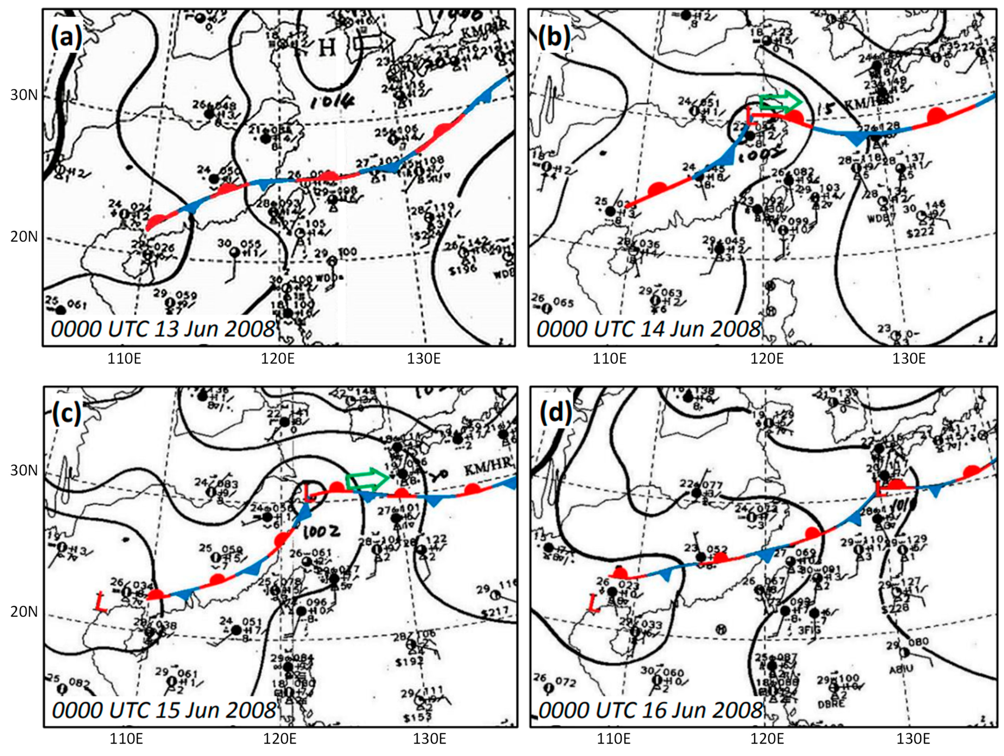
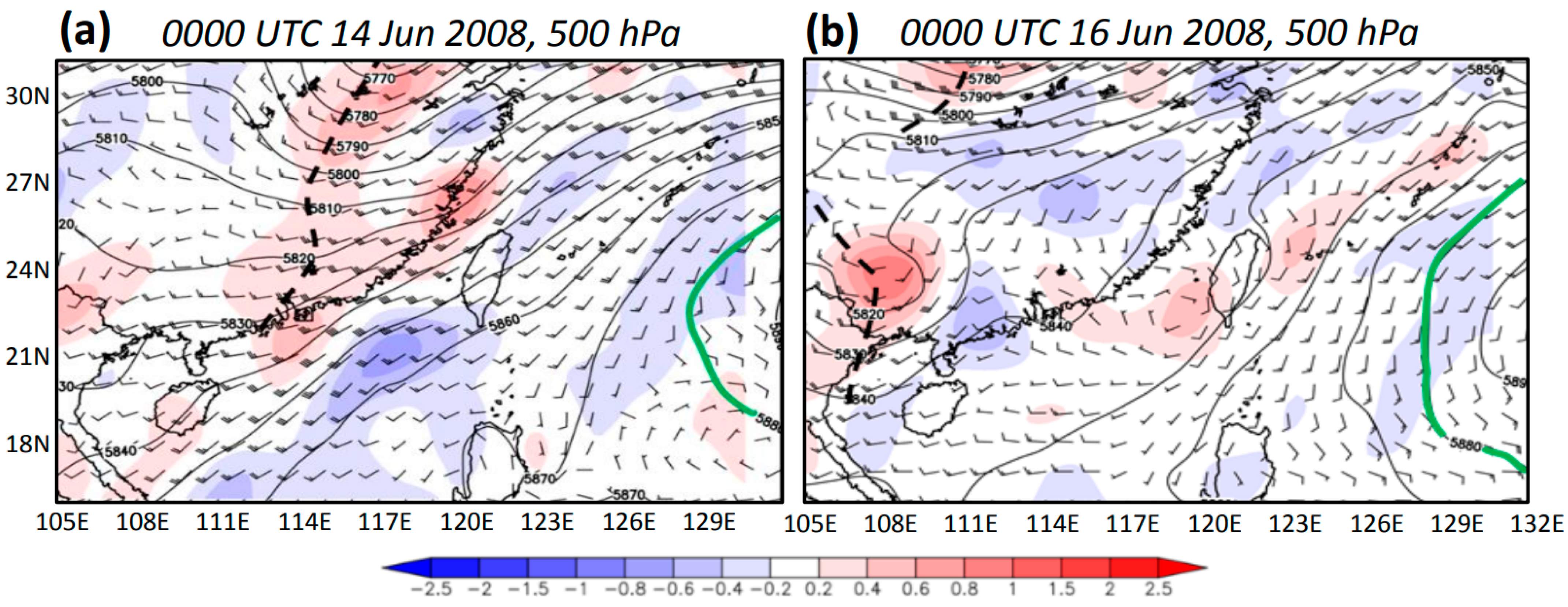
3.1. Synoptic Overview of Events A and B
3.2. Mesoscale Aspects of Event A
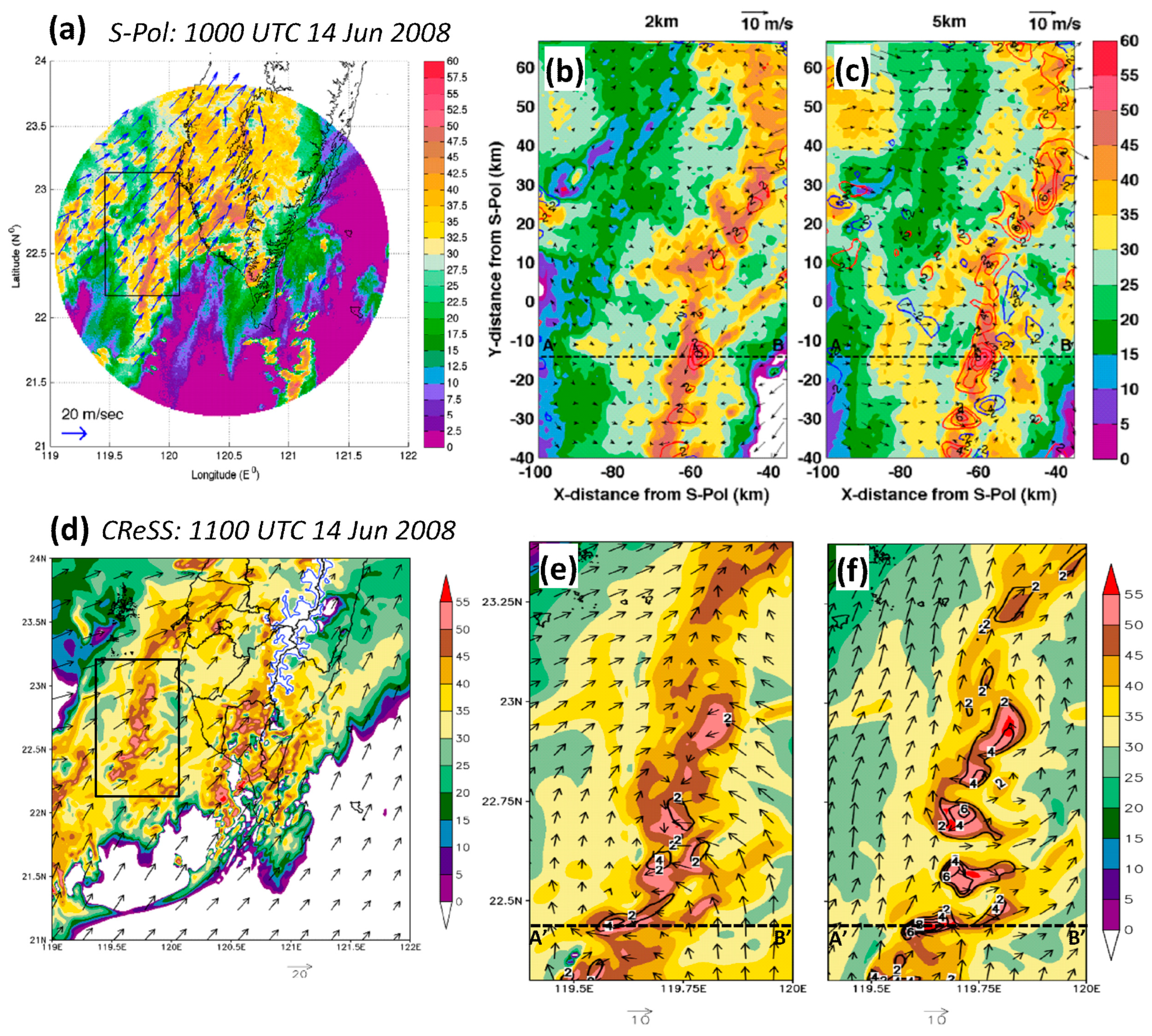
3.3. S-Pol Radar Observations of Event A
3.4. Model Results of Event A and Comparison with Radar Observations
4. The SWMCS Case on 16 June 2008
4.1. Mesoscale Aspects of Event B
4.2. S-Pol Radar Observations of Event B
4.3. Model Results of Event B and Comparison with Radar Observations
5. The Frontal Convection in IOP-3
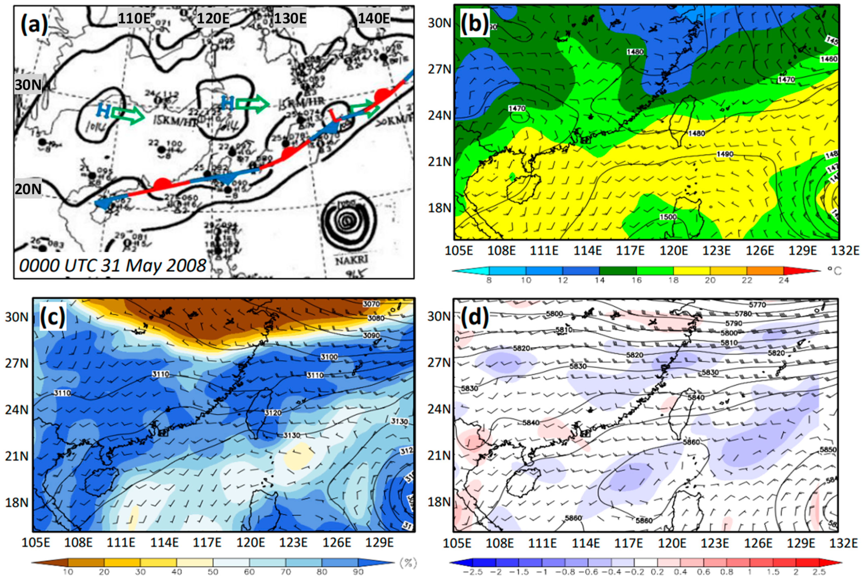
5.1. Synoptic Overview of Event C
5.2. Mesoscale Aspects of Event C
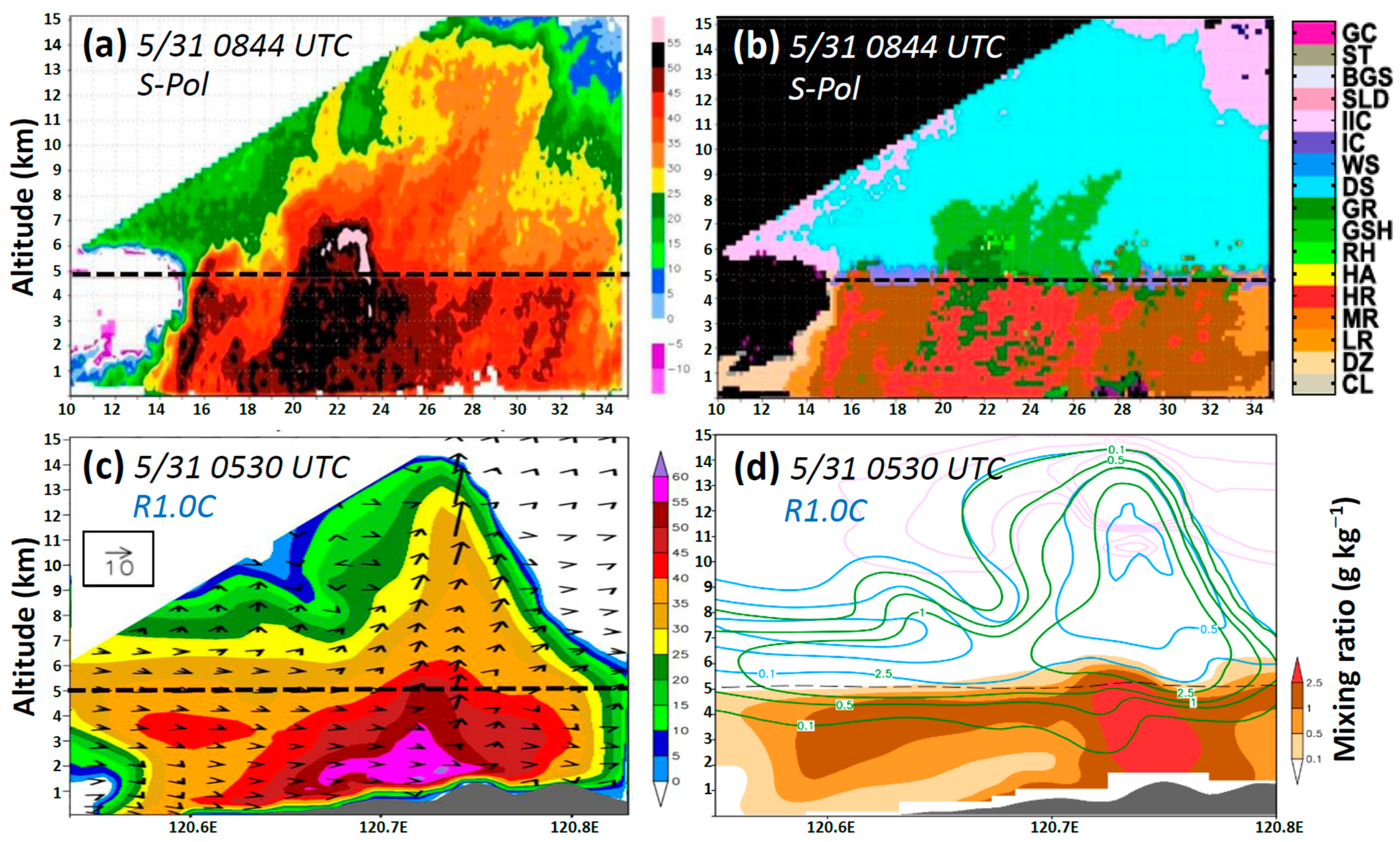
5.3. S-Pol Radar Observations of Event C
5.4. Model Results and Comparison with Radar Observations
6. Conclusions and Summary
Author Contributions
Funding
Data Availability Statement
Acknowledgments
Conflicts of Interest
References
- Chen, G.T.-J. Research on the phenomena of Meiyu during the past quarter century: An overview. In East Asian Monsoon; Chang, C.-P., Ed.; World Scientific Series on Asia-Pacific Weather and Climate: Hackensack, NJ, USA, 2004; Volume 3, pp. 357–403. [Google Scholar]
- Anthes, R.A. A cumulus parameterization scheme utilizing a one-dimensional cloud model. Mon. Weather Rev. 1977, 105, 270–286. [Google Scholar] [CrossRef]
- Anthes, R.A.; Warner, T.T. Development of hydrodynamic models suitable for air pollution and other meteorological studies. Mon. Weather Rev. 1978, 106, 1045–1078. [Google Scholar] [CrossRef]
- Molinari, J.; Dudek, M. Parameterization of convective precipitation in mesoscale numerical models. A critical review. Mon. Weather Rev. 1992, 120, 326–344. [Google Scholar] [CrossRef]
- Tsuboki, K.; Sakakibara, A. Large-scale parallel computing of Cloud Resolving Storm Simulator. In High Performance Computing; Zima, H.P., Joe, K., Sato, M., Seo, Y., Shimasaki, M., Eds.; Springer: Berlin/Heidelberg, Germany, 2002; pp. 243–259. [Google Scholar]
- Bryan, G.H.; Wyngaard, J.C.; Fritsch, J.M. Resolution requirements for the simulation of deep moist convection. Mon. Weather Rev. 2003, 131, 2394–2416. [Google Scholar] [CrossRef]
- Skamarock, W.C.; Klemp, J.B.; Dudhia, J.; Gill, D.O.; Barker, D.M.; Wang, W.; Powers, J.G. A Description of the Advanced Research WRF Version 2; University Corporation for Atmospheric Research: Boulder, CO, USA, 2005; 100p. [Google Scholar]
- Lin, Y.-L.; Farley, R.D.; Orville, H.D. Bulk parameterization of the snow field in a cloud model. J. Appl. Meteorol. Climatol. 1983, 22, 1065–1092. [Google Scholar] [CrossRef]
- Straka, J.M.; Mansell, E.R. A bulk microphysics parameterization with multiple ice precipitation categories. J. Appl. Meteorol. Climatol. 2005, 44, 445–466. [Google Scholar] [CrossRef]
- Gentry, M.S.; Lackmann, G.M. Sensitivity of simulated tropical cyclone structure and intensity to horizontal resolution. Mon. Weather Rev. 2010, 138, 688–704. [Google Scholar] [CrossRef]
- Wang, C.-C.; Kuo, H.-C.; Chen, Y.-H.; Huang, H.-L.; Chung, C.-H.; Tsuboki, K. Effects of asymmetric latent heating on typhoon movement crossing Taiwan: The case of Morakot (2009) with extreme rainfall. J. Atmos. Sci. 2012, 69, 3172–3196. [Google Scholar] [CrossRef]
- Wang, C.-C.; Hsu, J.C.-S.; Chen, G.T.-J.; Lee, D.-I. A study of two propagating heavy-rainfall episodes near Taiwan during SoWMEX/TiMREX IOP-8 in June 2008. Part I: Synoptic evolution, episode propagation, and model control simulation. Mon. Weather Rev. 2014, 142, 2619–2643. [Google Scholar] [CrossRef]
- Luo, X.; Fei, J.; Huang, X.; Ding, J.; Ma, Z. Relative roles of dry intrusion, latent heat and instabilities in the Mei-yu rainband life cycle: A case study. Atmos. Res. 2018, 214, 10–20. [Google Scholar] [CrossRef]
- Knupp, K.R.; Cotton, W.R. An Intense, Quasi-steady thunderstorm over mountainous terrain. Part II: Doppler radar observations of the storm morphological structure. J. Atmos. Sci. 1982, 39, 343–358. [Google Scholar] [CrossRef]
- Rutledge, S.A.; Hobbs, P.V. The mesoscale and microscale structure and organization of clouds and precipitation in mid latitude clouds. Part XII: A diagnostic modeling study of precipitation development in narrow cold frontal rainbands. J. Atmos. Sci. 1984, 41, 2949–2972. [Google Scholar] [CrossRef]
- Cotton, W.R.; Tripoli, G.J.; Rauber, R.M.; Mulvihill, E.A. Numerical simulation of the effects of varying ice crystal nucleation rates and aggregation processes on orographic snowfall. J. Appl. Meteorol. Climatol. 1986, 25, 1658–1680. [Google Scholar] [CrossRef]
- Yoshizaki, M. Numerical simulations of tropical squall-line clusters: Two-dimensional model. J. Meteor. Soc. Jpn. Ser. II 1986, 64, 469–491. [Google Scholar] [CrossRef]
- Fovell, R.G.; Ogura, Y. Numerical simulation of a midlatitude squall line in two dimensions. J. Atmos. Sci. 1988, 45, 3846–3879. [Google Scholar] [CrossRef]
- Tao, W.-K.; Simpson, J. Modeling study of a tropical squall-type convective line. J. Atmos. Sci. 1989, 46, 177–202. [Google Scholar] [CrossRef]
- Wang, Y. An explicit simulation of tropical cyclones with a triply nested movable mesh primitive equation model: TCM3. Part II: Model refinements and sensitivity to cloud microphysics parameterization. Mon. Weather Rev. 2002, 130, 3022–3036. [Google Scholar] [CrossRef]
- Zhu, T.; Zhang, D.-L. Numerical simulation of Hurricane Bonnie (1998). Part II: Sensitivity to varying cloud microphysical processes. J. Atmos. Sci. 2006, 63, 109–126. [Google Scholar] [CrossRef]
- Tao, W.-K.; Scale, J.R.; Ferrier, B.; Simpson, J. The effect of melting processes on the development of a tropical and a midlatitude squall line. J. Atmos. Sci. 1995, 52, 1934–1948. [Google Scholar] [CrossRef]
- Vivekanandan, J.; Ellis, S.M.; Oye, R.; Zrnic, D.S.; Ryzhkov, A.V.; Straka, J. Cloud microphysics retrieval using S-band dual-polarization radar measurements. Bull. Am. Meteorol. Soc. 1999, 80, 381–388. [Google Scholar] [CrossRef]
- Aydin, K.; Seliga, T.A.; Balaji, V. Remote sensing of hail with a dual linear polarization radar. J. Appl. Meteorol. Climatol. 1986, 25, 1475–1484. [Google Scholar] [CrossRef]
- Doviak, R.J.; Zrnic, D.S. Doppler Radar and Weather Observations; Academic Press: Cambridge, MA, USA, 1993; p. 562. [Google Scholar]
- Straka, J.M.; Zrnic, D.S. An algorithm to deduce hydrometeor types and contents from multiparameter radar data. Preprints. In Proceedings of the 26th International Conference on Radar Meteorology, Norman, OK, USA, 24–28 May 1993; American Meteorological Society: Boston, MA, USA, 1993; pp. 513–515. [Google Scholar]
- Vivekanandan, J.; Bringi, V.N.; Raghavan, R. Multiparameter radar modeling and observations of melting ice. J. Atmos. Sci. 1990, 47, 549–564. [Google Scholar] [CrossRef]
- Zrnic, D.S.; Balakrishnan, N.; Ziegler, C.L.; Bringi, V.N.; Aydin, K.; Matejka, T. Polarimetric signatures in the stratiform region of a mesoscale convective system. J. Appl. Meteor. 1993, 32, 678–693. [Google Scholar] [CrossRef]
- Vivekanandan, J.; Bringi, V.N.; Hagen, M.; Meischner, P. Polarimetric radar studies of atmospheric ice particles. IEEE Trans. Geosci. Remote Sens. 1994, 32, 1–10. [Google Scholar] [CrossRef]
- Aydin, K.V.; Bringi, N.; Liu, L. Rain-rate estimation in the presence of hail using S-band specific differential phase and other radar parameters. J. Appl. Meteorol. Climatol. 1995, 34, 404–410. [Google Scholar] [CrossRef]
- Hall, M.P.M.; Goddard, J.W.F.; Cherry, S.M. Identification of hydrometeors and other targets by dual-polarization radar. Radio Sci. 1984, 19, 132–140. [Google Scholar] [CrossRef]
- Hendry, A.; Antar, Y.M.M. Precipitation particle identification with centimeter wavelength dual-polarization radar. Radio Sci. 1984, 19, 115–122. [Google Scholar] [CrossRef]
- Lopez, R.E.; Aubagnac, J.P. The lightning activity of a hailstorm as a function of changes in its microphysical characteristics inferred from polarimetric radar observations. J. Geophys. Res. 1997, 102, 16799–16813. [Google Scholar] [CrossRef]
- May, P.T.; Keenan, T.D. Four-dimensional microphysical data from Darwin. In Proceedings of the 13th ARM Science Team Meeting Proceedings, Broomfield, CO, USA, 31 March–4 April 2003. [Google Scholar]
- Jou, B.J.-D.; Lee, W.-C.; Johnson, R.H. An overview of SoWMEX/TiMREX. In The Global Monsoon System: Research and Forecast, 2nd ed.; Chang, C.-P., Ding, Y., Lau, N.-C., Johnson, R.H., Wang, B., Eds.; World Scientific Series on Asia-Pacific Weather and Climate: Hackensack, NJ, USA, 2011; Volume 5, pp. 303–318. [Google Scholar]
- Zhou, J.-Y. Observational Analysis and Numerical Simulation of SoWMEX (IOP-8): The Characteristics of the Microphysical Structure and Compared to Microphysics Schemes. Master’s Thesis, Dept. of Atmospheric Sciences, National Central Univ., Taoyuan, Taiwan, 2012. (In Chinese with English abstract). [Google Scholar]
- Tsuboki, K.; Sakakibara, A. Numerical Prediction of High-Impact Weather Systems: The Textbook for the Seventeenth IHP Training Course in 2007; Hydrospheric Atmospheric Research Center, Nagoya University, and UNESCO: Nagoya, Japan, 2007; 273p. [Google Scholar]
- Wang, C.-C.; Chen, Y.-H.; Li, M.-C.; Kuo, H.-C.; Tsuboki, K. On the separation of upper and low-level centres of tropical storm Kong-Rey (2013) near Taiwan in association with asymmetric latent heating. Q. J. R. Meteorol. Soc. 2021, 147, 1135–1149. [Google Scholar] [CrossRef]
- Wang, C.-C.; Hsu, J.C.-S.; Chen, G.T.-J.; Lee, D.-I. A study of two propagating heavy-rainfall episodes near Taiwan during SoWMEX/TiMREX IOP-8 in June 2008. Part II: Sensitivity tests on the roles of synoptic conditions and topographic effects. Mon. Weather Rev. 2014, 142, 2644–2664. [Google Scholar] [CrossRef]
- Wang, C.-C.; Chiou, B.-K.; Chen, G.T.-J.; Kuo, H.-C.; Liu, C.-H. A numerical study of back-building process in a quasistationary rainband with extreme rainfall over northern Taiwan during 11–12 June 2012. Atmos. Chem. Phys. 2016, 16, 12359–12382. [Google Scholar] [CrossRef]
- Wang, C.-C.; Kuo, H.-C.; Yeh, T.-C.; Chung, C.-H.; Chen, Y.-H.; Huang, S.-Y.; Wang, Y.-W.; Liu, C.-H. High-resolution quantitative precipitation forecasts and simulations by the Cloud-Resolving Storm Simulator (CReSS) for Typhoon Morakot (2009). J. Hydrol. 2013, 506, 26–41. [Google Scholar] [CrossRef]
- Wang, C.-C.; Li, M.-S.; Chang, C.-S.; Chuang, P.-Y.; Chen, S.-H.; Tsuboki, K. Ensemble-based sensitivity analysis and predictability of an extreme rainfall event over northern Taiwan in the Mei-Yu season: The 2 June 2017 case. Atmos. Res. 2021, 259, 105684. [Google Scholar] [CrossRef]
- Wang, C.-C.; Yeh, T.-Y.; Chang, C.-S.; Li, M.-S.; Tsuboki, K.; Liu, C.-H. A modeling study of an extreme rainfall event along the northern coast of Taiwan on 2 June 2017. Atmos. Chem. Phys. 2023, 23, 501–521. [Google Scholar] [CrossRef]
- Wang, C.-C.; Tsai, C.-H.; Jou, B.J.-D.; David, S.J. Time-lagged ensemble quantitative precipitation forecasts for three landfalling typhoons in the Philippines using the CReSS Model, Part I: Description and verification against rain-gauge observations. Atmosphere 2022, 13, 1193. [Google Scholar] [CrossRef]
- Murakami, M.; Clark, T.L.; Hall, W.D. Numerical simulations of convective snow clouds over the sea of Japan; Two-dimensional simulations of mixed layer development and convective snow cloud formation. J. Meteor. Soc. Japan 1994, 72, 43–62. [Google Scholar] [CrossRef]
- Chang, W.-Y.; Lee, W.-C.; Liou, Y.-C. The kinematic and microphysical characteristics and associated precipitation efficiency of subtropical convection during SoWMEX/TiMREX. Mon. Weather Rev. 2015, 143, 317–340. [Google Scholar] [CrossRef]
- Tseng, Y.-S. Frontal Convection Analysis Using SPOL Radar during SoWMEX. Master’s Thesis, Department of Environmental Information and Engineering, Chung-Cheng Institute Technology, National Defense University, Taoyuan, Taiwan, 2013. [Google Scholar]
- Murakami, M. Numerical modeling of dynamical and microphysical evolution of an isolated convective cloud: The 19 July 1981 CCOPE cloud. J. Meteor. Soc. Jpn. 1990, 68, 107–128. [Google Scholar] [CrossRef]
- Ikawa, M.; Saito, K. Description of a nonhydrostatic model developed at the forecast research department of the MRI. Tech. Rep. MRI 1991, 28, 238. [Google Scholar]
- Deardorff, J.W. Stratocumulus-capped mixed layers derived from a three-dimensional model. Bound.-Layer Meteor. 1980, 18, 495–527. [Google Scholar] [CrossRef]
- Kondo, J. Heat balance of the China Sea during the air mass transformation experiment. J. Meteor. Soc. Jpn. 1976, 54, 382–398. [Google Scholar] [CrossRef]
- Louis, J.F.; Tiedtke, M.; Geleyn, J.F. A Short History of the Operational PBL Parameterization at ECMWF. In Workshop on Planetary Boundary Layer Parameterization; ECMWF: Reading, UK, 1982; pp. 59–79. [Google Scholar]
- Segami, A.; Kurihara, K.; Nakamura, H.; Ueno, M.; Takano, I.; Tatsumi, Y. Operational mesoscale weather prediction with Japan spectral model. J. Meteor. Soc. Jpn. 1989, 67, 907–924. [Google Scholar] [CrossRef]
- Wang, C.-C.; Huang, S.-Y.; Chen, S.-H.; Chang, C.-S.; Tsuboki, K. Cloud-resolving typhoon rainfall ensemble forecasts for Taiwan with large domain and extended range through time-lagged approach. Wea. Forecast. 2016, 31, 151–172. [Google Scholar] [CrossRef]
- Wang, C.-C.; Chang, C.-S.; Wang, Y.-W.; Huang, C.-C.; Wang, S.-C.; Chen, Y.-S.; Tsuboki, K.; Huang, S.-Y.; Chen, S.-H.; Chuang, P.-Y.; et al. Evaluating quantitative precipitation forecasts using the 2.5 km CReSS model for typhoons in Taiwan: An update through the 2015 season. Atmosphere 2021, 12, 1501. [Google Scholar] [CrossRef]
- Wang, C.-C.; Chuang, P.-Y.; Chang, C.-S.; Tsuboki, K.; Huang, S.-Y.; Leu, G.-C. Evaluation of Mei-yu heavy-rainfall quantitative precipitation forecasts in Taiwan by a cloud-resolving model for three seasons of 2012-2014. Nat. Hazards Earth Syst. Sci. 2022, 22, 23–40. [Google Scholar] [CrossRef]
- Chen, X.A.; Chen, Y.-L. Development of low-level jets during TAMEX. Mon. Weather Rev. 1995, 123, 1695–1719. [Google Scholar] [CrossRef]
- Xu, W.; Zipser, E.J.; Chen, Y.-L.; Liu, C.; Liou, Y.-C.; Lee, W.-C.; Jou, B.J.-D. An orography-associated extreme rainfall event during TiMREX: Initiation, storm evolution, and maintenance. Mon. Weather Rev. 2012, 140, 2555–2574. [Google Scholar] [CrossRef]
- Davis, C.A.; Lee, W.-C. Mesoscale analysis of heavy rainfall episodes from SoWMEX/TiMREX. J. Atmos. Sci. 2012, 69, 521–537. [Google Scholar] [CrossRef]
- Tu, C.-C.; Chen, Y.-L.; Chen, C.-S.; Lin, P.-L.; Lin, P.-H. A comparison of two heavy rainfall events during the terrain-influenced monsoon rainfall experiment (TiMREX) 2008. Mon. Weather Rev. 2014, 142, 2436–2463. [Google Scholar] [CrossRef]


| Projection | Lambert Conformal, Center at 120°E, Secant at 10°N and 40°N |
|---|---|
| Topography data | Digital elevation model at intervals of (1/120)° |
| Cloud microphysics | Double-moment bulk cold-rain scheme |
| PBL turbulence | 1.5-order closure with turbulent kinetic energy prediction |
| Surface processes | Momentum/energy fluxes and shortwave and longwave radiation |
| Substrate model | 43 levels, every 5 cm to 2.1 m in depth |
| Event Name | Event A | Event B | Event C |
|---|---|---|---|
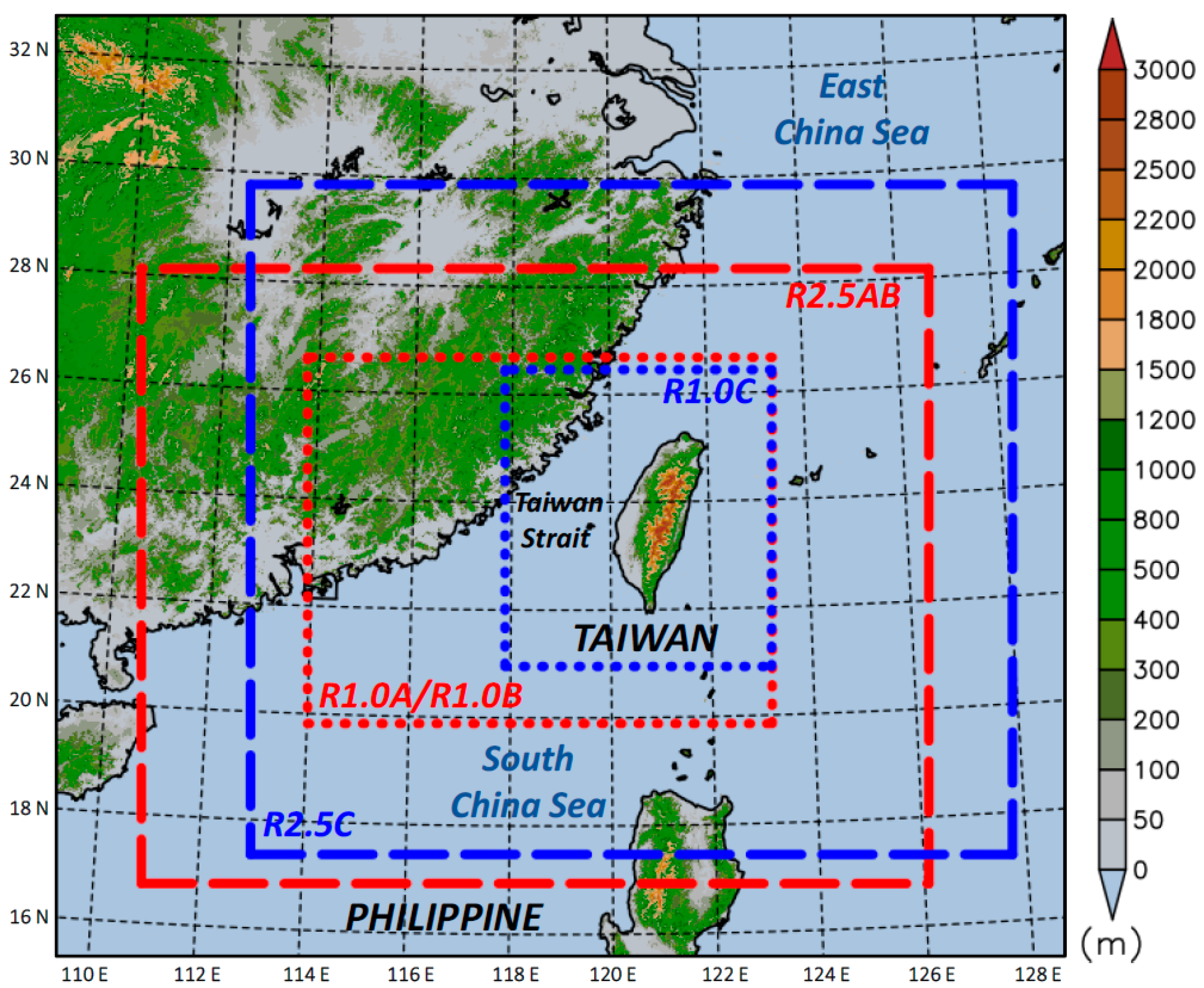
| Experiment name (2.5 km) | R2.5AB | R2.5C | |
| Grid spacing (km) | 2.5 × 2.5 × 0.5 * | ||
| Grid dimension (x × y × z) | 600 × 480 × 40 | 585 × 520 × 60 | |
| Domain size (km) | 1500 × 1200 × 20 | 1455 × 1305 × 30 | |
| Initial time | 0000 UTC 12 June | 0000 UTC 30 May | |
| Integration length and output frequency | 144 h, 30 min | 48 h, 15 min | |
| IC/BCs | NCEP GFS final analyses (1° × 1°, 26 levels, every 6 h) | ||
| Experiment name (1 km) | R1.0A | R1.0B | R1.0C |
| Grid spacing (km) | 1.0 × 1.0 × 0.5 * | ||
| Grid dimension (x × y × z) | 900 × 720 × 37 | 528 × 549 × 56 | |
| Domain size (km) | 900 × 720 × 18.5 | 528 × 549 × 28 | |
| Initial time | 0000 UTC 13 June | 1800 UTC 15 June | 2100 UTC 30 May |
| Forecast range and interval | 48 h, 15 min | 22 h, 15 min | 18 h, 5 min |
| IC/BCs | Outputs of R2.5AB | Outputs of R2.5C | |
Disclaimer/Publisher’s Note: The statements, opinions and data contained in all publications are solely those of the individual author(s) and contributor(s) and not of MDPI and/or the editor(s). MDPI and/or the editor(s) disclaim responsibility for any injury to people or property resulting from any ideas, methods, instructions or products referred to in the content. |
© 2023 by the authors. Licensee MDPI, Basel, Switzerland. This article is an open access article distributed under the terms and conditions of the Creative Commons Attribution (CC BY) license (https://creativecommons.org/licenses/by/4.0/).
Share and Cite
Wang, C.-C.; Chen, Y.-H.; Lan, Y.-Y.; Chang, W.-Y. An Evaluation of Simulated Cloud Microphysical Characteristics of Three Mei-Yu Rainfall Systems in Taiwan by a Cloud-Resolving Model Using Dual-Polarimetric Radar Observations. Remote Sens. 2023, 15, 4651. https://doi.org/10.3390/rs15194651
Wang C-C, Chen Y-H, Lan Y-Y, Chang W-Y. An Evaluation of Simulated Cloud Microphysical Characteristics of Three Mei-Yu Rainfall Systems in Taiwan by a Cloud-Resolving Model Using Dual-Polarimetric Radar Observations. Remote Sensing. 2023; 15(19):4651. https://doi.org/10.3390/rs15194651
Chicago/Turabian StyleWang, Chung-Chieh, Yu-Han Chen, Yu-Yao Lan, and Wei-Yu Chang. 2023. "An Evaluation of Simulated Cloud Microphysical Characteristics of Three Mei-Yu Rainfall Systems in Taiwan by a Cloud-Resolving Model Using Dual-Polarimetric Radar Observations" Remote Sensing 15, no. 19: 4651. https://doi.org/10.3390/rs15194651