
Urban Vegetation Extraction from High-Resolution Remote Sensing Imagery on SD-UNet and Vegetation Spectral Features
 ,
,  ,
,
Abstract
:1. Introduction
- An optimized convolutional neural network (SD-UNet) was proposed to effectively extract urban vegetation from Gaofen-1 remote sensing images.
- Three sample sets were established to evaluate the influence of the vegetation spectral features on the model extraction results. The SD-UNet was trained on three sample sets, finally obtaining the best model.
- The SD-UNet’s performance on urban vegetation extraction was compared with U-Net, SegNet, NDVI, and RF. The SD-UNet trained on three sample sets was applied to four scenes and the best model was applied to two administrative divisions to evaluate their generalization ability in vegetation extraction.
2. Materials and Methods
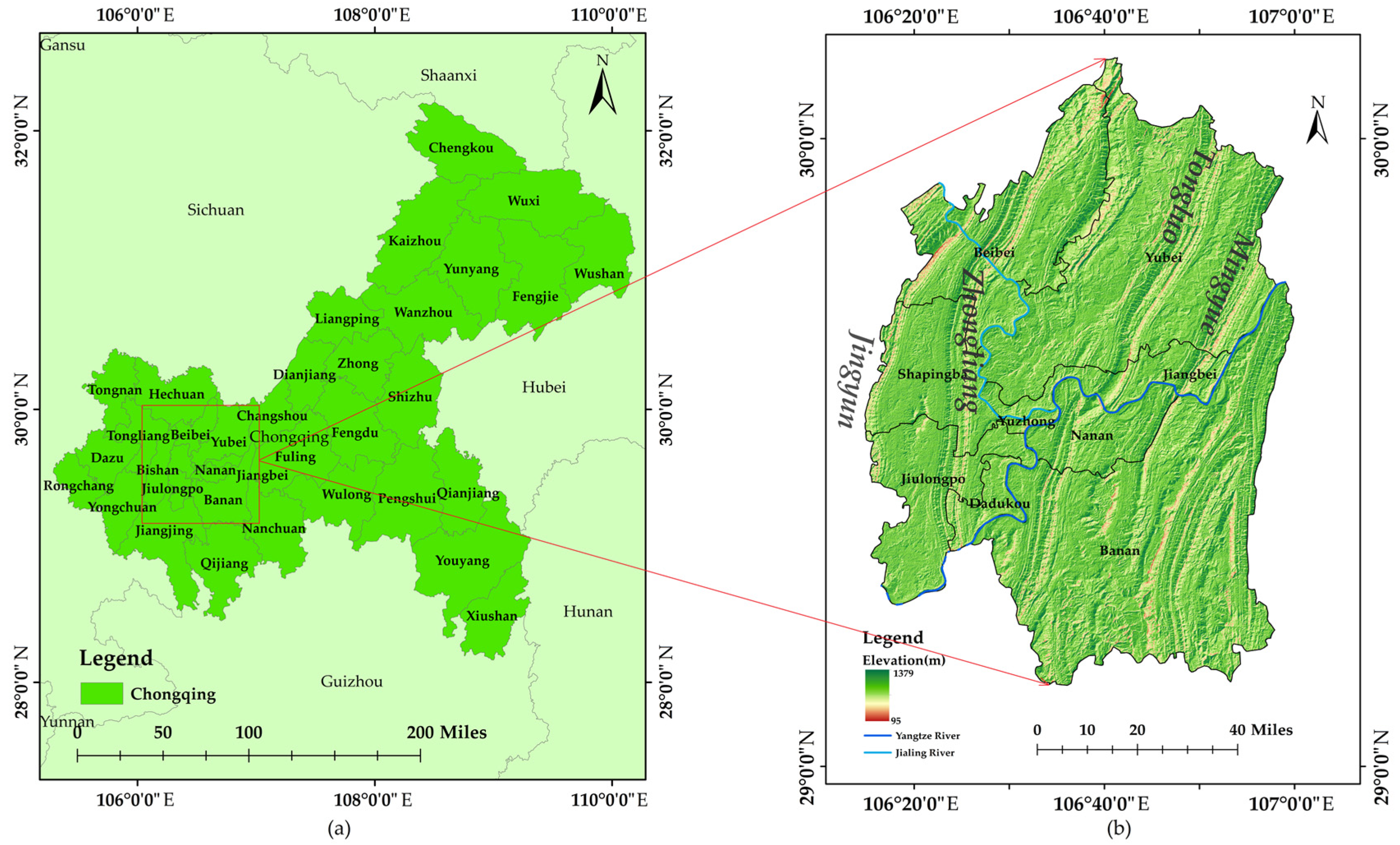
2.1. Study Area and Data Sources
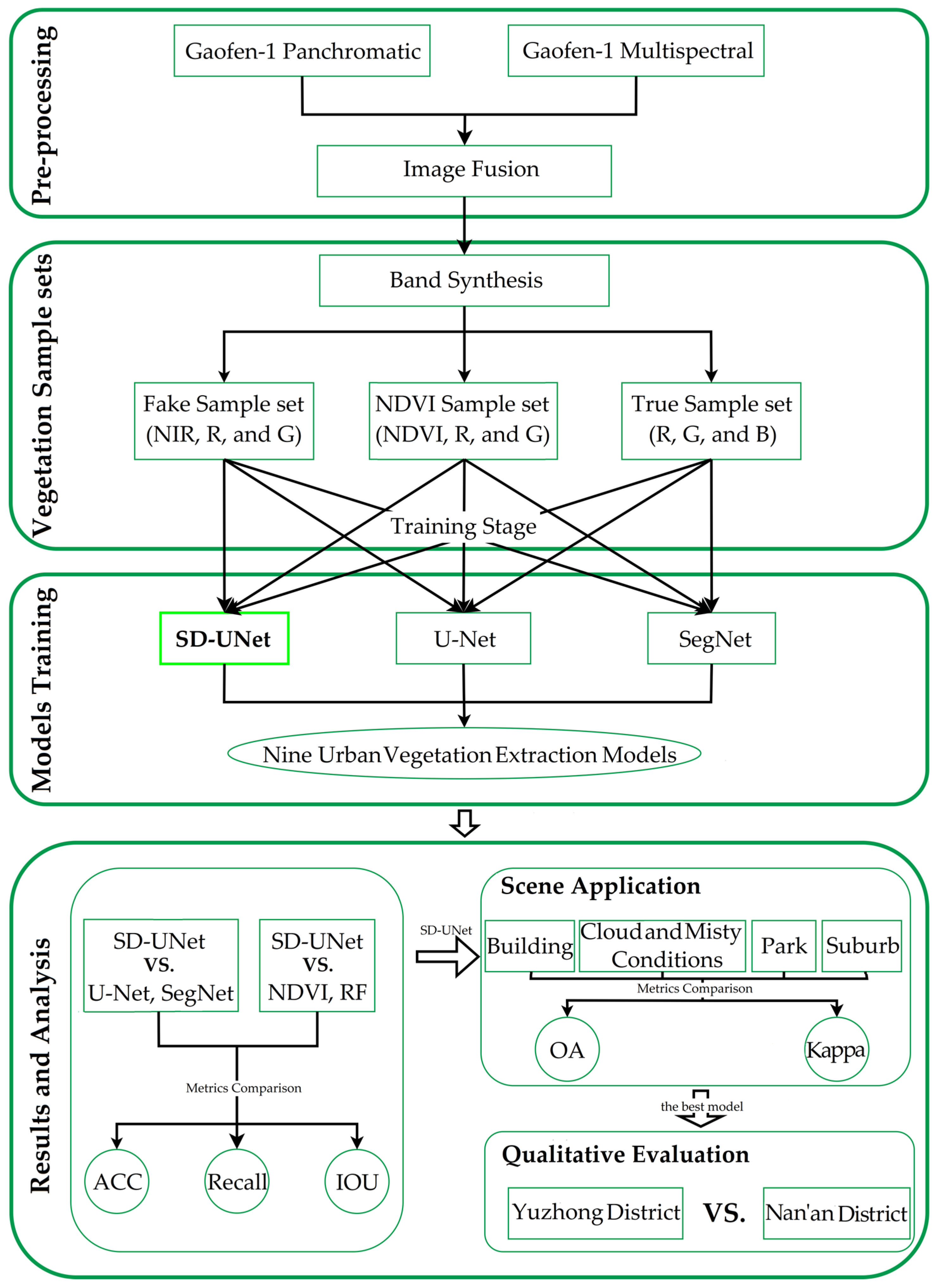
2.2. Experimental Process
2.3. Sample Sets
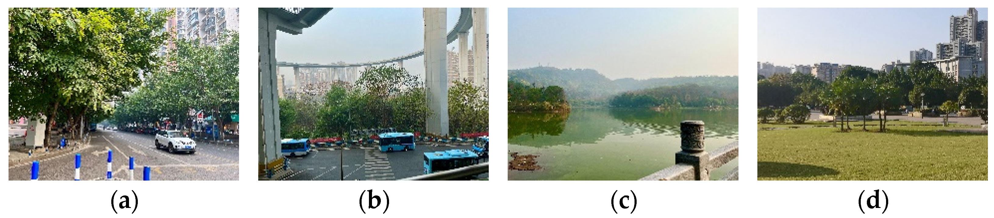
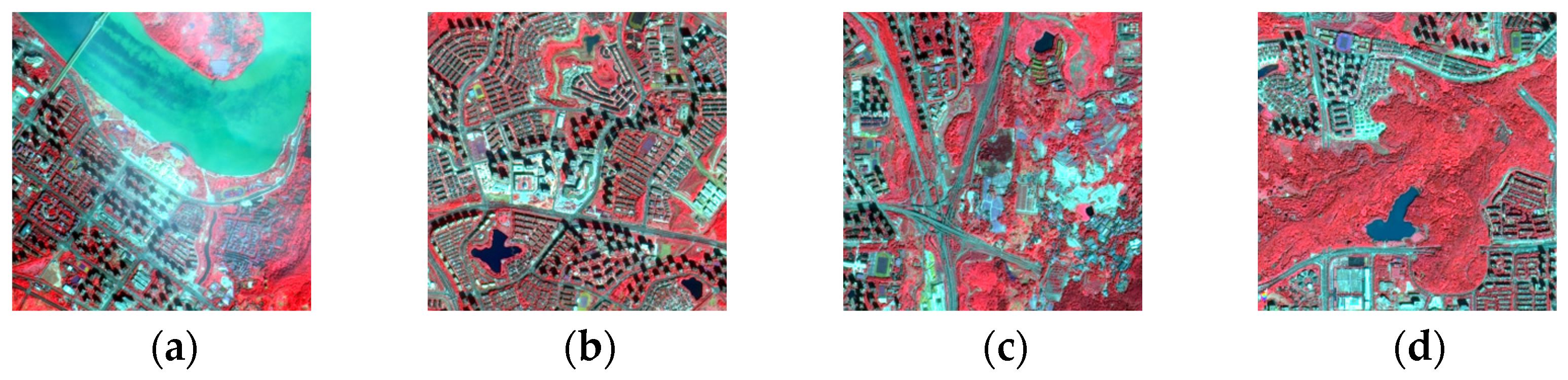
2.4. Scene Data
2.5. Methods
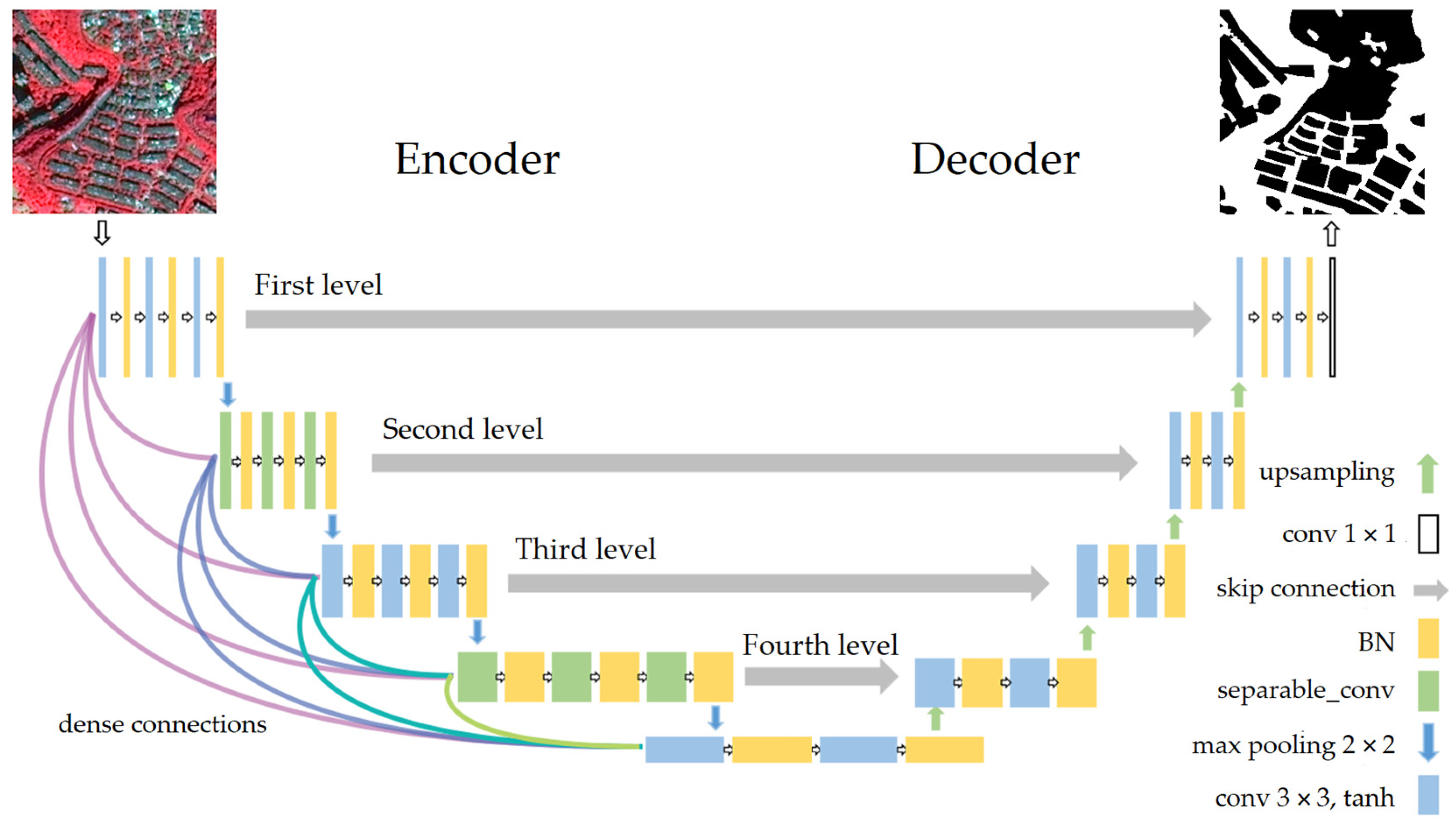
2.5.1. SD-UNet Model
2.5.2. Experimental Environment
2.5.3. Assessment Measures
3. Results and Analysis
3.1. Results
3.1.1. SD-UNet Results
3.1.2. NDVI Results
3.1.3. Random Forest Results
3.2. Analysis
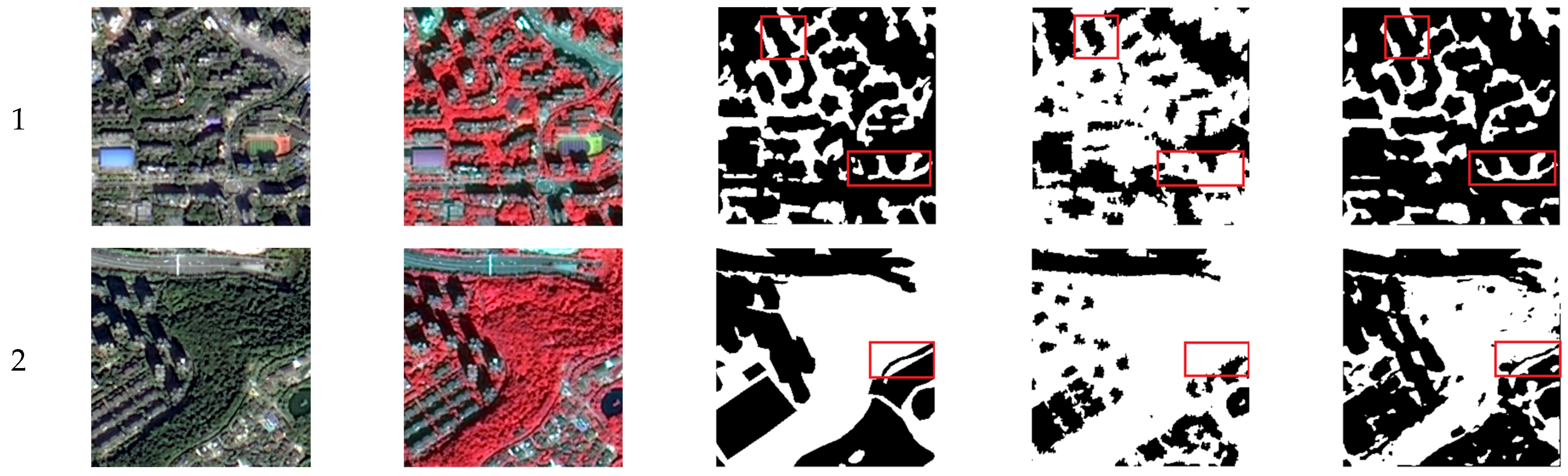
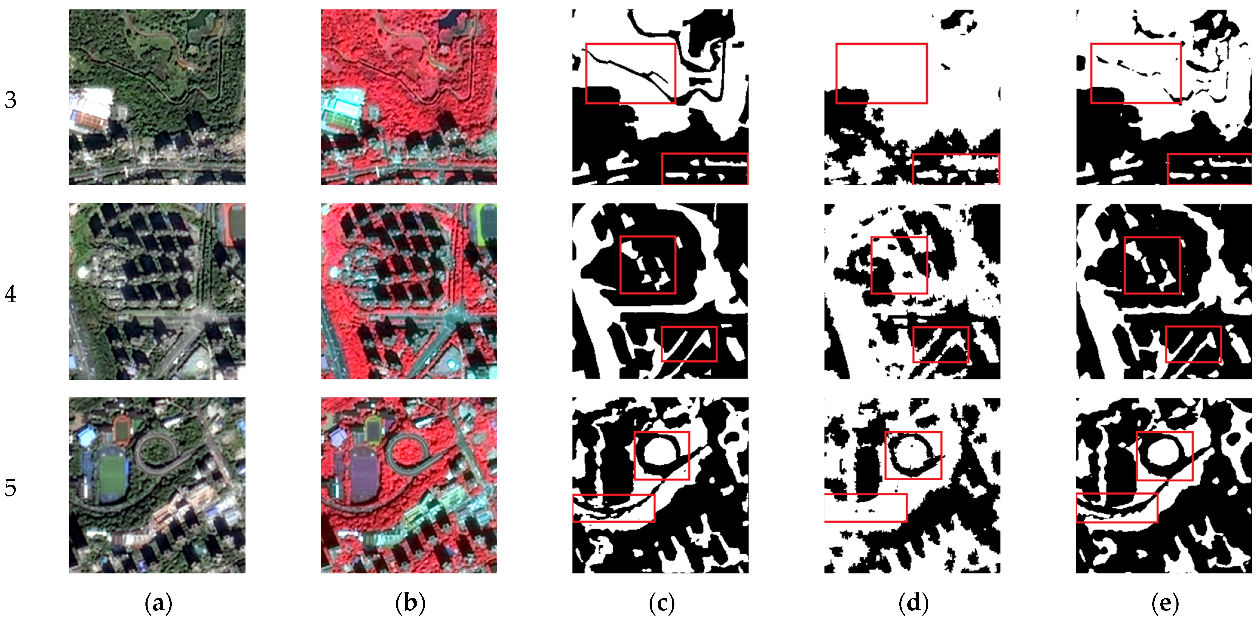
3.2.1. SD-UNet vs. U-Net, SegNet
3.2.2. SD-UNet vs. RF, NDVI
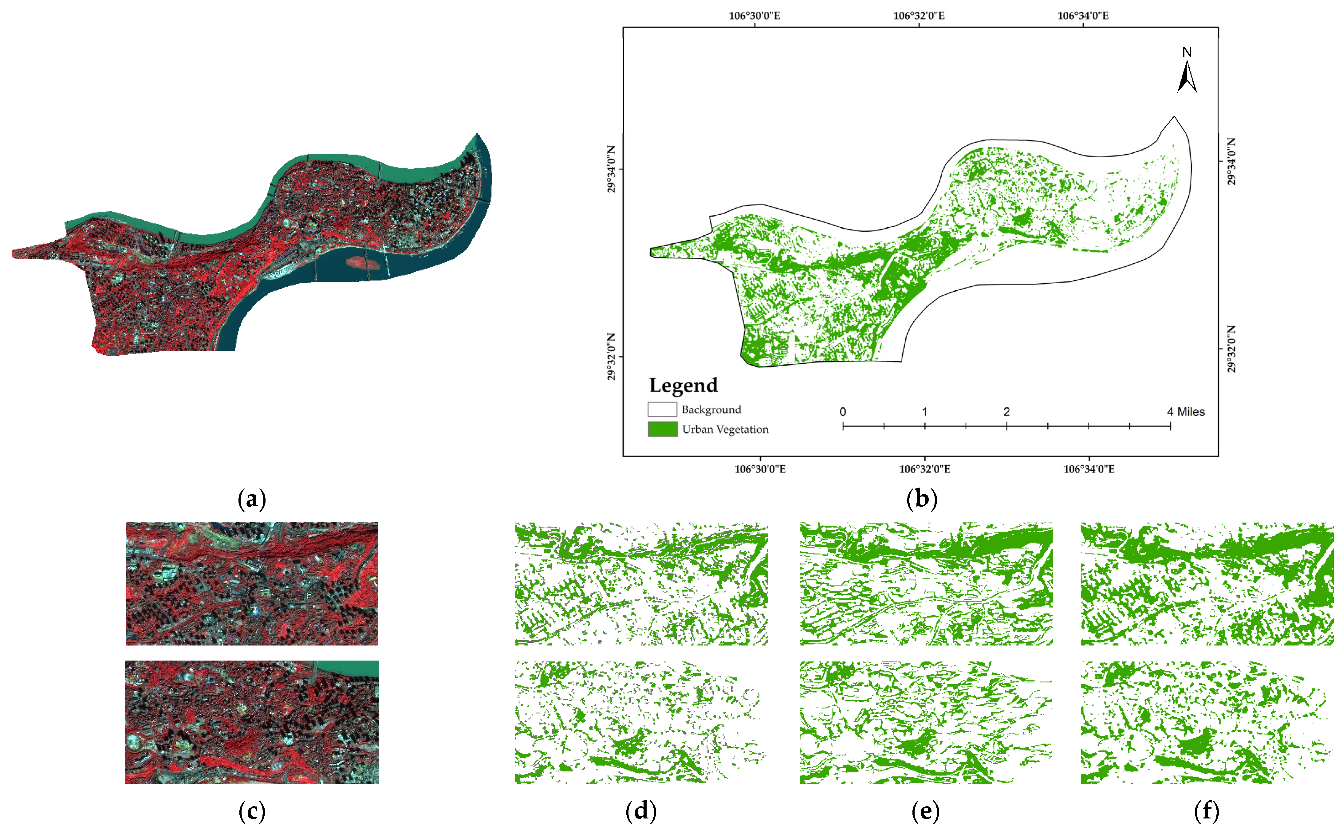
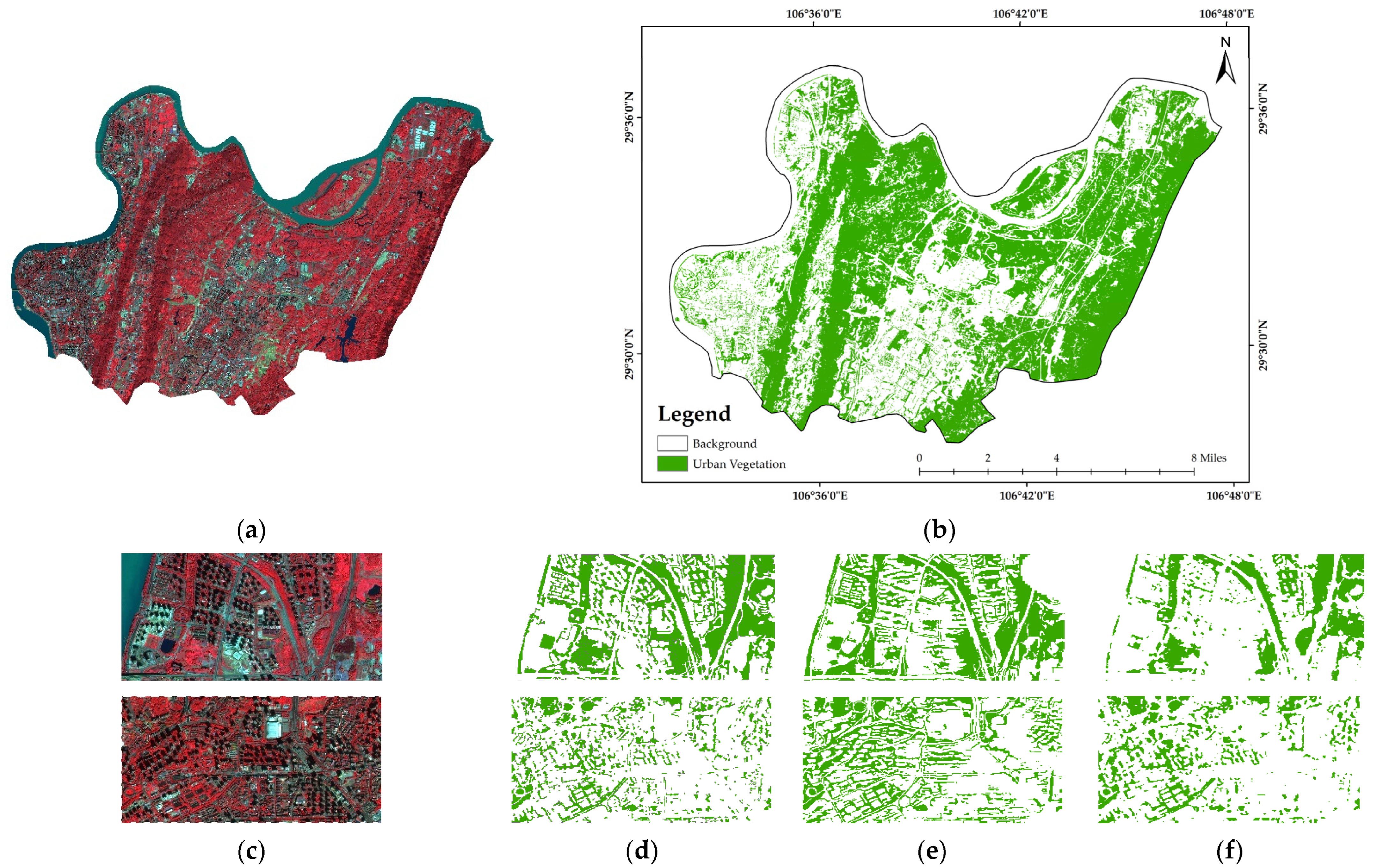
3.3. Scene Application
3.4. Qualitative Evaluation of Administrative Divisions
4. Discussion
4.1. Sample Set Evaluation
4.2. SD-UNet’s Superiority in the Structure
4.3. SD-UNet’s Applicability
5. Conclusions
Author Contributions
Funding
Data Availability Statement
Conflicts of Interest
References
- Abdollahi, A.; Pradhan, B. Urban Vegetation Mapping from Aerial Imagery Using Explainable AI (XAI). Sensors 2021, 21, 4738. [Google Scholar] [CrossRef] [PubMed]
- Guo, J.H.; Xu, Q.S.; Zeng, Y.; Liu, Z.H.; Zhu, X.X. Nationwide urban tree canopy mapping and coverage assessment in Brazil from high-resolution remote sensing images using deep learning. ISPRS J. Photogramm. Remote Sens. 2023, 198, 1–15. [Google Scholar] [CrossRef]
- Xing, Y.; Brimblecombe, P. Role of vegetation in deposition and dispersion of air pollution in urban parks. Atmos. Environ. 2019, 201, 73–83. [Google Scholar] [CrossRef]
- Zheng, T.; Jia, Y.P.; Zhang, S.J.; Li, X.B.; Wu, Y.; Wu, C.L.; He, H.D.; Peng, Z.R. Impacts of vegetation on particle concentrations in roadside environments. Environ. Pollut. 2021, 282, 117067. [Google Scholar] [CrossRef]
- Lee, E.S.; Ranasinghe, D.R.; Ahangar, F.E.; Amini, S.; Mara, S.; Choi, W.; Paulson, S.; Zhu, Y. Field evaluation of vegetation and noise barriers for mitigation of near-freeway air pollution under variable wind conditions. Atmos. Environ. 2018, 175, 92–99. [Google Scholar] [CrossRef]
- Threlfall, C.G.; Mata, L.; Mackie, J.A.; Hahs, A.K.; Stork, N.E.; Williams, N.S.G.; Livesley, S.J. Increasing biodiversity in urban green spaces through simple vegetation interventions. J. Appl. Ecol. 2017, 54, 1874–1883. [Google Scholar] [CrossRef]
- Paiva, P.F.P.R.; Ruivo, M.D.P.; da Silva, O.M.; Maciel, M.D.M.; Braga, T.G.M.; de Andrade, M.M.N.; dos Santos, P.C.; da Rocha, E.S.; de Freitas, T.P.M.; Leite, T.V.D.; et al. Deforestation in protect areas in the Amazon: A threat to biodiversity. Biodivers. Conserv. 2020, 29, 19–38. [Google Scholar] [CrossRef]
- Liu, G.; Shao, Q.; Fan, J.; Huang, H.; Liu, J.; He, J. Assessment of Restoration Degree and Restoration Potential of Key Ecosystem-Regulating Services in the Three-River Headwaters Region Based on Vegetation Coverage. Remote Sens. 2023, 15, 523. [Google Scholar] [CrossRef]
- Yan, C.H.; Guo, Q.P.; Li, H.Y.; Li, L.J.; Qiu, G.Y. Quantifying the cooling effect of urban vegetation by mobile traverse method: A local-scale urban heat island study in a subtropical megacity. Build. Environ. 2019, 169, 106541. [Google Scholar] [CrossRef]
- Susca, T.; Gaffin, S.R.; Dell’Osso, G.R. Positive effects of vegetation: Urban heat island and green roofs. Environ. Pollut. 2021, 159, 2119–2126. [Google Scholar] [CrossRef]
- Olsen, J.R.; Nicholls, N.; Mitchell, R. Are urban landscapes associated with reported life satisfaction and inequalities in life satisfaction at the city level? A cross-sectional study of 66 European cities. Soc. Sci. Med. 2019, 226, 263–274. [Google Scholar] [CrossRef] [PubMed]
- Lehmann, I.; Mathey, J.; Rossler, S.; Brauer, A.; Goldberg, V. Urban vegetation structure types as a methodological approach for identifying ecosystem services—Application to the analysis of micro-climatic effects. Ecol. Indic. 2014, 42, 58–72. [Google Scholar] [CrossRef]
- Zhou, W.; Cao, F.; Wang, G. Effects of Spatial Pattern of Forest Vegetation on Urban Cooling in a Compact Megacity. Forests 2019, 10, 282. [Google Scholar] [CrossRef]
- Du, J.Q.; Fu, Q.; Fang, S.F.; Wu, J.H.; He, P.; Quan, Z.J. Effects of rapid urbanization on vegetation cover in the metropolises of China over the last four decades. Ecol. Indic. 2019, 107, 105458. [Google Scholar] [CrossRef]
- Rast, M.; Painter, T.H. Earth Observation Imaging Spectroscopy for Terrestrial Systems: An Overview of Its History, Techniques, and Applications of Its Missions. Surv. Geophys. 2019, 40, 303–331. [Google Scholar] [CrossRef]
- Zhu, X.L.; Liu, D.S. Improving forest aboveground biomass estimation using seasonal Landsat NDVI time-series. ISPRS J. Photogramm. Remote Sens. 2015, 102, 222–231. [Google Scholar] [CrossRef]
- Yang, L.; Jia, K.; Liang, S.; Wei, X.; Yao, Y.; Zhang, X. A Robust Algorithm for Estimating Surface Fractional Vegetation Cover from Landsat Data. Remote Sens. 2017, 9, 857. [Google Scholar] [CrossRef]
- Chen, X.; Yang, Y.; Zhang, D.; Li, X.; Gao, Y.; Zhang, L.; Wang, D.; Wang, J.; Wang, J.; Huang, J. Response Mechanism of Leaf Area Index and Main Nutrient Content in Mangrove Supported by Hyperspectral Data. Forests 2023, 14, 754. [Google Scholar] [CrossRef]
- Zhang, C.; Liu, Y.; Tie, N. Forest Land Resource Information Acquisition with Sentinel-2 Image Utilizing Support Vector Machine, K-Nearest Neighbor, Random Forest, Decision Trees and Multi-Layer Perceptron. Forests 2023, 14, 254. [Google Scholar] [CrossRef]
- Mao, X.; Deng, Y.; Zhu, L.; Yao, Y. Hierarchical Geographic Object-Based Vegetation Type Extraction Based on Multi-Source Remote Sensing Data. Forests 2020, 11, 1271. [Google Scholar] [CrossRef]
- Tang, Z.; Sun, Y.; Wan, G.; Zhang, K.; Shi, H.; Zhao, Y.; Chen, S.; Zhang, X. Winter Wheat Lodging Area Extraction Using Deep Learning with Gaofen-2 Satellite Imagery. Remote Sens. 2022, 14, 4887. [Google Scholar] [CrossRef]
- Zhan, Z.Q.; Zhang, X.M.; Liu, Y.; Sun, X.; Pang, C.; Zhao, C.B. Vegetation Land Use/Land Cover Extraction From High-Resolution Satellite Images Based on Adaptive Context Inference. IEEE Access 2020, 8, 21036–21051. [Google Scholar] [CrossRef]
- Abdollahi, A.; Liu, Y.X.; Pradhan, B.; Huete, A.; Dikshit, A.; Tran, N.N. Short-time-series grassland mapping using Sentinel-2 imagery and deep learning-based architecture. Egypt. J. Remote Sens. Space Sci. 2022, 25, 673–685. [Google Scholar] [CrossRef]
- Cheng, X.M.; Liu, W.D.; Zhou, J.H.; Wang, Z.Z.; Zhang, S.Q.; Liao, S.X. Extraction of Mountain Grasslands in Yunnan, China, from Sentinel-2 Data during the Optimal Phenological Period Using Feature Optimization. Agronomy 2022, 12, 1948. [Google Scholar] [CrossRef]
- Adagbasa, E.G.; Adelabu, S.A.; Okello, T.W. Application of deep learning with stratified K-fold for vegetation species discrimination in a protected mountainous region using Sentinel-2 image. Geocarto Int. 2019, 37, 142–162. [Google Scholar] [CrossRef]
- Dai, Y.; Feng, L.; Hou, X.; Tang, J. An automatic classification algorithm for submerged aquatic vegetation in shallow lakes using Landsat imagery. Remote Sens. Environ. 2021, 260, 112459. [Google Scholar] [CrossRef]
- Hadi, H.A.; Danoedoro, P. Comparing several pixel-based classification methods for vegetation structural composition mapping using Sentinel 2A imagery in Salatiga area, Central Java. In Proceedings of the Seventh Geoinformation Science Symposium, Yogyakarta, Indonesia, 25–28 October 2021. [Google Scholar]
- Meng, X.; Shang, N.; Zhang, X.; Li, C.; Zhao, K.; Qiu, X.; Weeks, E. Photogrammetric UAV Mapping of Terrain under Dense Coastal Vegetation: An Object-Oriented Classification Ensemble Algorithm for Classification and Terrain Correction. Remote Sens. 2017, 9, 1187. [Google Scholar] [CrossRef]
- Shen, Y.; Zhang, J.; Yang, L.; Zhou, X.; Li, H.; Zhou, X. A Novel Operational Rice Mapping Method Based on Multi-Source Satellite Images and Object-Oriented Classification. Agronomy 2022, 12, 3010. [Google Scholar] [CrossRef]
- Zhao, F.; Wu, X.; Wang, S. Object-oriented Vegetation Classification Method based on UAV and Satellite Image Fusion. Procedia Comput. Sci. 2020, 174, 609–615. [Google Scholar] [CrossRef]
- Bey, A.; Jetimane, J.; Lisboa, S.N.; Ribeiro, N.; Sitoe, A.; Meyfroidt, P. Mapping smallholder and large-scale cropland dynamics with a flexible classification system and pixel-based composites in an emerging frontier of Mozambique. Remote Sens. Environ. 2020, 239, 111611. [Google Scholar] [CrossRef]
- Shen, L.L.; Jia, S. Three-Dimensional Gabor Wavelets for Pixel-Based Hyperspectral Imagery Classification. IEEE Trans. Geosci. Remote Sens. 2011, 49, 5039–5046. [Google Scholar] [CrossRef]
- Sun, Z.P.; Shen, W.M.; Wei, B.; Liu, X.M.; Su, W.; Zhang, C.; Yang, J.Y. Object-oriented land cover classification using HJ-1 remote sensing imagery. Sci. China Earth Sci. 2010, 53, 34–44. [Google Scholar] [CrossRef]
- Xu, Q.; Jin, M.T.; Guo, P. A High-Precision Crop Classification Method Based on Time-Series UAV Images. Agriculture 2023, 13, 97. [Google Scholar] [CrossRef]
- Rizayeva, A.; Nita, M.D.; Radeloff, V.C. Large-area, 1964 land cover classifications of Corona spy satellite imagery for the Caucasus Mountains. Remote Sens. Environ. 2023, 284, 113343. [Google Scholar] [CrossRef]
- Saba, F.; Zoej, M.J.V.; Mokhtarzade, M. Optimization of Multiresolution Segmentation for Object-Oriented Road Detection from High-Resolution Images. Can. J. Remote Sens. 2016, 42, 75–84. [Google Scholar] [CrossRef]
- Xu, W.C.; Lan, Y.B.; Li, Y.H.; Luo, Y.F.; He, Z.Y. Classification method of cultivated land based on UAV visible light remote sensing. Int. J. Agric. Biol. Eng. 2019, 12, 103–109. [Google Scholar] [CrossRef]
- Albawi, S.; Mohammed, T.A.; Al-Zawi, S. Understanding of a convolutional neural network. In Proceedings of the 2017 International Conference on Engineering and Technology (ICET), Antalya, Turkey, 21–23 August 2017; pp. 1–6. [Google Scholar]
- Lee, H.; Kwon, H. Going Deeper with Contextual CNN for Hyperspectral Image Classification. IEEE Trans. Image Process. 2017, 26, 4843–4855. [Google Scholar] [CrossRef]
- Zheng, C.; Hu, C.; Chen, Y.C.; Li, J.Y. A Self-Learning-Update CNN Model for Semantic Segmentation of Remote Sensing Images. IEEE Geosci. Remote Sens. Lett. 2023, 20, 6004105. [Google Scholar] [CrossRef]
- Zhang, H.; Zheng, X.C.; Zheng, N.S.; Shi, W.Z. Building extraction from high spatial resolution imagery based on MAEU-CNN. J. Geo-Inf. Sci. 2022, 24, 1189–1203. [Google Scholar]
- Helber, P.; Bischke, B.; Dengel, A.; Borth, D. Introducing Eurosat: A Novel Dataset and Deep Learning Benchmark for Land Use and Land Cover Classification. In Proceedings of the IEEE international geoscience and remote sensing symposium, Valencia, Spain, 22–27 July 2018; pp. 204–207. [Google Scholar]
- Pan, S.Y.; Guan, H.Y.; Chen, Y.T.; Yu, Y.T.; Gonçalves, W.N.; Marcato, J.; Li, J. Land-cover classification of multispectral LiDAR data using CNN with optimized hyper-parameters. ISPRS J. Photogramm. Remote Sens. 2020, 166, 241–254. [Google Scholar] [CrossRef]
- Shelhamer, E.; Long, J.; Darrell, T. Fully Convolutional Networks for Semantic Segmentation. IEEE Trans. Pattern Anal. Mach. Intell. 2017, 39, 640–651. [Google Scholar] [CrossRef] [PubMed]
- Ronneberger, O.; Fischer, P.; Brox, T. U-Net: Convolutional Networks for Biomedical Image Segmentation. In Proceedings of the Medical Image Computing and Computer-Assisted Intervention—MICCAI, Munich, Germany, 5–9 October 2015; pp. 234–241. [Google Scholar]
- Badrinarayanan, V.; Kendall, A.; Cipolla, R. SegNet: A Deep Convolutional Encoder-Decoder Architecture for Image Segmentation. IEEE Trans. Pattern Anal. Mach. Intell. 2017, 39, 2481–2495. [Google Scholar] [CrossRef] [PubMed]
- Liu, W.Y.; Yue, A.Z.; Shi, W.H.; Ji, J.; Deng, R. An automatic extraction architecture of urban green space based on DeepLabv3plus semantic segmentation model. In Proceedings of the International Conference on Image, Vision and Computing (ICIVC), Xiamen, China, 5–7 July 2020; pp. 311–315. [Google Scholar]
- Lu, T.; Wan, L.; Wang, L. Fine crop classification in high resolution remote sensing based on deep learning. Front. Environ. Sci. 2022, 10, 991173. [Google Scholar] [CrossRef]
- Men, G.; He, G.; Wang, G. Concatenated Residual Attention UNet for Semantic Segmentation of Urban Green Space. Forests 2021, 12, 1441. [Google Scholar] [CrossRef]
- Zhou, X.; Zhou, W.; Li, F.; Shao, Z.; Fu, X. Vegetation Type Classification Based on 3D Convolutional Neural Network Model: A Case Study of Baishuijiang National Nature Reserve. Forests 2022, 13, 906. [Google Scholar] [CrossRef]
- Nezami, S.; Khoramshahi, E.; Nevalainen, O.; Pölönen, I.; Honkavaara, E. Tree Species Classification of Drone Hyperspectral and RGB Imagery with Deep Learning Convolutional Neural Networks. Remote Sens. 2020, 12, 1070. [Google Scholar] [CrossRef]
- Li, Q.J.; Liu, J.; Mi, X.F.; Yang, J.; Yu, T. Object-oriented crop classification for GF-6 WFV remote sensing images based on Convolutional Neural Network. Natl. Remote Sens. Bull. 2021, 25, 549–558. [Google Scholar] [CrossRef]
- Chen, Y.; Weng, Q.; Tang, L.; Liu, Q.; Zhang, X.; Bilal, M. Automatic mapping of urban green spaces using a geospatial neural network. GISci. Remote Sens. 2021, 58, 624–642. [Google Scholar] [CrossRef]
- Xu, Z.; Zhou, Y.; Wang, S.X.; Wang, L.T.; Wang, Z.Q. U-Net for urban green space classification in Gaofen-2 remote sensing images. J. Image Graph. 2021, 26, 700–713. [Google Scholar]
- Huerta, R.E.; Yépez, F.D.; Lozano-García, D.F.; Cobián, V.H.G.; Fierro, A.L.F.; Gómez, H.D.; González, R.A.C.; Vargas-Martínez, A. Mapping Urban Green Spaces at the Metropolitan Level Using Very High Resolution Satellite Imagery and Deep Learning Techniques for Semantic Segmentation. Remote Sens. 2021, 13, 2031. [Google Scholar] [CrossRef]
- Xie, D.J.; Lv, C.L.; Zu, M.; Cheng, H.F. Research progress of bionic materials simulating vegetation visible-near infrared reflectance spectra. Spectrosc. Spectr. Anal. 2021, 41, 1032–1038. [Google Scholar]
- Yu, J.J.; Ji, S.X.; Li, X.L. Automatic extraction method of crop leaves from complex background based on multi/hyperspectral imaging. Trans. Chin. Soc. Agric. Mach. 2022, 53, 240–249. [Google Scholar]
- Liang, S.H.; Lv, C.B.; Wang, G.J.; Feng, Y.Q.; Wu, Q.B.; Wan, L.; Tong, Y.Q. Vegetation phenology and its variations in the Tibetan Plateau, China. Int. J. Remote Sens. 2018, 40, 3323–3343. [Google Scholar] [CrossRef]
- Sharma, M.; Bangotra, P.; Gautam, A.S.; Gautam, S. Sensitivity of normalized difference vegetation index (NDVI) to land surface temperature, soil moisture and precipitation over district Gautam Buddh Nagar, UP, India. Stoch. Environ. Res. Risk Assess 2022, 36, 1779–1789. [Google Scholar] [CrossRef] [PubMed]
- Jin, X.M.; Guo, R.H.; Zhang, Q.; Zhou, Y.X.; Zhang, D.R.; Yang, Z. Response of vegetation pattern to different landform and water-table depth in Hailiutu River basin, Northwestern China. Environ. Earth Sci. 2013, 71, 4889–4898. [Google Scholar] [CrossRef]
- Escobar-Flores, J.G.; Lopez-Sanchez, C.A.; Sandoval, S.; Marquez-Linares, M.A.; Wehenkel, C. Predicting Pinus monophylla forest cover in the Baja California Desert by remote sensing. PeerJ. 2018, 6, e4603. [Google Scholar] [CrossRef] [PubMed]
- Chollet, F. Xception: Deep Learning with Depthwise Separable Convolutions. In Proceedings of the IEEE Conference on Computer Vision and Pattern Recognition (CVPR), Honolulu, HI, USA, 21–26 July 2017; pp. 1800–1807. [Google Scholar]
- Wang, J.; Li, S.; An, Z.; Jiang, X.; Qian, W.; Ji, S. Batch-normalized deep neural networks for achieving fast intelligent fault diagnosis of machines. Neurocomputing 2018, 329, 53–65. [Google Scholar] [CrossRef]
- Maas, A.L.; Hannun, A.Y.; NG, A.Y. Rectifier nonlinearities improve neural network acoustic models. In Proceedings of the 30 th International Conference on Machine Learning, Atlanta, GA, USA, 17–19 June 2013; pp. 456–462. [Google Scholar]
- Yao, J.; Wu, W.B.; Kang, T.J. Extraction method of urban vegetation information based on TM image. Sci. Surv. Mapp. 2010, 35, 113–115. [Google Scholar]
- Shi, Q.; Liu, M.; Marinoni, A.; and Liu, X. UGS-1m: Fine-grained urban green space mapping of 31 major cities in China based on the deep learning framework. Earth Syst. Sci. Data 2023, 15, 555–577. [Google Scholar] [CrossRef]
- Fu, J.; Yi, X.; Wang, G.; Mo, L.; Wu, P.; Kapula, K.E. Research on Ground Object Classification Method of High Resolution Remote-Sensing Images Based on Improved DeeplabV3+. Sensors 2022, 22, 7477. [Google Scholar] [CrossRef]
- Zhang, C.; Yue, P.; Tapete, D.; Jiang, L.; Shangguan, B.; Huang, L.; Liu, G. A deeply supervised image fusion network for change detection in high resolution bi-temporal remote sensing images. ISPRS J. Photogramm. Remote Sens. 2020, 166, 183–200. [Google Scholar] [CrossRef]
- Ayhan, B.; Kwan, C.; Budavari, B.; Kwan, L.; Lu, Y.; Perez, D.; Li, J.; Skarlatos, D.; Vlachos, M. Vegetation Detection Using Deep Learning and Conventional Methods. Remote Sens. 2020, 12, 2502. [Google Scholar] [CrossRef]
- Sasidhar, T.T.; Sreelakshmi, K.; Vyshnav, M.T.; Sowmya, V.; Soman, K.P. Land Cover Satellite Image Classification Using NDVI and SimpleCNN. In Proceedings of the 2019 10th International Conference on Computing, Communication and Networking Technologies (ICCCNT), Kanpur, India, 6–8 July 2019. [Google Scholar]
- Unnikrishnan, A.; Sowmya, V.; Soman, K.P.; Buyya, R.; Sherly, K.K. Deep AlexNet with Reduced Number of Trainable Parameters for Satellite Image Classification. Procedia Comput. Sci. 2018, 143, 931–938. [Google Scholar] [CrossRef]
- Cui, B.; Chen, X.; Lu, Y. Semantic Segmentation of Remote Sensing Images Using Transfer Learning and Deep Convolutional Neural Network With Dense Connection. IEEE Access. 2020, 8, 116744–116755. [Google Scholar] [CrossRef]
- Tian, T.; Li, L.; Chen, W.; Zhou, H. SEMSDNet: A Multiscale Dense Network With Attention for Remote Sensing Scene Classification. IEEE J. Sel. Top. Appl. Earth Obs. Remote Sens. 2021, 14, 5501–5514. [Google Scholar] [CrossRef]
- Liu, R.; Jiang, D.; Zhang, L.; Zhang, Z. Deep Depthwise Separable Convolutional Network for Change Detection in Optical Aerial Images. IEEE J. Sel. Top. Appl. Earth Obs. Remote Sens. 2020, 13, 1109–1118. [Google Scholar] [CrossRef]
- Song, Z.S.; Zhang, Z.T.; Yang, S.Q.; Ding, D.Y.; Ning, J.F. Identifying sunflower lodging based on image fusion and deep semantic segmentation with UAV remote sensing imaging. Comput. Electron. Agric. 2020, 179, 105812. [Google Scholar] [CrossRef]
- Zhang, T.W.; Zhang, X.L.; Shi, J.; Wei, S.J. HyperLi-Net: A hyper-light deep learning network for high-accurate and high-speed ship detection from synthetic aperture radar imagery. ISPRS J. Photogramm. Remote Sens. 2020, 167, 123–153. [Google Scholar] [CrossRef]
- Shi, C.J.; Zhou, Y.T.; Qiu, B.; Guo, D.J.; Li, M.C. CloudU-Net: A Deep Convolutional Neural Network Architecture for Daytime and Nighttime Cloud Images’ Segmentation. IEEE Geosci. Remote Sens. Lett. 2020, 18, 1688–1692. [Google Scholar] [CrossRef]
- Zhao, J.L.; Hu, L.; Dong, Y.Y.; Huang, L.S.; Weng, S.Z.; Zhang, D.Y. A combination method of stacked autoencoder and 3D deep residual network for hyperspectral image classification. Int. J. Appl. Earth Obs. Geoinf. 2021, 102, 102459. [Google Scholar] [CrossRef]
- Zhong, Z.L.; Li, J.; Luo, Z.M.; Chapman, M. Spectral-Spatial Residual Network for Hyperspectral Image Classification: A 3-D Deep Learning Framework. IEEE Trans. Geosci. Remote Sens. 2018, 56, 847–858. [Google Scholar] [CrossRef]


| Methods | Fake Samples | NDVI Samples | True Samples | |||
|---|---|---|---|---|---|---|
| Block 1 | Block 2 | Block 1 | Block 2 | Block 1 | Block 2 | |
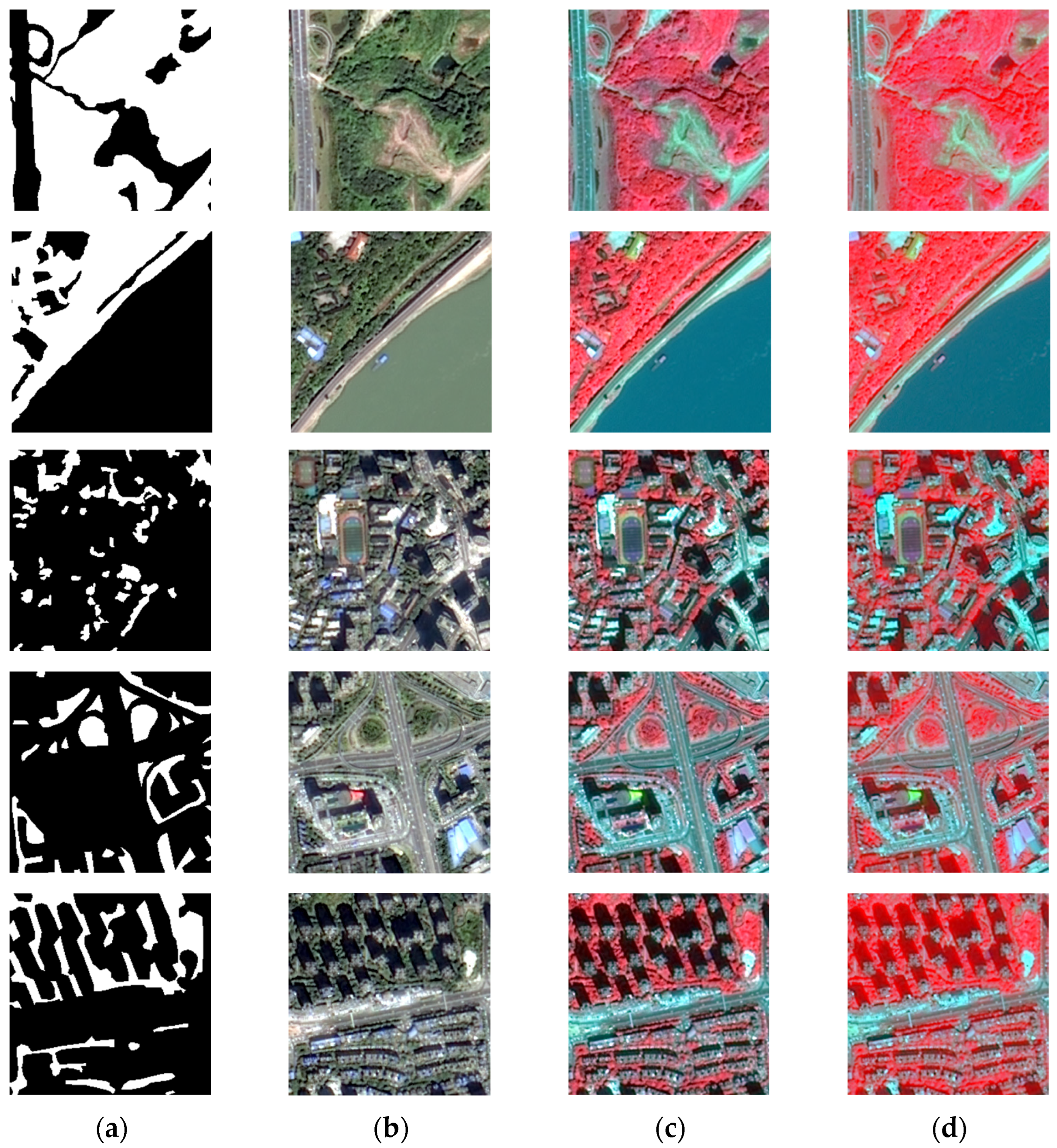
| Images |  |  |  |  |  |  |
| Labels |  |  |  |  |  |  |
| SegNet |  |  |  |  |  |  |
| U-Net |  |  |  |  |  |  |
| SD-UNet |  |  |  |  |  |  |
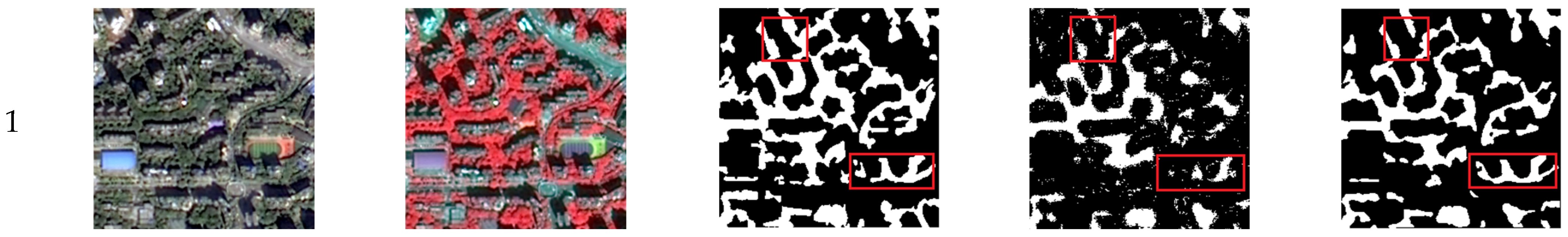
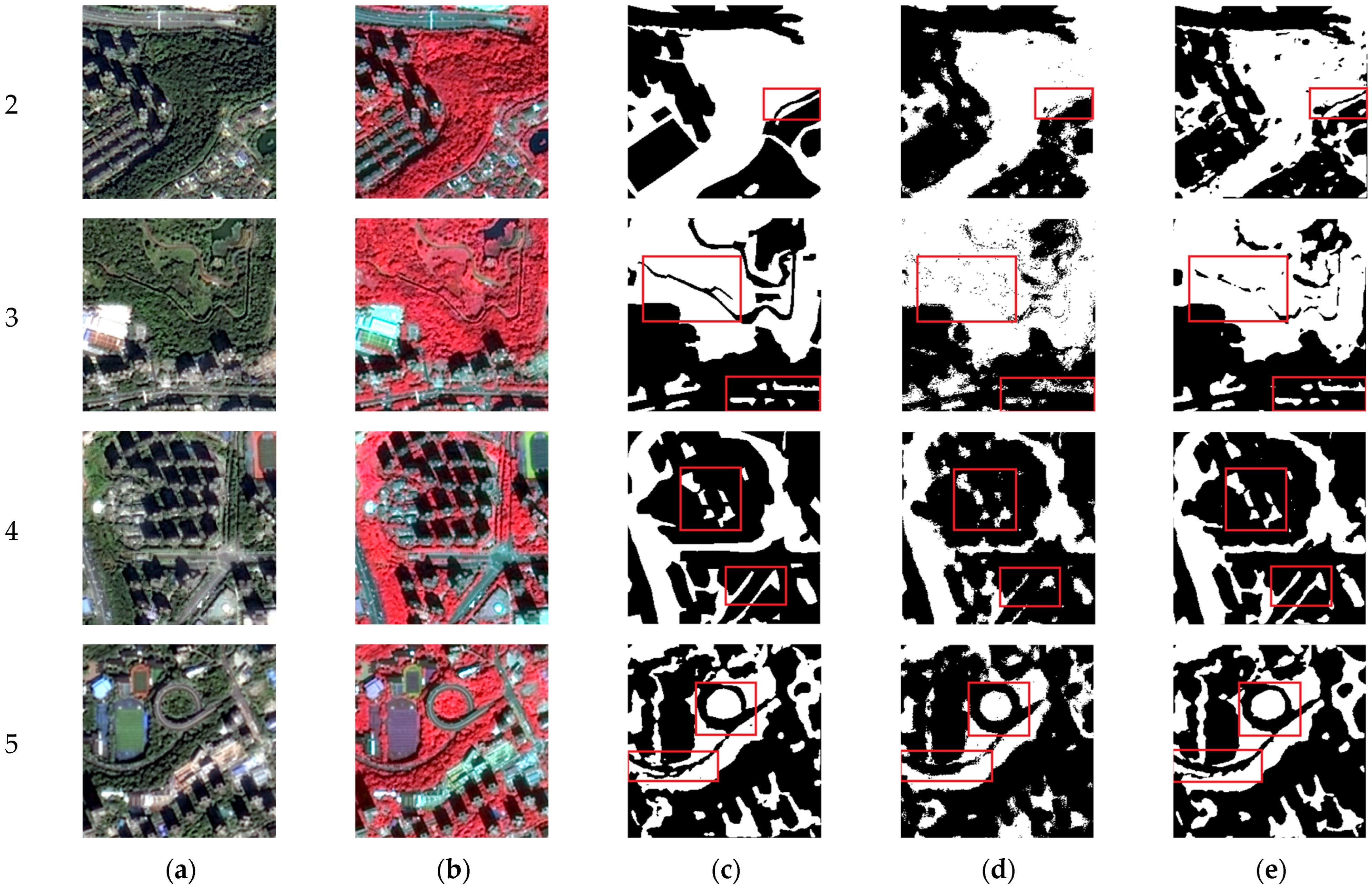
| Note: The red areas of the images represent the vegetation. The colorful boxes in Block 1 and Block 2 represent the marked areas, the white pixels represent the vegetation, and the black pixels represent the background. | ||||||
| Method | Fake Sample Set | NDVI Sample Set | True Sample Set | ||||||
|---|---|---|---|---|---|---|---|---|---|
| ACC | IOU | Recall | ACC | IOU | Recall | ACC | IOU | Recall | |
| SegNet | 0.8902 | 0.7962 | 0.8895 | 0.8910 | 0.5659 | 0.8910 | 0.8673 | 0.5544 | 0.8568 |
| U-Net | 0.9432 | 0.7703 | 0.9419 | 0.9429 | 0.7658 | 0.9422 | 0.9182 | 0.8305 | 0.9163 |
| SD-UNet | 0.9581 | 0.8977 | 0.9577 | 0.9577 | 0.8942 | 0.9572 | 0.9447 | 0.8740 | 0.9442 |
| Method | ACC | IOU | Recall |
|---|---|---|---|
| NDVI | 0.8312 | 0.5996 | 0.8124 |
| RF | 0.8903 | 0.6553 | 0.8734 |
| The best model | 0.9581 | 0.8977 | 0.9577 |
| Scenes | Fake Sample Set | NDVI Sample Set | True Sample Set | |||||||||
|---|---|---|---|---|---|---|---|---|---|---|---|---|
| Clouds and Misty | Building | Suburb | Park | Clouds and Misty | Building | Suburb | Park | Clouds and Misty | Building | Suburb | Park | |
| OA | 0.9256 | 0.9301 | 0.9214 | 0.9392 | 0.9085 | 0.9210 | 0.8605 | 0.9286 | 0.8238 | 0.8821 | 0.8817 | 0.8823 |
| KAPPA | 0.8631 | 0.8750 | 0.8832 | 0.8893 | 0.8055 | 0.8574 | 0.8102 | 0.8565 | 0.6589 | 0.7635 | 0.8325 | 0.7645 |
Disclaimer/Publisher’s Note: The statements, opinions and data contained in all publications are solely those of the individual author(s) and contributor(s) and not of MDPI and/or the editor(s). MDPI and/or the editor(s) disclaim responsibility for any injury to people or property resulting from any ideas, methods, instructions or products referred to in the content. |
© 2023 by the authors. Licensee MDPI, Basel, Switzerland. This article is an open access article distributed under the terms and conditions of the Creative Commons Attribution (CC BY) license (https://creativecommons.org/licenses/by/4.0/).
Share and Cite
Lin, N.; Quan, H.; He, J.; Li, S.; Xiao, M.; Wang, B.; Chen, T.; Dai, X.; Pan, J.; Li, N. Urban Vegetation Extraction from High-Resolution Remote Sensing Imagery on SD-UNet and Vegetation Spectral Features. Remote Sens. 2023, 15, 4488. https://doi.org/10.3390/rs15184488
Lin N, Quan H, He J, Li S, Xiao M, Wang B, Chen T, Dai X, Pan J, Li N. Urban Vegetation Extraction from High-Resolution Remote Sensing Imagery on SD-UNet and Vegetation Spectral Features. Remote Sensing. 2023; 15(18):4488. https://doi.org/10.3390/rs15184488
Chicago/Turabian StyleLin, Na, Hailin Quan, Jing He, Shuangtao Li, Maochi Xiao, Bin Wang, Tao Chen, Xiaoai Dai, Jianping Pan, and Nanjie Li. 2023. "Urban Vegetation Extraction from High-Resolution Remote Sensing Imagery on SD-UNet and Vegetation Spectral Features" Remote Sensing 15, no. 18: 4488. https://doi.org/10.3390/rs15184488