Article

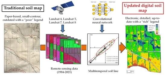
Updating of the Archival Large-Scale Soil Map Based on the Multitemporal Spectral Characteristics of the Bare Soil Surface Landsat Scenes

by
Dmitry I. Rukhovich
1,
Polina V. Koroleva
1,*,
Alexey D. Rukhovich
1 and
Mikhail A. Komissarov
2
1
V.V. Dokuchaev Soil Science Institute, Pyzhevskiy Pereulok 7, 119017 Moscow, Russia
2
Ufa Institute of Biology UFRC RAS, Pr. Oktyabrya 69, 450054 Ufa, Russia
*
Author to whom correspondence should be addressed.
Remote Sens. 2023, 15(18), 4491; https://doi.org/10.3390/rs15184491
Submission received: 28 July 2023 / Revised: 8 September 2023 / Accepted: 11 September 2023 / Published: 12 September 2023
(This article belongs to the Special Issue Remote Sensing for Soil Mapping and Monitoring)

Abstract

:
For most of the arable land in Russia (132–137 million ha), the dominant and accurate soil information is stored in the form of map archives on paper without coordinate reference. The last traditional soil map(s) (TSM, TSMs) were created over 30 years ago. Traditional and/or archival soil map(s) (ASM, ASMs) are outdated in terms of storage formats, dates, and methods of production. The technology of constructing a multitemporal soil line (MSL) makes it possible to update ASMs and TSMs based on the processing of big remote-sensing data (RSD). To construct an MSL, the spectral characteristics of the bare soil surface (BSS) are used. The BSS on RSD is distinguished within the framework of the conceptual apparatus of the spectral neighborhood of the soil line. The filtering of big RSD is based on deep machine learning. In the course of the work, a vector georeferenced version of the ASM and an updated soil map were created based on the coefficient “C” of the MSL. The maps were verified based on field surveys (76 soil pits). The updated map is called the map of soil interpretation of the coefficient “C” (SIC “C”). The SIC “C” map has a more detailed legend compared to the ASM (7 sections/chapters instead of 5), greater accuracy (smaller errors of the first and second kind), and potential suitability for calculating soil organic matter/carbon (SOM/SOC) reserves (soil types/areals in the SIC “C” map are statistically significant are divided according to the thickness of the organomineral horizon and the content of SOM in the plowed layer). When updating, a systematic underestimation of the numbers of contours and areas of soils with manifestations of negative/degradation soil processes (slitization and erosion) on the TSM was established. In the process of updating, all three shortcomings of the ASMs/TSMs (archaic storage, dates, and methods of creation) were eliminated. The SIC “C” map is digital (thematic raster), modern, and created based on big data processing methods. For the first time, the actualization of the soil map was carried out based on the MSL characteristics (coefficient “C”).

Graphical Abstract

1. Introduction

One way to describe the spatial heterogeneity of agricultural lands is soil cartography [1,2]. Soil maps of large scales (1:10,000, 1:25,000) can divide an arable field into several fragments/contours. Each contour of a large-scale soil map contains, as a rule, information on the content of organic matter, the thickness of the humus–accumulative horizon, particle size distribution, acidity, and so on; such properties are usually different from adjacent contours. Without soil maps, it is difficult to implement the concept of landscape-adaptive agriculture [3]. Large-scale soil maps obtained by traditional ground surveys are currently the most widely used [4,5]. Conventional large-scale soil maps (including those processed into vector format) were created, as a rule, more than 30 years ago [6] and need to be updated [7]. Some studies show that in agricultural mapping, soil maps contribute more to the quality of modeling than remote-sensing data (RSD) [8,9].
Monitoring of the soil cover in Russia on a large scale was carried out by two organizations—the agrochemical service [10] and GIPROZEM (State Design Institute of Land Management), which was disbanded in the 1990s during the collapse of the USSR [11]. Large-scale soil maps were compiled by GIPROZEM according to a single instruction for all agricultural lands of the USSR [4]. Four rounds/stages of soil survey took place. Each subsequent round updated the previously made maps. The last one is dated 1980–1992. The arable lands of Russia (RSFSR) under the USSR amounted to 137 million ha and were fully provided with soil maps at a scale of 1: 10,000 or 1: 25,000. Digital soil cartography was not used at that time. At present, the soil maps of the USSR are becoming outdated both in terms of the dates of their compilation and in terms of the obsolescence of the methods for their creation. There is a task of updating archival soil maps (ASM, ASMs).
If the need to update large-scale ASMs is beyond doubt, then different materials and methods for obtaining relevant soil information are offered: traditional ground/field investigations [4], modeling [12,13,14,15] based on the processing of digital elevation models (DEMs) [16,17,18,19,20,21] and climate data [22,23], processing of RSD. Most researchers tend to use the RSD. Several researchers use RSD in the form of vegetation indices (VI, VIs—in the plural) [6,9,24,25,26,27,28,29]. Others use the bare soil surface (BSS) characteristics [7,8,11,30,31,32,33,34,35,36,37]. Still others use ground-based spectroscopy [38].
Both VIs and BSS can use both individual frames of the RSD [39,40,41,42,43,44] and multitemporal series [24,41,45,46,47,48,49]. Multitemporal RSD series are increasingly being used in various areas of economic activity (restoration after fires, snowmelt monitoring, forest dynamics, tundra classification, environmental vulnerability, etc.) [50,51,52,53,54]. When using multitemporal series, traditional VIs are changed by more complex models—LSMM [55] or PARAFAC [49].
Various methods of soil mapping have their own advantages and disadvantages. Ground methods are the most reliable, but also the most time-consuming [4,56]. Modeling gives not real, but potential characteristics of the soil cover [11]. VIs are the most developed and widely applicable but provide only indirect information about the soil cover. Possibly, more promising are the methods of RSD with BSS analysis [7,8,11,30,31,32,33,34,35,36,37].
Detection of BSS from RSD is often practiced based on VIs thresholds [8,36,37]. The frequency of VI application for identifying BSS on RSD shows that for particular tasks (for example, within a single agricultural field), this method can provide acceptable accuracy. Investigations of the BSS location in the RED-NIR spectral space showed that the selection of the BSS by VIs thresholds for the entire Landsat scene gives large errors [34]. At any VI threshold, along with the BSS, areas covered with crop residues, etc. will be detected on the Landsat scene. The authors tend to take a different approach in selecting BSS. Elicitation of BSS is possible on RSD in the spectral neighborhood of the soil line (SNSL) paradigm. The SNSL theory itself is described in a series of articles from 2016–2018 [31,32,33,34,35]. It should be noted that RSD has now taken the form of big data [57]. Processing of big satellite data/RSD is possible both in manual mode (retrospective monitoring of soil and land cover) [58,59,60,61,62] and automated, based on deep machine learning [29,63,64,65,66]. During manual processing, each RSD frame is viewed by the operator for diagnostics and selection of monitoring objects. With an automated technique, the monitoring objects are recognized on each frame of RSD by a neural network, i.e., the operator does not view multitemporal series of RSD. The SNSL theory assumes the possibility of revealing the spatial heterogeneity of the soil cover based on big RSD, but without the use of indicator botany (e.g., VI).
Over decades the archives of RSD have taken the form of big data, and the problem of selecting RSD when forming multitemporal series arises. The selection can be done manually [58,59,60,61,62], algorithmically [8,36,37], or based on artificial intelligence (AI) [9,29,30,63,64,65,66,67]. AI is used as computer vision, but it helps to implement data mining and MapReduce procedures [67,68]. RSD fragments selected by neural network filtering or other methods are used to mapping of intrafield heterogeneity of soil and land cover: ExactFarming [69], FarmersEdge [70], Cropio [71], Intterra [72], AGRO-SAT [73], NEXT farming [74], Agronote [75], OneSoil [76]. Areas of degraded soils are one of the components of the intrafield heterogeneity of the soil cover [24]. The promise of deep machine learning [77] is confirmed by its successful application in various fields: precision agriculture [78,79], medical image diagnostics [80,81], geosensing [82,83], and autonomous driving [84].
When processing RSD for crop production and soil mapping, the RED and NIR channels/bands are most often used [25,26,27,28,85,86]. The use of the RED and NIR channels goes back to the description of the “tasseled cap” [87,88]. At the same time, the development of VIs construction allows the use of other spectral bands in addition to RED-NIR. For example, when calculating EVI, the BLUE channel is used [89]. When calculating LAI, the SWIR channel [90,91] or the GREEN channel is added to the calculations. It is proposed to use the SWIR2 channel for soil cover diagnostic as well [8].
In 2023, the authors checked the correctness of the choice of the RED and NIR spectral bands for the detection of soil degradation according to the BSS [92]. The information content of six Landsat spectral bands for soil mapping (BLUE, GREEN, RED, NIR, SWIR1, and SWIR2) was compared over 37 years [92].
The authors have developed several methods for processing multitemporal RSD series for soil mapping purposes [7,24,29,93]: a method of averaging VIs values, a method of frequency filtering VIs values, and a method of calculating soil line parameters. In the work of 2021 [7], it was suggested that the use of multitemporal BSS series on RSD is highly effective for correcting ASMs and constructing an updated soil map. The work itself was devoted to updating soil maps based on VIs.
In the present work, we intend to test two new approaches to processing RSD that have not previously been used to construct and correct soil maps, in particular:
  • Apply a new method for obtaining the spectral characteristics of BSS based on a multitemporal soil line (MSL).
  • Carry out the selection of multitemporal data of the BSS to build the MSL based on a neural network.
This research aims to test the possibility of updating (correcting) archival large-scale (1:10,000, 1:25,000) soil maps based on the multitemporal spectral characteristics of RED and NIR for BSS conditions with neural network filtering of RSD archives.

2. Materials and Methods

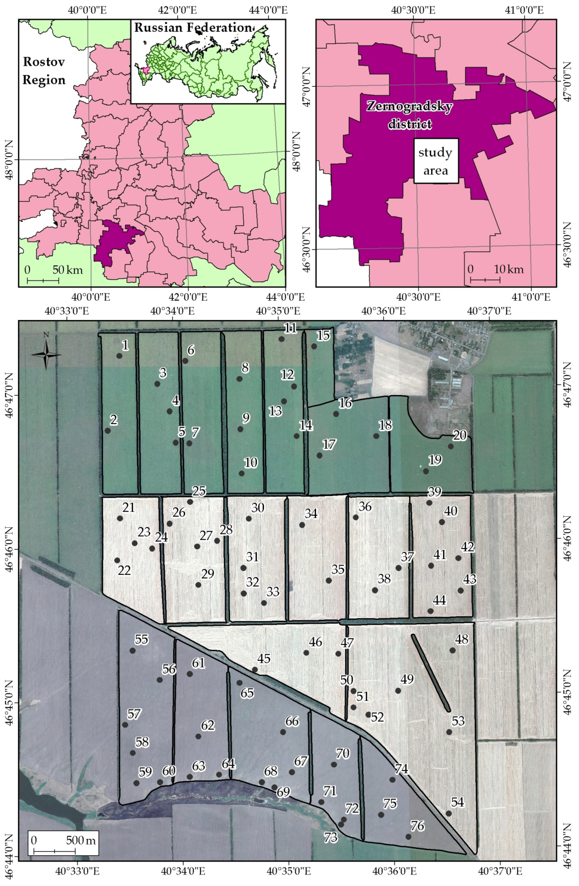
2.1. Study Site Description

The research was carried out on the territory of an agricultural farm with an area of 2215 ha in the Zernogradsky District of the Rostov Oblast (Figure 1). The elevation in the studied site ranged from 50 to 100 m a.s.l. The dominant soils are ordinary chernozems (Haplic Chernozem), medium-thick, carbonate, low-humus, clayey on loess-like clays. The average annual air temperature is 9.3 °C, the sum of active air temperatures (above 10 °C)—3000–3350 °C, and the average annual precipitation—486 mm. The climate of the study area is characterized as temperate continental with mild winters and hot summers or as hot-summer humid continental (Dfa) according to the Köppen climate classification [94]. The Rostov Oblast is an important agricultural region (it produces ~4.6% of all crop and livestock products, or 2nd place within the Russian regions). A high degree of agricultural development (85% of the region’s territory) and frequent land cultivation leads to intensification of various negative/degradation soil processes. Slitization [95,96] and erosion [97] have become widespread. The average soil loss caused by water erosion is 0.83–2.64 mm/yr (6.9–22.0 t ha–1/yr) for arable lands, and deflation rates can reach 55–126 t ha–1/yr [98].

2.2. Methods

2.2.1. A Group of Methods for Creating Vector Versions of Large-Scale Soil Maps

Storage. There is no public repository of large-scale soil maps in electronic form in Russia. Maps are stored in the territorial divisions of Rosreestr [99] in paper form. The maps are cut into fragments of A4 or A3 formats, which are pasted on a gauze base. The maps are stacked up and stored in folders of A4 and A3 formats. The folders contain the names of collective/state farms of the USSR, the name of the administrative district, and the subject of the RSFSR (Union Republic of the former USSR, currently the Russian Federation).
Search. There are no schemes of borders and names of collective/state farms of the RSFSR in the public domain and Rosreestr’s storage facilities. Geographic coordinates were not plotted on large-scale soil maps. There are two methods for searching soil information for a given territory: (1) accurate to the region (i.e., start georeferencing all soil maps of the region), (2) view all maps of the region one by one and search for the names of rivers and settlements.
Scanning. The soil map on a paper-gauze carrier has a large thickness (3–5 mm) and large dimensions (more than 3 × 5 m). For scanning, wide-format scanners with adjustable widths of scanned materials are used.
Gluing. Neighboring fragments A4 and A3 of large-scale soil maps may not be geographically neighbors with an accuracy of about 5 mm (sometimes up to 1 cm of paper). Given the scale of the map, this can be 50 m in nature. This is due to cutting fragments of cards and sticking fragments on gauze. In this regard, after scanning, it is necessary to separate each fragment of A3 or A4 into separate images. Then these fragments need to be assembled into a spatially internally correct raster image.
Georeferencing. Since there are no geographic coordinates on paper large-scale soil maps, they are georeferenced to topographic maps at a scale of 1:25,000 or RSD with a spatial resolution of about 1 m. One raster image is georeferenced to another. For georeferencing, the most clearly identifiable objects of both maps are used—rivers, roads, settlements, etc. (in most cases, soil maps did not have triangulation points).
Vectorization. After accurate georeferencing of large-scale soil maps, manual or semi-automatic [100] vectorization of exclusively soil information is carried out. Legends of these maps are used as a database for the vector version of soil maps.
As a result of six consecutive actions, the most geographically accurate vector version/form of a large-scale soil map is obtained.

2.2.2. A Group of Methods for Obtaining Multitemporal Spectral Characteristics of BSS

Choice of Sources

To construct a multitemporal series of RSD spectral characteristics, several circumstances must be met:
(1)
Long-term period of data acquisition;
(2)
The unity in frequency of receiving frames (scenes);
(3)
Unity of spatial resolution;
(4)
Sufficiency of spatial resolution for solving the task;
(5)
Unity of spectral characteristics;
(6)
Unity of spectral correction methods.
All conditions are currently met by the archives of RSD Landsat 4, 5, 7, 8, 9: the archives cover the period from 1984 to the present (2023), six spectral imaging ranges of bands (BLUE, GREEN, RED, NIR, SWIR1, and SWIR2) are the same for all 5 spacecraft, the spatial resolution of 30 m is the same for six spectral channels, a single atmospheric correction is applied.

Filtering of RSD Frames Unsuitable for BSS Calculations

To calculate the coefficients of the MSL [35], it is necessary to have an open soil surface/BSS on the RSD frames. To do this, is required to select RSD frames or fragments of RSD frames where there would be no vegetation, clouds, water, soot, crop residues, snow, etc. The selection of suitable images can be done manually on the principles of SNSL. The result of manual selection can be converted into a dataset. Based on the dataset, it is possible to carry out machine learning and automate the filtering of RSD. This problem was solved by the authors based on the development and application of gradient boosting and a neural network [29].

Application of Machine Learning for Filtering RSD (Gradient Boosting and Neural Network)

A good machine-learning method for filtering suitable RSD is gradient boosting [101]. The implementation of the method is described in detail by Rukhovich et al. [29]. The manually created dataset was applied. The dataset contains a set of RSD fragments indicating vegetation, cloudiness, waterlogging, snow, and so on. The CatBoost [102] library of the Python programming language for machine learning using the gradient boosting method was used. The logistic function is used as the default loss function for a binary classification problem. For two classes with labels y ∈ {0.1} and predicted probability p, the loss Formula (1) is:
L o g L o s s y , p = y l o g p 1 y l o g 1 p
The classifier is trained for 200 iterations with a learning rate of 0.01. Because the collected dataset is highly unbalanced, we set unequal weights for both classes; more specifically, their values are 0.01 and 0.99. Strong imbalance means the ratio of detected (recognizable) objects in the dataset to the rest data in which the array is less than 1/100. It is worth noting that with a strong sample imbalance, the specified training accuracy of 95% can be achieved without detecting (recognizing) any object.
To train the neural network, the same dataset was used for gradient boosting. The task is similar to the gradient boosting procedure—binary classification of the image—“suitable” and “not suitable”. Training methodology is described in detail in the work of 2021 [29]. The standard architecture of the convolutional neural network for the binary classification problem is used. Such architectures typically [103,104] consist of a pair of convolutional blocks followed by a pooling layer and another pair of fully connected layers. In turn, the convolutional block contains a convolutional layer, a normalization layer, an activation layer, and a maximal pooling layer. Input layer shape 128 × 128 × 8; here 8 channels include: RED, GREEN, BLUE, NIR, SWIR1, SWIR2, NDVI, and binary field mask.

Recognition of BSS

For the full scene of the RSD (Landsat, Sentinel), the BSS in the RED-NIR spectral plane takes the form of an ellipse [34]. The authors believe that the BSS in the spectral space of RED and NIR takes the form of an ellipse. The ellipse of the BSS spectral characteristics is located on the soil line between the zones of crop residues (straw) and traces of agricultural fires (soot) [34]. In this regard, the BSS on the entire RSD frame cannot be distinguished based on VIs [34,105]. The ellipse of the spectral BSS values can be manually selected on the “tasseled cap” graphs [87,88]. It is possible to form a dataset from manually selected BSS areas on RSD for 37 years. Based on the dataset, it is possible to carry out machine learning and automate the filtering of RSD. This problem was solved by the authors based on the development and application of a neural network [93].

The Use of a Neural Network in the Recognition of BSS

The creation and application of a neural network for BSS recognition is described in detail in 2022 [93]. The method consists of training a neural network based on a dataset. The dataset is a series of Landsat scenes for the period from 1984 to 2021 in which the BSS is distinguished. The theory of SNSL was used to identify the BSS contours. According to this theory, BSS occupies a specific place on the “tasseled cap” plot. The SNSL location only partially coincides with the soil line for NDVI-type VIs [106]. The trained neural network makes it possible to identify BSS on any Landsat frames in similar soil and climatic conditions.
Deep machine learning uses the popular neural architecture for image segmentation U-Net [83], the ReLU activation function and batch normalization [107], the Dice loss function [108], and the Adam optimization algorithm [109].

Machine-Learning Quality Assessment

(1)
Test selection/sample. A set of objects not used in training;
(2)
Acceptance selection/sample. A set of objects not used in elaboration;
(3)
Sliding control (cross-validation, CV) [110,111]. The training sample is divided into N parts and training is performed N times on N (1 part, without repetitions).

Calculation of the Average Multitemporal Characteristics of the BSS

The authors showed that a “tasseled cap” can be built not only for an RSD frame but also for each RSD pixel based on the totality of the received spectral values of RED and NIR for 30 or more years on the same type of RSD [34] (Figure 2a). As a result, an MSL can be constructed [34,112] (Figure 2). Since the BSS multitemporal characteristics also take the form of an ellipse, it is proposed to use the ellipse parameters of the multitemporal spectral values for calculating the single BSS multitemporal characteristics of each pixel. In the present study, the remoteness of the center of the ellipse from the origin of the spectral plane RED and NIR—the coefficient “C” is used as a multitemporal characteristic of the BSS [34] (Figure 2b). In terms of describing the multitemporal spectral distribution of the BSS characteristics, the coefficient “C” is some kind of average long-term spectral value of RED-NIR in each pixel. The physical meaning of the coefficient “C” is also mentioned in Section 4.1.
A map of the BSS spectral characteristics can be constructed for areas of the earth’s surface where the BSS occurs quite often. In our studies, such areas are arable land. Forest belts, roads, settlements, etc. are removed from the calculations, and information about the arable boundaries was obtained by retrospective monitoring of the soil and land cover.

2.2.3. Retrospective Monitoring of Soil and Land Cover

The method is described in a series of works in 2013–2020 [58,59,60,61,62]. The method makes it possible to restore the change in the arable land’s boundaries in the period from the present to 1968. Special detailing is carried out from 1984 to the present when there was a high dynamic of plowing areas in Russia [113]. The method is based on the interpretation of satellite imagery of different spatial resolutions: high (IKONOS, GeoEye-1, WorldView, etc.) [114] and medium spatial resolution (Landsat, Sentinel) [115], as well as archival data of 1968 and 1975 (CORONA) [116]. The accuracy of the method corresponds to that of conventional mapping at a scale of 1:10,000 [117,118]. The method requires a GIS project of a certain composition and quality.

2.2.4. Ground Verification Methods

To assess the quality of conventional ASMs and soil maps built on the principles of SNSL, it is necessary to conduct a traditional field soil survey. A field survey requires determining the places for laying soil profiles, which according to the method [4], take into account the relief and RSD. In modern conditions, this requires the creation of a GIS project.

Creation of a GIS Project

A GIS project should include the following georeferenced information: topographic maps, aerial photography, DEM, and updated RSD of high and medium resolution.

Creation of a Ground Survey Plan

Based on the GIS of the project, the coordinates of the soil pits (cross-section/profiles) locations are determined. The soil pits should characterize slopes, watersheds, thalwegs, depressions, etc. In the case of a large-scale survey, soil pits can be laid based on the density—one pit per 15–50 ha of arable land.

Ground Data Collection

The soil profile is excavated to a depth of 0.5–1.5 m, usually to the illuvial horizon (B) or parent rock (C). For each profile, a soil description, photographing, and sampling are carried out. The coordinates of the soil pits are recorded by a GPS receiver. A soil sample is taken from the top 0–10 cm layer of each cross-section to measure the organic matter (OM) content. The thickness of the humus (also known as humus–accumulative or organomineral) horizon was also measured. The thickness of the humus horizon was understood as the total thickness of the A and AB horizons [119,120,121]. The content of OM was determined according to the Tyurin method [122]. A direct analog of Tyurin’s method for determining OM is the method of Walkley-Black [123].
When describing the soil profiles and using the values of the OM content in the plow layer and the thickness of the humus horizon, the type and subtype of soil and the presence of degradation were determined. Degradation was understood as a decrease in the thickness of the humus horizon and/or a decrease in the content of OM in the plow layer in relation to the typical A+AB depth and humus content of the soil for the study region.

2.2.5. Cartographic Analysis

Cartographic analysis was carried out in ArcGIS [124]. All materials are collected in this GIS shell. The main method of analysis was the pairwise intersection of different GIS layers of the project. The results of the intersection were recorded in spreadsheets. In spreadsheets, the quantitative parameters of the obtained combinations were evaluated, and regression equations were constructed.

2.2.6. Atmospheric Correction

For Landsat and Sentinel, the atmospheric correction was carried out using the ATCOR module of the ERDAS Imagine software package [125].

2.2.7. Estimating the Accuracy of Soil Maps

The assessment of accuracy was carried out in terms of information theory: errors of the first kind (type I error, false-positive result) and errors of the second kind (type II error, false negative result). In the present work, this means:
(1)
False-positive result—the contour of the soil map included soil cross-sections with the name of soils that do not match the name in this contour according to the map legend;
(2)
False negative result—cross-sections with soil names identical to the legend are outside the contour.

2.2.8. Flowchart of Research

Figure 3 shows a flowchart of the application and grouping of the 20 methods used in the current investigation. The methods are grouped into two large blocks. The first block is the work with traditional soil maps (TSMs), both with the paper and vector versions on a large scale. The second block is the processing of big RSD stored in the cloud. The methods of the second block make it possible to obtain a soil map based on the processing of the multitemporal spectral characteristics of the BSS. The second block can be implemented by more traditional methods of selecting big data manually and according to specified criteria, or by more modern methods using machine learning. The flowchart shows at what stages of work the machine learning was used.
The results of both blocks are verified based on traditional ground observations/survey methods and compared with each other.
The final result of the work of both blocks is an updated digital soil map.

3. Results

3.1. GIS Project (Used Materials)

A GIS project was created for the territory of the Zernogradsky district, Rostov Oblast, including the following layers:
(1)
Topographic maps at a scale of 1:25,000 and 1:50,000;
(2)
Panchromatic aerial photography of 2012 with a spatial resolution of 0.6 m (orthophotomap);
(3)
Digital elevation model (SRTM) 1 arcsecond [21];
(4)
Scanned analog space imagery of 1968 with a spatial resolution of 1.8 m (panchromatic, KH-4B satellite, US CORONA mission);
(5)
Scanned analog space imagery of 1975 with a spatial resolution of 6 m (panchromatic, KH-9 satellite, US CORONA mission);
(6)
RSD Landsat 4–8 from 1985 to 2022;
(7)
Space imagery Sentinel-2 2016–2022.

3.2. Ground Surveys

Based on the GIS project, a ground survey was carried out in April of 2022. A total of 76 soil profiles were laid. The location of the soil pits is shown in Figure 1. The measurement results are summarized in Table 1. There are 7 soil varieties described/detected of the following soil types/subtypes:
(1)
Chernozem-meadow, slitized, compacted, thick—high thickness of humus horizon, low-humus, clayey on hypergenized loess-like clays (chernozem-meadow slitized);
(2)
Meadow–chernozem, deeply slitized, compacted, thick, low-humus, clayey on hypergenized loess-like clays (meadow-chernozem deeply slitized);
(3)
Meadow-chernozem, thick, low-humus, clayey on loess-like clays (meadow-chernozem);
(4)
Ordinary chernozem, medium-thick, carbonate, low-humus, clayey on loess-like clays (ordinary chernozems);
(5)
Ordinary chernozem, medium-thick, slightly eroded, carbonate, slightly humus, clayey on loess-like clays (ordinary chernozem slightly eroded);
(6)
Ordinary chernozem, thin, moderately eroded, carbonate, slightly humus, clayey on loess-like clays (ordinary chernozem moderately eroded);
(7)
Ordinary chernozem, thin, strongly eroded, carbonate, slightly humus, clayey on loess-like clays (ordinary chernozem strongly eroded).
Table 1. Characteristics of the soil.
No. of Soil Pit Soil Name Number under the Field Description (Table 2)SOM Content (0–10 cm, %)Thickness of Organic Horizons (A + AB, cm)Soil Name Number According to the TSM (Table 3)Coefficient “C” ValuesSoil Name/Number on the SIC “C” Map (Table 2)
144.66620.1503164
214.79310.1408342
344.97130.1483054
4634030.1625056
514.48010.1402222
644.57520.1521824
714.28010.1394641
834.88520.1479333
914.79010.1398071
1053.25030.1561625
1144.57420.1517324
1244.78120.1513514
1353.35320.1558325
1424.29920.1402522
1514.58820.1353041
1634.68320.1465233
1724.98920.1402692
1835.39020.1449513
1944.67820.1518664
20359620.1446253
2114.78230.1369061
2244.97530.1468553
2344.26130.1500514
24545730.1494834
2514.69130.1353321
26457530.1481914
2743.96130.1556745
2834.18730.1415602
2944.26330.1521164
3024.37710.1413482
3153.75430.1517444
3253.75730.1549355
3344.56030.1522034
3424.28730.1384591
3543.77130.1513314
3644.86130.1518514
3724.29230.1365191
3843.96430.1508884
3915.28110.1387361
40545530.1522024
4124.18530.1424062
4253.85630.1544245
4344.37730.1463853
4454.35930.1500744
4553.95330.1520834
4663.64930.1540315
4753.95430.153235
4844.56530.1506454
4943.66130.1538335
5043.96630.1539275
5172.93230.1662877
5263.24530.1608686
5353.55430.1552225
5453.65240.1546995
5544.86340.1497334
5653.65340.1530595
5762.94250.1621816
5844.77950.1470113
5973.13650.1644037
6072.92950.1714837
6153.65140.1577365
62634340.1625006
6372.72250.1809387
6472.62250.1803187
6535.29240.1461793
6653.65140.1547925
6763.24540.1594946
6872.73050.1782287
69733350.1701667
7063.14340.1567115
7172.72840.1641937
7263.14040.1615616
7343.76040.1555705
7463.14240.1575945
7544.16940.1507094
7653.55540.1549085
The average OM content of the ordinary chernozem was 4.5%, and the thickness of the organomineral layer was 75 cm, which is in good agreement with the characteristics of this zonal soil—ordinary chernozem, medium-thick, carbonate, low-humus, clayey on loess-like clays [119,120]. This soil type is characterized by the following values—the thickness of the humus horizon is 60–80 cm and the OM content is 4–6% [126,127]. Threshold values for the OM content and the thickness of the humus horizon (4% and 60 cm); below such values the soil is considered subject to degradation.
Soil pits are added to the GIS project as a point layer.

3.3. Scheme of Arable Land

Based on the GIS project, a retrospective monitoring of the soil and land cover was carried out. The boundaries of 20 agricultural fields were digitized with a scale accuracy of 1:10,000. The area of digitization was 2215 ha (Figure 1).

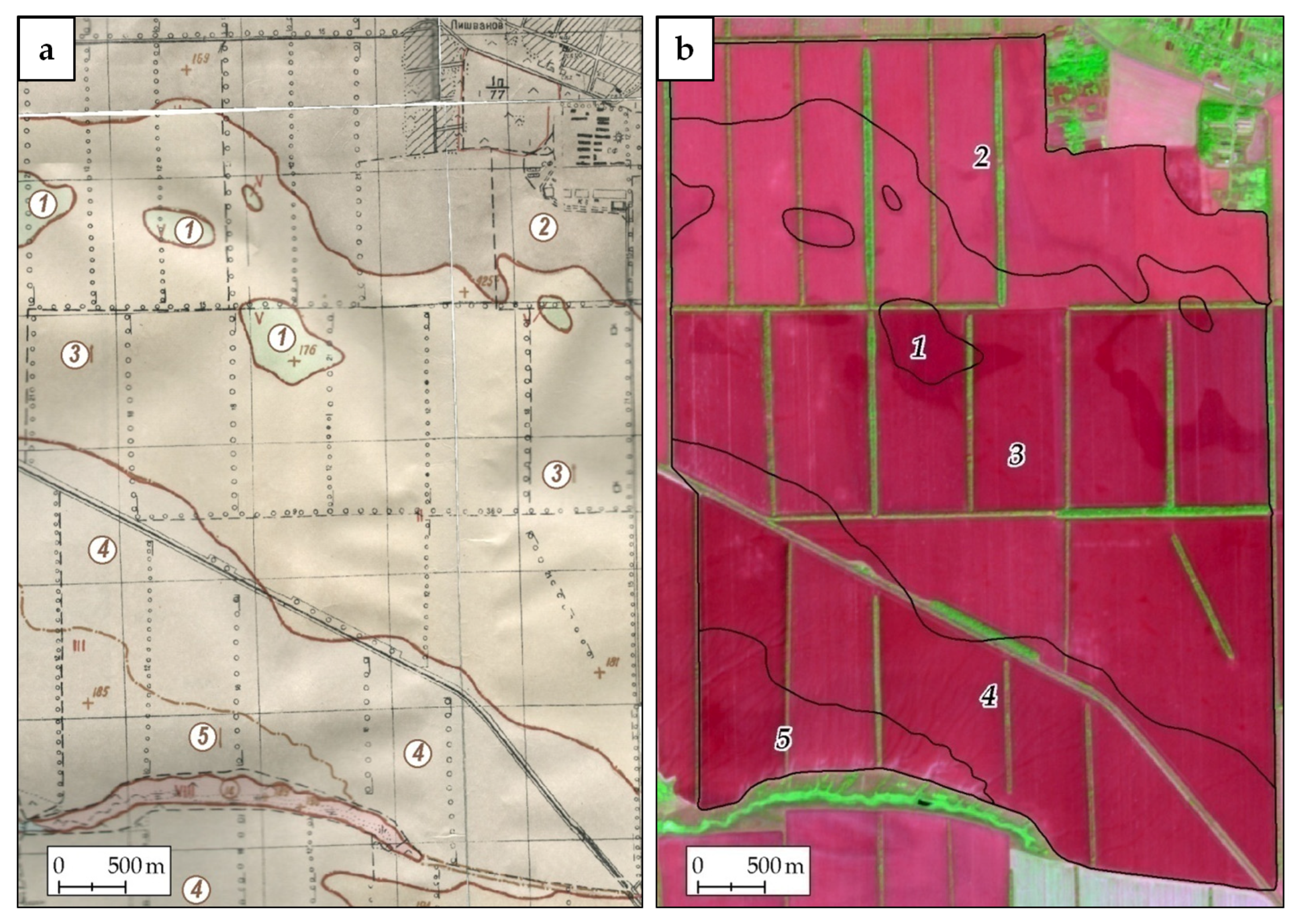
3.4. Vector Version of a Traditional Soil Map (TSM)

The result of georeferencing of a TSM in raster form is shown in Figure 4a. The vector version of the TSM was obtained for all arable lands of the study area. The map consists of 9 contours (Figure 4b).

3.5. Selection of Frames Suitable for Calculations of RSD and Detection of BSS

Based on machine learning, 244 Landsat frames for the period from 1984 to 2021 were selected from 1028 in the archives. Based on the neural network on the selected 244 frames, the areas of the BSS were identified.

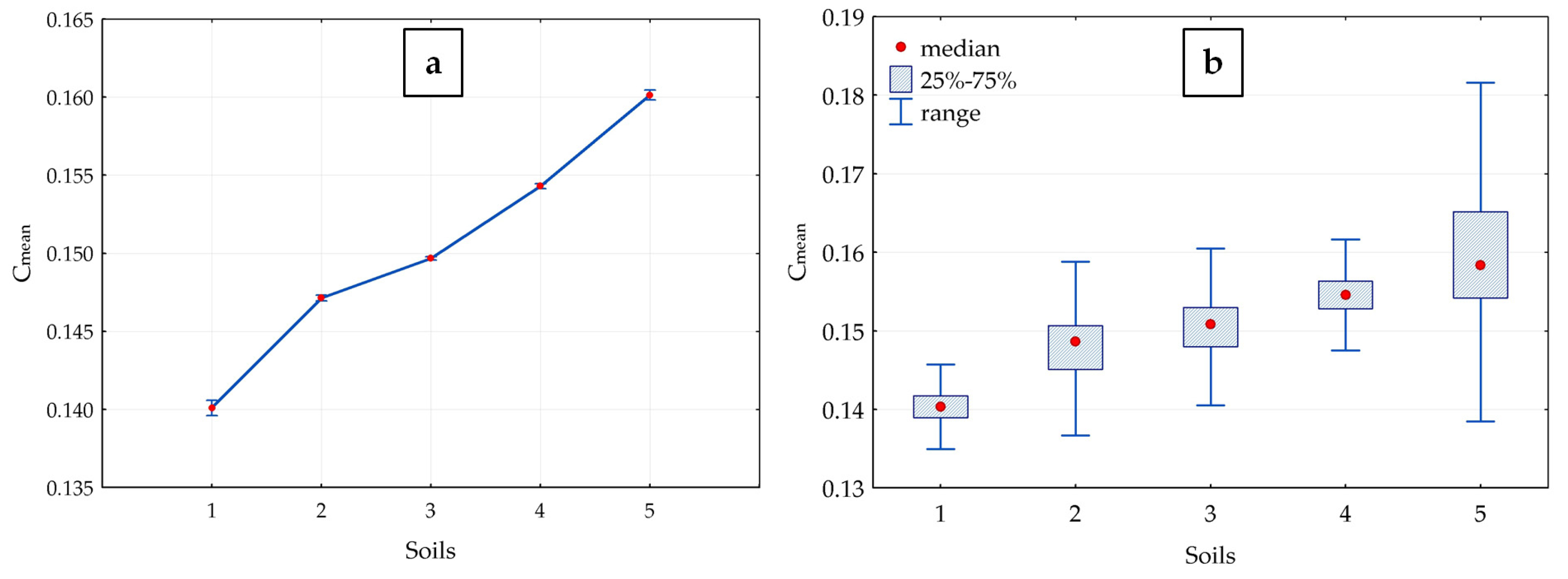
3.6. Map of Values of Coefficient “C” of Multitemporal Soil Line (MSL)

For each of the 24,611 pixels for the studied territory, the parameters of the ellipse approximation of the MSL were calculated. A map with the coefficient “C” values of the MSL is shown in Figure 5a. The coefficient “C” values for each of the 76 soil pits are given in Table 1.

3.7. Intersection of the TSM and the “C” Coefficient Map

The intersection of the vector version of a TSM and the map of coefficient “C” values was carried out. Each soil type/variation in the TSM was assigned average values of the coefficient “C” for the certain soil type (Figure 5b).
Figure 5b shows a map of the average “C” coefficient values for each legend class in the TSM. For the convenience of analysis, the coloring of the resulting map is similar to the map of coefficient “C” values. It follows from Figure 5 that all classes of the legend in the TSM have their average values of the “C” coefficient, which differ from each other. The average values of the “C” coefficient for each class of the legend in the TSM are statistically significantly different (Table S1 and Figure 6a). This confirms both the information content of the multitemporal spectral characteristics for soil cover detection and the quality of the TSM.
In other words, the values of the “C” coefficient have a soil interpretation, and the soil contours of a TSM have their own spectral characteristics.

3.8. Map of Soil Interpretation of Coefficient “C” (SIC “C”)

Based on the intersection of the soil cross-section map and the map of the coefficient “C”, the ranges of coefficient “C” values characterizing each of the 7 soil varieties were selected (Table 2). A map of the soil interpretation of the “C” coefficient was constructed (Figure 7).
The cartographic materials obtained during the work were added as additional separate layers to the GIS project (the first 7 layers are shown in Section 3.1):
(8)
Map of soil profiles;
(9)
Scheme of arable land;
(10)
Raster georeferenced TSM;
(11)
Vector georeferenced TSM;
(12)
Map of coefficient “C”.

3.9. Analysis

3.9.1. Correction of the TSM Based on the Results of Intersection of the TSM and the Map of “C” Coefficient Values

The results of the intersection of the TSM and the map of the “C” coefficient values look more complicated if we present not only the average values, but also the characteristics of the ranges of the “C” coefficient values (Figure 6b) for soil-type differences. It follows from the graph that the ranges of coefficient “C” values for different classes of the legend in the TSM significantly overlap. Thus, the ranges of spectral values of meadow soils are entirely within the ranges of values for ordinary chernozems. The range of coefficient “C” values of chernozem slightly eroded generally includes all ranges of other soil varieties. This makes it difficult to correctly determine the ranges of the “C” coefficient for soil interpretation of the spectral values.
On the other hand, the very existence of a map of the average values of the “C” coefficient for each class of the legend of the TSM (Figure 4) indicates the possibility of setting the ranges of the “C” coefficient values for soil interpretation. Possible ranges of the coefficient “C” values for the legend of the TSM are presented in Table 3.

3.9.2. Comparison of the TSM and the Soil Interpretation Map of the “C” Coefficient

Figure 8 shows a map of the soil interpretation of the coefficient “C” with the contour boundaries of the TSM superimposed on it. For the convenience of analysis, the SIC “C” map is presented in a coloring similar to the coloring of the “C” coefficient map in Figure 5a.
First, it should be noted that the SIC “C” map has a richer legend of 7 points. On the TSM, there are no overcompacted slitized soils and soils with medium and strong erosion levels. Detection of overcompacted slitized soils is important for agriculture because these areas are lower in fertility than zonal soil. Also, the moderate and severe level of erosion is negatively affected on soil fertility. For the needs of modern precision farming, the TSM is depleted of information on negative/degradation soil processes.
Second, it is necessary to note the omissions of contours on the TSM. So, the soils of the meadow group/row are marked on the TSM on 5 contours. These contours on the SIC “C” map correspond to overcompacted slitized soils. On the SIC “C” map, there are twice as many contours of overcompacted slitized soils as there are soils of the meadow series on the TSM (Figure 7 and Figure 8). The areas of distribution of overcompacted slitized soils are five times larger on the SIC “C” map than on the TSM (Table 2 and Table 3).
The TSM, in comparison with the SIC “C” map, significantly underestimates the soil nomenclature and the areas of distribution of soil types and subtypes with the manifestation of degradation processes (Table 2 and Table 3).

3.9.3. Estimation of the TSM Accuracy Based on the Results of Ground Surveys

The TSM contains 5 soil names (Table 3). During field survey/verification (76 soil profiles are analyzed), 7 soil names were identified (Table 2). The conformity between the soil names of the TSM and the names of soils according to the field survey is shown in Table 4. Table 4 gives the numbers of soils taking into account Table 3, and shows how many soil profiles with names according to Table 2 fell within the soil contours of the TSM.
According to Table 4 on the TSM there is no moderately and severely degraded soil on arable land. In the contours of deflated soils, only 41% of soil pits with degradation are noted. Compacted slitized soils are marked as soils of the meadow series. It is difficult to assess the accuracy of a TSM in terms of information theory for all 5 soil types. It is much easier to pass to the concept of false-positive results if we group the legend of the TSM into 3 groups: meadow soils, non-degraded chernozems, and degraded chernozems. Soils according to data from field survey (soil profiles description) can be grouped similarly:
(1)
Soils of the meadow series.
In total, soils of the meadow series are described in 14 (soil pits) out of 76 possible. Of these, 6 fell into the meadow soil contours in the TSM (Class 1, Table 3). No other soil pits were noted in the contours of meadow soils. The errors of the first kind for soils of the meadow series were 0%, and the errors of the second kind were 57%. Thus, most of the meadow soils are located outside the meadow contours in the TSM. The contours themselves are defined correctly.
(2)
Non-degraded chernozems.
Non-degraded chernozems should make up 100% of soils in the contours of Class 2 (Table 3) and 75–90% in Class 4. Class 2 is provided by 13 soil pits, 9 of which are non-degraded chernozems. In total, non-degraded chernozems are found in 29 of the soil sample points. Error of the first kind—31%, 55%—of the second. Similar to the soils of the meadow series, non-degraded chernozems in most cases are located outside the contours of non-degraded soils in the TSM. The contours of non-degraded soils themselves are well distinguished, but they include soils of the meadow series.
(3)
Non-degraded chernozems in combination with degraded chernozems.
Class 4 (Table 3) contains 15 soil profiles. Based on the legend of the TSM, 4 of them should refer to degraded chernozems and 11 to non-degraded ones (20% to 80%). According to the field survey, 12 soil profiles were classified as degraded, and 3 as non-degraded. An error of the first kind—53%. The contours of Class 4 (Table 3) are poorly distinguished because they underestimate the spread of a degradation process—erosion.
(4)
Deflated chernozems.
The contours of deflated chernozems (Class 3, Table 3) contain 34 soil pits, of which 14 belong to degraded soils. An error of the first kind is 59%. The contours of Class 3 (Table 3) are poorly distinguished because significantly overestimate the distribution of degraded soils. The contours should be attributed to non-degraded soils in combination with degraded soils. Also, in the contours, there is a large distribution of soils of the meadow series.
(5)
Degraded chernozems.
Slightly eroded soils have Class 5 (Table 3). For this Class, 8 soil pits are detected/described, of which 6 are highly degraded soils and one soil profile/point is moderately degraded soil. The error of the first kind is 12.5%. The contours of Class 5 are generally correct. The main disadvantage of these contours is the legend. According to this legend, Class 5 is poorly eroded soil. According to a field survey, these soils are predominantly strongly eroded.
An error of the second kind was calculated for all contours of degraded soils (Classes 3, 4, and 5; Table 3) and amounted to 35%. The entire area of erosion distribution is identified better than Classes 3 and 4, which are included in this area.
As we can see, even with the coarsening of the legend, only the contours of meadow slitized and strongly eroded soils have an acceptable error of the first kind, 0 and 12.5%. The error of the second kind is large for all contours of the TSM without exception. This means that the TSM underestimates the distribution of meadow slitized overcompacted soils, and moderately and strongly eroded soils. The remaining soils in more than 50% of cases are situated outside their contours. For all contours of the map, 37 out of 76 soil profiles can be attributed to being in their classes.

3.9.4. Assessment of the SIC “C” Map Accuracy Based on the Results of Ground Surveys

Since the legend of the SIC “C” map was created based on a field survey, the soil naming classes of the map and soil profiles are identical. Only combinations of soil profiles and contours of the map should be considered (Table 5).
(1)
Class 1 (Table 2)—chernozem-meadow soils. The first kind of error (type I error) is 25%, and the second (type II error)—14%. Errors summed up only because of the mutual intersection of Class 1 and Class 2—meadow-chernozem soil. The soils are spectrally and morphologically similar. The main difference is the degree of soil moisture. Both soils are slitized and overcompacted.
(2)
Class 2 (Table 2)—meadow-chernozem soils. Error of I and II types are the same—33%. Errors are totalized due to the joint intersection of Class 2 with Classes 1 and 3—meadow-chernozem soil. The soils are spectrally and morphologically similar. The main difference is the degree of moisture and the degree of compaction, as well as the slitization factor. If the intersection of Classes 1 and 2 can be considered to be a minor error, Class 3 refers to non-degraded chernozems with a higher degree of moisture supply, i.e., Classes 1 and 2 refer to soils with low agricultural productivity, and Class 3 to high ones.
(3)
Class 3 (Table 2)—meadow-like chernozem soils. Type I error is 33% and type II error is 14%. Errors are added up due to the mutual intersection of Class 3 with Class 2—meadow–chernozem soil.
(4)
Class 4 (Table 2)—ordinary chernozems, not degraded. Type I error is 24% and type II error is 27%. Most of the errors (9 out of 11) are added up due to the mutual intersection of Class 4 and Class 5—ordinary chernozem slightly eroded. The soils are spectrally and morphologically similar. The main difference is the thickness of the humus horizon and the OM content in the arable layer. The identification of these soils, even in the field, is not always possible.
(5)
Class 5 (Table 2)—ordinary chernozem slightly eroded. Type I error is 39% and type II error is 31%. Errors are added up due to the mutual intersection of Class 5 with classes—4 and 6—ordinary chernozem moderately eroded. The distinguishing of chernozem according to the degree of erosion is possible only according to the humus horizon thickness and the OM content in the plow horizon. In space, this is a very smooth transition, which is difficult to detect spectrally.
(6)
Class 6 (Table 2)—ordinary chernozem moderately eroded. Type I error is 0% and type II error is 33%. Errors are formed due to the mutual intersection of Class 6 with Class 5—ordinary chernozem slightly eroded.
(7)
Class 7 (Table 2)—ordinary chernozem strongly eroded. Type I and II errors are the same—0%. The spectral brightness of strongly eroded soils increases sharply because humus horizons are almost completely lost. Low-humus carbonate horizons with high reflectivity come to the surface.
For the reasons and magnitudes of type I and II errors, Classes 2 and 5 can be distinguished as the most problematic. These classes intersect with two adjacent classes. This shows the smoothness of spatial transitions in the meadow series of soils (chernozem-meadow and meadow-chernozem) and in the series of increasing degrees of erosion from non-degraded to moderately degraded.
Across the entire SIC “C” map, 56 out of 76 soil profiles fell into their classes.

3.9.5. Comparison in the Accuracy of the TSM and the SIC “C” Map When Both Maps Are Aggregated into Three Classes

As already noted, the TSM and the SIC “S” map have different legends with a different number of classes. Using Table 5, both maps can be reclassified into a single legend:
(1)
Consider meadow-chernozem soils on hypergenized clays (Class 1, Table 3) and slitized soils (Classes 1 and 2, Table 2) as synonyms. It is conditionally possible to call this association the soils of the meadow series.
(2)
Consider ordinary chernozems (Class 2, Table 3) and non-degraded soils (Classes 3 and 4, Table 2) as synonyms. It is conditionally possible to call this association non-degraded chernozems.
(3)
Consider as a single class the entire area of eroded soils (Classes 3, 4, 5; Table 3) and Classes 5, 6, and 7 of Table 2. Conventionally, this association can be called eroded soils.
With this combination, one can compare the accuracy of both maps in general terms of information theory:
Soils of the meadow series of the TSM: errors of the first kind 0%, errors of the second kind 57%. Soils of the meadow series of the SIC “C” map: errors of the first kind 7%, errors of the second kind 0%.
Chernozems non-degraded of the TSM: errors of the first kind 30%, errors of the second kind 55%. Non-degraded chernozems of the SIC “C” map: errors of the first kind 18%, errors of the second kind 18%.
Eroded soils of the TSM: errors of the first kind 53%, errors of the second kind 35%. Eroded soils of the SIC “C” map: errors of the first kind 12.5%, errors of the second kind 15%.
Thus, the accuracy of the SIC “C” map is approximately three times higher than the accuracy of the TSM.

3.9.6. Characteristics of the TSM by Organic Matter (OM)

The OM content was measured in 76 soil profiles (Table 1). The graph (Figure 9) shows the average values and confidence intervals of the average OM content by classes of the TSM legend. The graph shows a clearly expressed trend of a decrease in the OM content from non-eroded chernozems to eroded soils. It should be noted that, according to Tukey’s criterion (Table S2), none of their soil varieties differ significantly from all the others.
A similar graph (Figure 10) shows the dependence of the organomineral horizon thickness on the class of the TSM legend. There is also a well-observed tendency to decrease the thickness of the humus horizon according to the degree of erosion manifestation. According to Tukey’s criterion, none of their soil varieties differs significantly from all the others (Table S3).

3.9.7. Characteristics of the SIC “C” Map in Terms of OM

Figure 11 shows a graph of average OM content values for 7 soil classes of the SIC “C” map. The downward trend in the OM content can be traced for Classes 3–7, i.e., for the following series of soils: meadow-chernozem, ordinary chernozem, slightly eroded, moderately eroded, and strongly eroded. In this series, only moderately and strongly eroded soils are not statistically significant (Table S4). Under plowing conditions, the OM content of strongly and moderately eroded soils does not depend on the degree of erosion.
Slitized and meadow soils stand apart. The slitized soils are statistically indistinguishable from meadow-chernozem soils and ordinary chernozem in terms of OM content. Obviously, on slitized soils, with an increase in moisture, there is no OM content increase. Most likely, this is due to their lower productivity, and consequently a lower delivery of plant residues.
According to the humus horizon thickness, five groups of soils differ significantly: the group of soils of the meadow series (Classes 1–3, Table 2) and four soils in terms of the degree of erosion (Figure 12 and Table S5). Soils of the meadow series stand apart, as well as in terms of the OM content. It should be noted that the thickness of organomineral horizons in meadow soils is greater than in zonal soils, but this humus layer does not increase with an increase in meadowness level.

3.9.8. Possibility of Interpretation of Soil Maps as Maps of OM Stocks

Soil maps can serve as a basis for estimating and mapping soil carbon stocks as part of a national carbon balance inventory, as well as provide baseline data for monitoring climate change impacts and informing land management decisions [128,129,130,131].
Stocks of OM depend on the humus horizon thickness and the OM content. Judging by the graphs (Figure 9, Figure 10, Figure 11 and Figure 12), both maps can be interpreted as maps of the OM content, since each contour has its own certain values of the humus horizon thickness and the OM content in the plow horizon. The accuracy of estimating OM reserves is better for the SIC “C” map because the map is more subdivided (the range of values for soil classes of humus layer thickness and OM content is larger) and sections of the legend in more cases are statistically significantly separated by both indicators.

4. Discussion

4.1. Physical Interpretation of Investigations

This study was carried out as part of testing several hypotheses: the existence of an MSL [34], the information content of the SNSL [93], the uniqueness of the MSL coefficients [35], and the possibility of soil interpretation of the MSL coefficients. It was assumed that the spectral brightness of the BSS varies in different periods for each pixel of the RSD according to unique patterns. Soil moisture is assumed to be the main factor that changes the brightness of a pixel. The wetter the soil—the lower the reflectivity. The second factor is agricultural practices (plowing, harrowing, sowing, etc.). In principle, the loosening of the soil also primarily affects the brightness of the BSS through moisture. When loosening, wetter layers come to the surface, which reduces the reflectivity.
If over time the soil brightness depends on their moisture, then in the soil space aspect—the OM content in the upper horizons influences the reflectivity. The higher the OM content—the lower the soil reflectivity. The third factor is the soil texture. As a rule, when sandy fractions dominated in the particle size distribution, then the soil has a greater reflectivity in comparison with fine-textured (prevalence of clay and/or silt) soil [132,133].
Thus, wet soil with a high OM content will be darker than dry soil with a lower OM content with the same particle size distribution. However, dry soil with more OM can be darker than wet soil with less OM content. That is why it is difficult, if at all possible, to separate soils based on spectral brightness in a single image. The situation is complicated by the presence of vegetation/crop rotations when only a part of the soil is BSS.
During the growing season, BSS goes through all stages of moisture. In addition, it happens repeatedly. The spectral brightness of the BSS over many years forms an ellipse of possible BSS values. The ellipse is described by the coordinates of the center in the RED-NIR spectral plane, the angle of inclination of the major axis, and the length of the major and minor axes. The minimum brightness values in the ellipse correspond to the wettest soil conditions in the pixel. The maximum values correspond to the driest soil condition in the pixel. In general, dry and wet periods mutually compensate for the brightness values, and the coordinates of the center of the ellipse become characteristic of the average pixel brightness values [34].
In this case, soils with a high OM content will have the center coordinates of the ellipse closer to the center of the RED-NIR spectral plane, and those with less OM further. For meadow soils, the moisture factor will be of great importance, i.e., wetter soils of depressions (meadow soils) will be located closer to the center of the plane than zonal soils on watersheds.
By constructing MSL for each pixel for 35 years, it is possible to calculate the distance of the ellipse center from the origin of the RED-NIR spectral plane—the value of the “C” coefficient.
In the study area, the values of the coefficient “C” increased in the following row of soils:
  • Chernozem-meadow, slitized, compacted, thick, low-humus, clayey on hypergenized loess-like clays (chernozem-meadow slitized);
  • Meadow-chernozem, deeply slitized, compacted, thick, low-humus, clayey on hypergenized loess-like clays (meadow-chernozem deeply slitized);
  • Meadow-chernozem, thick, low-humus, clayey on loess-like clays (meadow-chernozem);
  • Ordinary chernozem, medium-thick, carbonate, low-humus, clayey on loess-like clays (ordinary chernozems);
  • Ordinary chernozem, medium-thick, slightly eroded, carbonate, slightly humus, clayey on loess-like clays (ordinary chernozem slightly eroded);
  • Ordinary chernozem, thin, moderately eroded, carbonate, slightly humus, clayey on loess-like clays (ordinary chernozem moderately eroded);
  • Ordinary chernozem, thin, strongly eroded, carbonate, slightly humus, clayey on loess-like clays (ordinary chernozem strongly eroded).
In the same row, the OM content, the thickness of the humus horizon, and moisture are decreased.
The hypothesis of the information content of the MSL coefficients was confirmed when the TSM was updated. The number of types and subtypes of soils that are displayed on the map has increased, the accuracy of mapping contour boundaries has increased, and the correspondence of the map to the names of soils defined in the field has improved.
Increased reflectivity is also an indicator of non-compliance with the rules of soil use/management, which leads to an increase in soil losses due to erosion and, as a result, a decrease in the content of SOM [134].
This is the physical interpretation of the work; the need for this interpretation is substantiated in [135]. As a physical interpretation, regression models of calculated indicators from field measurements were used [136,137].

4.2. Description of Soil Maps

The TSM has completely understandable construction logic. This logic is based on relief analysis (Figure 13). The lower part of the slope belongs to eroded soils (Class 5, Table 3). The middle part of the slope belongs to the complex of eroded and non-eroded soils (Class 4, Table 3). The most elevated part is deflated soils (Class 3, Table 3). Flat surfaces are occupied by zonal soils—ordinary chernozems (Class 2, Table 3). Local depressions are identified as meadow-chernozem soils (Class 1, Table 3). In the study area on the TSM, 5 soil profiles are plotted, confirming the logic of construction. It should be noted that no soil profiles were laid in the areas of strongly eroded soils.
The accuracy of the TSM is described above. It is worth noting that 76 soil pits showed a significantly greater soil diversity in the study area than the TSM. Thus, the identification of soil contours based on the relief of the considered territory does not describe a more complex picture of the real soil cover spatial heterogeneity.
The SIC “S” map (Figure 6) also looks logical and does not contradict the topography. The spectral characteristics confirm that the lower part of the slope with southern exposure is occupied by eroded soils. Spectral characteristics make it possible to divide erosion lands into strong and medium. In addition, meadow–chernozem soils were detected on the SIC “C” map within the slope (Figure 8), confirmed by ground surveys (Figure 6, soil sample points 58 and 65). The SIC “C” map showed that the heterogeneity of the slope allows ordinary chernozem, meadow-chernozem, and chernozem-meadow soils to exist locally within these slope limits.
The presence of water erosion on the upper slope part is also confirmed. However, the spectral characteristics make it possible to operate not only by the ratio of eroded and non-eroded soils but also by separating these soils in space. The percentage of slightly eroded soils is significantly higher than on the TSM.
The location of the contour of weakly deflated soils in the watershed, identified on the TSM, could not be confirmed by ground surveys and spectrally. In reality, the watershed surface is occupied by ordinary chernozems and meadow soils. Degraded soils occupy a smaller part of the watershed.
Ordinary chernozems non-degraded occupy most of the watershed. In the area of ordinary chernozems, ground-based studies, and spectral characteristics detect many slitized meadow soils.
The soils of the meadow series are indeed located in relief depressions. The drawdown values (relative depth) are about one meter with a total height difference of 50 m over the study area. Such height differences are poorly detected on the DEM SRTM. The spectral characteristics make it possible to clearly define the boundaries of the distribution of the meadow series and slitized soils.
Thus, both maps show the applicability of the paradigms within which they were created. The paradigm of applying the MSL characteristics showed the possibility of a more accurate display of the soil cover on the SIC “C” map compared to the TSM created in the paradigm of the dominance of the relief factor.

4.3. Review of Similar Studies

The possibility of using the characteristics of the BSS on RSD for detecting the spatial heterogeneity of soil and land covers is, in principle, not denied. On the other hand, for the analysis of RSD, VI is most often used. Even on the topic (Special Issue) with an explicit indication of the BSS “Remote Sensing for Cropping Systems and Bare Soils Monitoring and Optimization”, in most works a VIs were used [25,26,27,28,85,86]. There is a change of crops: corn [26], durum wheat [27], rice [28], and wheat [25], but the methods of processing RSD change little. NDVI predominates, and LAI is sometimes supplemented by other VIs.
The authors observe VI as an indirect method for revealing the spatial heterogeneity of the soil and land cover. VIs are a kind of indicator botany, when the state of vegetation determines the heterogeneity of the Earth’s surface. The transition from indirect signs to the measurement of multitemporal brightness, as shown by this work, makes it possible to identify 7 soil differences.
The following are articles on the current Special Issue—“Remote Sensing for Soil Mapping and Monitoring”:
(1)
The process of isolating BSS on RSD.
In a series of papers, we have shown that the BSS on RSD occupies an elliptical area in the RED-NIR spectral space. This area is on the same line from the center of coordinates with the areas of crop residues, waterlogging, and places of agricultural fires. The NDVI threshold defines a sector from the origin in the RED-NIR spectral plane. Cloudiness also partially falls into this sector. Using NDVI thresholds, it is impossible to single out the BSS without capturing three or four adjacent spectral areas. At the same time, in several studies, BSS was distinguished precisely by the NDVI thresholds [8,36,37]. It remains to be assumed that the colleagues do not have problems with the detection of areas with crop residues, clouds, fires, and waterlogging.
(2)
Application of VIs.
Of the seven works [6,8,9,30,36,37,38], three used VI [6,9,30]. In the work of 2021 [7], we showed that it is possible to apply VI to correct soil maps, but this is not enough. The poor condition of crops can be due to various soil reasons. In the present study, as in the work of 2021, areas of low fertility are associated with waterlogging and erosion, which look the same in VI. It remains to be assumed that colleagues in the work meet territories with only one characteristic of the soil cover that affects the state of vegetative crops.
(3)
Informativeness of soil data.
In two works [8,9], a conclusion is made about a greater contribution to the quality of soil information modeling compared to RSD. At the same time, soil information is, as it were, a third-party component. In this case, the question remains: “where can one really obtain actual large-scale information on the soil cover?” Ground methods are known to be very time-consuming and expensive. The present study is precisely aimed at obtaining updated large-scale soil information based on RSD. We assume this information/approach will be useful to colleagues and improve the model quality.
(4)
Multitemporal series.
In several works [30,37,45,53], the application of multitemporal RSD series in the topic of agriculture and landscape classification is studied, which brings together the directions of our research. Of particular interest is the approach of applying multitemporal series of RSD with the use of the BSS spectral characteristics [37,45]. In other areas of knowledge, multitemporal series are used more widely [46,47,48,49,50,51,52,53,54]. We believe that the use of a multitemporal series of BSS spectral characteristics opens up great prospects for studying the spatial heterogeneity of agricultural landscapes.
(5)
Correction of soil maps.
Consonant with this study are studies on the correction of ASM [6]. The use of previously accumulated knowledge about the structure of the soil cover allows a better understanding of the functioning of agricultural landscapes. The application of the present BSS study does not negate the information content of VI. The synthesis of these methods can give a greater accuracy of work on the creation of updated information on the soil cover.

4.4. Direction for Further Research

The works [31,34] show the very possibility of constructing an MSL. The work of 2022 [93] shows the information content of an MSL for detecting degraded areas on the soil cover. In 2023, Rukhovich et al. [92] showed the correctness of the choice of RED-NIR spectral bands. In the present study, the information content of the coefficient “C” of the MSL for updating the soil map with 7 soil differences is shown. However, in all these studies, Landsat data were used for the maximum period of time—more than 35 years. It is necessary to establish the stability of the proposed method for constructing soil maps to the time interval of the used RSD and the number of RSD frames.
It is necessary to set a balance when the number of RSD frames turns into quality. In other words, when the amount of RSD becomes big data. By “big data” in prospective research, we mean a state of data where it is possible to extract information from the entire data set that cannot be extracted from a smaller data set in principle.
First, it is necessary to study the time intervals while maintaining the source of information (Landsat). If the result of the study is positive, the coefficients of the MSL can be used to monitor the state of the BSS.
The second direction is to study the number of RSD. If the number of RSD dominates over the time interval, prospects for using RSD spectrally similar to Landsat, but with a smaller time coverage (Sentinel) will open up.

5. Conclusions

This study shows the results of applying two approaches designed to solve all three problems of ASMs/TSMs: updating, converting to a digital vector form, and using big RSD processing methods for updating maps. The approaches/technologies are being demonstrated for the first time. The technologies include several methods for processing a big RSD, which were developed and published by the authors in a series of articles in 2016–2023 [7,11,29,31,32,33,34,35,92,93]. Technologies are combinations of methods, including the determination of the BSS location based on analysis of the RED-NIR spectral space; selection of RSD frames for calculations based on a trained neural network; the BSS identification on the RSD frame based on the trained neural network; construction of an MSL; and retrospective monitoring approach. The technological chain (sequence of actions) is shown in the form of a flowchart. The main novelty of the present work is the demonstration of the possibility of combining contemporary technologies/methods/approaches for processing big RSD for ASM updating. Until now, such technologies have not been provided and statistically substantiated.
The first technology makes it possible to convert the ASM as carefully as possible into a digital vector form with the most accurate georeferencing. In vector form, all the original information from the paper map is stored.
The second technology allows the creation of a soil map of the coefficient “C” of the MSL. For the first time, it was possible to carry out a correction of a large-scale soil map based on the coefficient “C” of MSL. The presence of a relationship between the values of the MSL coefficient “C” and soil-type areals on the TSM is shown. This indicates that the values of the “C” coefficient have a soil interpretation, and the soil contours of the TSM have their own spectral characteristics. Based on the coefficient “C” map, it was possible to update large-scale soil information. The actualization of TSM is solved in the form of a map based on soil interpretation of the coefficient “C” (SIC “C”). The map of coefficient “C” was obtained completely automatically, i.e., for the first time, the correction of the ASM was carried out without the participation of an operator in the processing of big RSD.
The SIC “C” map (updated soil map) has a more detailed legend than the TSM (7 positions against 5) and three times greater accuracy. The accuracy of the maps was defined in terms of information theory: errors of the first kind (false positive) and errors of the second kind (false negative). The updated map retains continuity with the ASM. One of the advantages of the updated map is its suitability for calculating stocks of soil organic matter/carbon (SOM/SOC). The suitability lies in the fact that the contours of the updated soil map differ statistically significantly from each other in terms of the thickness of humus-accumulative horizons and the SOM content in the arable layer. The second advantage is a more accurate localization of places with the manifestation of negative/degradation soil processes (slitization, strong and moderate erosion).
For the first time, the correction of a large-scale soil map led to an increase in accuracy not only in terms of more quality mapping of soil contours/boundaries but also in increasing the number of soil contours and in expanding the map legend (areas with new soil subtypes could be detected) while maintaining a given map scale.

Supplementary Materials

The following supporting information can be downloaded at: https://www.mdpi.com/article/10.3390/rs15184491/s1, Table S1: Post hoc analysis of the means of Cmean values in soils of traditional soil map (significant differences are shown in red); Table S2: Post hoc analysis of the means of OM content in soils of traditional soil map (significant differences are shown in red); Table S3: Post hoc analysis of the means of thickness of humus horizon in soils of traditional soil map (significant differences are shown in red); Table S4: Post hoc analysis of the means of OM content in soil varieties of SIC “C” map (significant differences are shown in red); Table S5: Post hoc analysis of the means of thickness of humus horizon in soil varieties of SIC “C” map (significant differences are shown in red).

Author Contributions

Conceptualization, D.I.R.; methodology, D.I.R. and P.V.K.; software, A.D.R. and M.A.K.; validation, P.V.K.; formal analysis, A.D.R.; investigation, D.I.R.; data curation, P.V.K.; writing—original draft preparation, D.I.R.; writing—review and editing, M.A.K.; visualization, A.D.R.; project administration, D.I.R. All authors have read and agreed to the published version of the manuscript.

Funding

The research was conducted within the framework of state assignment No. FGUR-2022-0009.

Data Availability Statement

Publicly available Landsat datasets were analyzed in this study. These data can be found here: http://earthexplorer.usgs.gov, accessed on 21 June 2023. The other data that support the findings of this study are available on request from the corresponding author.

Conflicts of Interest

The authors declare no conflict of interest.

References

  1. Fridland, V.M. Structure of the soil mantle. Geoderma 1974, 12, 35–41. [Google Scholar] [CrossRef]
  2. Fridland, V.M. Pattern of the Soil Cover; John Wiley & Sons: Hoboken, NJ, USA, 1977; ISBN 9780470991671. [Google Scholar]
  3. Kiryushin, V.I. The management of soil fertility and productivity of agrocenoses in adaptive-landscape farming systems. Eurasian Soil Sci. 2019, 52, 1137–1145. [Google Scholar] [CrossRef]
  4. Ischenko, T.A. (Ed.) All-Union Instruction on Soil Surveys and the Compilation of Large-Scale Soil Land Use Maps; Kolos: Moscow, Russia, 1973. (In Russian) [Google Scholar]
  5. Web Soil Survey. Available online: https://websoilsurvey.nrcs.usda.gov/app/ (accessed on 1 June 2023).
  6. Jędrejek, A.; Jadczyszyn, J.; Pudełko, R. Increasing accuracy of the soil-agricultural map by Sentinel-2 images analysis—Case study of maize cultivation under drought conditions. Remote Sens. 2023, 15, 1281. [Google Scholar] [CrossRef]
  7. Rukhovich, D.I.; Koroleva, P.V.; Kalinina, N.V.; Vilchevskaya, E.V.; Suleiman, G.A.; Chernousenko, G.I. Detecting degraded arable land on the basis of remote sensing big data analysis. Eurasian Soil Sci. 2021, 54, 161–175. [Google Scholar] [CrossRef]
  8. Zhang, X.; Xue, J.; Chen, S.; Wang, N.; Shi, Z.; Huang, Y.; Zhuo, Z. Digital mapping of soil organic carbon with machine learning in dryland of Northeast and North plain China. Remote Sens. 2022, 14, 2504. [Google Scholar] [CrossRef]
  9. Taghizadeh-Mehrjardi, R.; Emadi, M.; Cherati, A.; Heung, B.; Mosavi, A.; Scholten, T. Bio-inspired hybridization of artificial neural networks: An application for mapping the spatial distribution of soil texture fractions. Remote Sens. 2021, 13, 1025. [Google Scholar] [CrossRef]
  10. Nekrasov, R.V. On the guard of Russian soils fertility. Agrochem. Her. 2019, 52, 1137–1145. (In Russian) [Google Scholar] [CrossRef]
  11. Kulyanitsa, A.L.; Rukhovich, D.I.; Koroleva, P.V.; Vilchevskaya, E.V.; Kalinina, N.V. Analysis of the informativity of big satellite precision-farming data processing for correcting large-scale soil maps. Eurasian Soil Sci. 2020, 53, 1709–1725. [Google Scholar] [CrossRef]
  12. Farifteh, J.; Van Der Meer, F.; Atzberger, C.; Carranza, E.J.M. Quantitative analysis of salt-affected soil reflectance spectra: A comparison of two adaptive methods (PLSR and ANN). Remote Sens. Environ. 2007, 110, 59–78. [Google Scholar] [CrossRef]
  13. Higginbottom, T.P.; Symeonakis, E. Assessing land degradation and desertification using vegetation index data: Current frameworks and future directions. Remote Sens. 2014, 6, 9552–9575. [Google Scholar] [CrossRef]
  14. Ibrahim, Y.Z.; Balzter, H.; Kaduk, J.; Tucker, C.J. Land degradation assessment using residual trend analysis of GIMMS NDVI3g, soil moisture and rainfall in sub-Saharan west Africa from 1982 to 2012. Remote Sens. 2015, 7, 5471–5494. [Google Scholar] [CrossRef]
  15. Mendonça-Santos, M.D.L.; Dart, R.O.; Santos, H.G.; Coelho, M.R.; Berbara, R.L.L.; Lumbreras, J.F. Digital soil mapping of topsoil organic carbon content of Rio de Janeiro state, Brazil. In Digital Soil Mapping; Boettinger, J.L., Howell, D.W., Moore, A.C., Hartemink, A.E., Kienast-Brown, S., Eds.; Springer: New York, NY, USA, 2010; pp. 255–266. [Google Scholar] [CrossRef]
  16. Glazunov, G.P.; Gendugov, V.M. A full-scale model of wind erosion and its verification. Eurasian Soil Sci. 2003, 36, 216–226. [Google Scholar]
  17. Larionov, G.A.; Dobrovol’skaya, N.G.; Krasnov, S.F.; Liu, B.Y. The new equation for the relief factor in statistical models of water erosion. Eurasian Soil Sci. 2003, 36, 1105–1113. [Google Scholar]
  18. Maltsev, K.A.; Yermolaev, O.P. Potential soil loss from erosion on arable lands in the European part of Russia. Eurasian Soil Sci. 2019, 52, 1588–1597. [Google Scholar] [CrossRef]
  19. Sukhanovskii, Y.P. Rainfall erosion model. Eurasian Soil Sci. 2010, 43, 1036–1046. [Google Scholar] [CrossRef]
  20. Shary, P.A.; Sharaya, L.S.; Mitusov, A.V. Fundamental quantitative methods of land surface analysis. Geoderma 2002, 107, 1–32. [Google Scholar] [CrossRef]
  21. SRTM. Available online: http://srtm.csi.cgiar.org (accessed on 1 June 2023).
  22. Romanenkov, V.A.; Smith, J.U.; Smith, P.; Sirotenko, O.D.; Rukhovitch, D.I.; Romanenko, I.A. Soil organic carbon dynamics of croplands in European Russia: Estimates from the “model of humus balance”. Reg. Environ. Change 2007, 7, 93–104. [Google Scholar] [CrossRef]
  23. Rukhovich, D.I.; Koroleva, P.V.; Vilchevskaya, E.V.; Romanenkov, V.A.; Kolesnikova, L.G. Constructing a spatially-resolved database for modelling soil organic carbon stocks of croplands in European Russia. Reg. Environ. Change 2007, 7, 51–61. [Google Scholar] [CrossRef]
  24. Khitrov, N.B.; Rukhovich, D.I.; Koroleva, P.V.; Kalinina, N.V.; Trubnikov, A.V.; Petukhov, D.A.; Kulyanitsa, A.L. A study of the responsiveness of crops to fertilizers by zones of stable intra-field heterogeneity based on big satellite data analysis. Arch. Agron. Soil Sci. 2020, 66, 1963–1975. [Google Scholar] [CrossRef]
  25. Zhang, Y.; Walker, J.P.; Pauwels, V.R.N.; Sadeh, Y. Assimilation of wheat and soil states into the APSIM-wheat crop model: A case study. Remote Sens. 2022, 14, 65. [Google Scholar] [CrossRef]
  26. Qi, G.; Chang, C.; Yang, W.; Gao, P.; Zhao, G. Soil salinity inversion in coastal corn planting areas by the satellite-UAV-ground integration approach. Remote Sens. 2021, 13, 3100. [Google Scholar] [CrossRef]
  27. Romano, E.; Bergonzoli, S.; Pecorella, I.; Bisaglia, C.; De Vita, P. Methodology for the definition of durum wheat yield homogeneous zones by using satellite spectral indices. Remote Sens. 2021, 13, 2036. [Google Scholar] [CrossRef]
  28. Iwahashi, Y.; Ye, R.; Kobayashi, S.; Yagura, K.; Hor, S.; Soben, K.; Homma, K. Quantification of changes in rice production for 2003–2019 with MODIS LAI data in Pursat province, Cambodia. Remote Sens. 2021, 13, 1971. [Google Scholar] [CrossRef]
  29. Rukhovich, D.I.; Koroleva, P.V.; Rukhovich, D.D.; Kalinina, N.V. The use of deep machine learning for the automated selection of remote sensing data for the determination of areas of arable land degradation processes distribution. Remote Sens. 2021, 13, 155. [Google Scholar] [CrossRef]
  30. Zhang, L.; Cai, Y.; Huang, H.; Li, A.; Yang, L.; Zhou, C. A CNN-LSTM model for soil organic carbon content prediction with long time series of MODIS-based phenological variables. Remote Sens. 2022, 14, 4441. [Google Scholar] [CrossRef]
  31. Rukhovich, D.I.; Rukhovich, A.D.; Rukhovich, D.D.; Simakova, M.S.; Kulyanitsa, A.L.; Bryzzhev, A.V.; Koroleva, P.V. The informativeness of coefficients a and b of the soil line for the analysis of remote sensing materials. Eurasian Soil Sci. 2016, 49, 831–845. [Google Scholar] [CrossRef]
  32. Rukhovich, D.I.; Rukhovich, A.D.; Rukhovich, D.D.; Simakova, M.S.; Kulyanitsa, A.L.; Bryzzhev, A.V.; Koroleva, P.V. Maps of averaged spectral deviations from soil lines and their comparison with traditional soil maps. Eurasian Soil Sci. 2016, 49, 739–756. [Google Scholar] [CrossRef]
  33. Kulyanitsa, A.L.; Rukhovich, A.D.; Rukhovich, D.D.; Koroleva, P.V.; Rukhovich, D.I.; Simakova, M.S. The application of the piecewise linear approximation to the spectral neighborhood of soil line for the analysis of the quality of normalization of remote sensing materials. Eurasian Soil Sci. 2017, 50, 387–396. [Google Scholar] [CrossRef]
  34. Koroleva, P.V.; Rukhovich, D.I.; Rukhovich, A.D.; Rukhovich, D.D.; Kulyanitsa, A.L.; Trubnikov, A.V.; Kalinina, N.V.; Simakova, M.S. Location of bare soil surface and soil line on the RED–NIR spectral plane. Eurasian Soil Sci. 2017, 50, 1375–1385. [Google Scholar] [CrossRef]
  35. Koroleva, P.V.; Rukhovich, D.I.; Rukhovich, A.D.; Rukhovich, D.D.; Kulyanitsa, A.L.; Trubnikov, A.V.; Kalinina, N.V.; Simakova, M.S. Characterization of soil types and subtypes in N-dimensional space of multitemporal (empirical) soil line. Eurasian Soil Sci. 2018, 51, 1021–1033. [Google Scholar] [CrossRef]
  36. Karyotis, K.; Tsakiridis, N.L.; Tziolas, N.; Samarinas, N.; Kalopesa, E.; Chatzimisios, P.; Zalidis, G. On-site soil monitoring using photonics-based sensors and historical soil spectral libraries. Remote Sens. 2023, 15, 1624. [Google Scholar] [CrossRef]
  37. Broeg, T.; Blaschek, M.; Seitz, S.; Taghizadeh-Mehrjardi, R.; Zepp, S.; Scholten, T. Transferability of covariates to predict soil organic carbon in cropland soils. Remote Sens. 2023, 15, 876. [Google Scholar] [CrossRef]
  38. Yang, M.; Chen, S.; Guo, X.; Shi, Z.; Zhao, X. Exploring the potential of vis-NIR spectroscopy as a covariate in soil organic matter mapping. Remote Sens. 2023, 15, 1617. [Google Scholar] [CrossRef]
  39. Xu, H.; Hu, X.; Guan, H.; Zhang, B.; Wang, M.; Chen, S.; Chen, M. A remote sensing based method to detect soil erosion in forests. Remote Sens. 2019, 11, 513. [Google Scholar] [CrossRef]
  40. Phinzi, K.; Ngetar, N.S. Mapping soil erosion in a quaternary catchment in Eastern Cape using geographic information system and remote sensing. S. Afr. J. Geomat. 2017, 6, 11. [Google Scholar] [CrossRef]
  41. Eckert, S.; Hüsler, F.; Liniger, H.; Hodel, E. Trend analysis of MODIS NDVI time series for detecting land degradation and regeneration in Mongolia. J. Arid. Environ. 2015, 113, 16–28. [Google Scholar] [CrossRef]
  42. Ayalew, D.A.; Deumlich, D.; Šarapatka, B.; Doktor, D. Quantifying the sensitivity of NDVI-based C factor estimation and potential soil erosion prediction using Spaceborne earth observation data. Remote Sens. 2020, 12, 1136. [Google Scholar] [CrossRef]
  43. De Carvalho, D.F.; Durigon, V.L.; Antunes, M.A.H.; De Almeida, W.S.; Oliveira, P.T.S. Predicting soil erosion using RUSLE and NDVI time series from TM Landsat 5. Pesqui. Agropecuária Bras. 2014, 49, 215–224. [Google Scholar] [CrossRef]
  44. Yengoh, G.T.; Dent, D.; Olsson, L.; Tengberg, A.E.; Tucker, C.J. Limits to the use of NDVI in land degradation assessment. In Use of the Normalized Difference Vegetation Index (NDVI) to Assess Land Degradation at Multiple Scales; Springer Briefs in Environmental Science; Springer: Cham, Switzerland, 2015; pp. 27–30. [Google Scholar] [CrossRef]
  45. Gallo, B.C.; Magalhães, P.S.G.; Demattê, J.A.M.; Cervi, W.R.; Carvalho, J.L.N.; Barbosa, L.C.; Bellinaso, H.; Mello, D.C.d.; Veloso, G.V.; Alves, M.R.; et al. Soil erosion satellite-based estimation in cropland for soil conservation. Remote Sens. 2023, 15, 20. [Google Scholar] [CrossRef]
  46. van der Werff, H.; Ettema, J.; Sampatirao, A.; Hewson, R. How weather affects over time the repeatability of spectral indices used for geological remote sensing. Remote Sens. 2022, 14, 6303. [Google Scholar] [CrossRef]
  47. Ulfa, F.; Orton, T.G.; Dang, Y.P.; Menzies, N.W. Are climate-dependent impacts of soil constraints on crop growth evident in remote-sensing data? Remote Sens. 2022, 14, 5401. [Google Scholar] [CrossRef]
  48. Huang, H.; Huang, J.; Feng, Q.; Liu, J.; Li, X.; Wang, X.; Niu, Q. Developing a dual-stream deep-learning neural network model for improving county-level winter wheat yield estimates in China. Remote Sens. 2022, 14, 5280. [Google Scholar] [CrossRef]
  49. Lopez-Fornieles, E.; Brunel, G.; Devaux, N.; Roger, J.-M.; Taylor, J.; Tisseyre, B. Application of parallel factor analysis (PARAFAC) to the regional characterisation of vineyard blocks using remote sensing time series. Agronomy 2022, 12, 2544. [Google Scholar] [CrossRef]
  50. Hao, B.; Xu, X.; Wu, F.; Tan, L. Long-term effects of fire severity and climatic factors on post-forest-fire vegetation recovery. Forests 2022, 13, 883. [Google Scholar] [CrossRef]
  51. Stendardi, L.; Karlsen, S.R.; Malnes, E.; Nilsen, L.; Tømmervik, H.; Cooper, E.J.; Notarnicola, C. Multi-sensor analysis of snow seasonality and a preliminary assessment of SAR backscatter sensitivity to arctic vegetation: Limits and capabilities. Remote Sens. 2022, 14, 1866. [Google Scholar] [CrossRef]
  52. Hernández-Romero, G.; Álvarez-Martínez, J.M.; Pérez-Silos, I.; Silió-Calzada, A.; Vieites, D.R.; Barquín, J. From forest dynamics to wetland siltation in mountainous landscapes: A RS-based framework for enhancing erosion control. Remote Sens. 2022, 14, 1864. [Google Scholar] [CrossRef]
  53. A’Campo, W.; Bartsch, A.; Roth, A.; Wendleder, A.; Martin, V.S.; Durstewitz, L.; Lodi, R.; Wagner, J.; Hugelius, G. Arctic tundra land cover classification on the beaufort coast using the Kennaugh element framework on dual-polarimetric TerraSAR-X imagery. Remote Sens. 2021, 13, 4780. [Google Scholar] [CrossRef]
  54. Wu, J.; Zhang, Z.; He, Q.; Ma, G. Spatio-temporal analysis of ecological vulnerability and driving factor analysis in the Dongjiang river basin, China, in the recent 20 years. Remote Sens. 2021, 13, 4636. [Google Scholar] [CrossRef]
  55. Cui, T.; Gong, Z.; Zhao, W.; Zhao, Y.; Lin, C. Research on estimating wetland vegetation abundance based on spectral mixture analysis with different endmember model: A case study in Wild Duck Lake wetland, Beijing. Acta Ecol. Sin. 2013, 33, 1160–1171. (In Chinese) [Google Scholar] [CrossRef]
  56. Lozbenev, N.; Komissarov, M.; Zhidkin, A.; Gusarov, A.; Fomicheva, D. Comparative assessment of digital and conventional soil mapping: A case study of the Southern Cis-Ural region, Russia. Soil Syst. 2022, 6, 14. [Google Scholar] [CrossRef]
  57. Farm Management. Satellite Big Data: How It Is Changing the Face of Precision Farming. Available online: http://www.farmmanagement.pro/satellite-big-data-how-it-is-changing-the-face-of-precision-farming/ (accessed on 1 June 2023).
  58. Koroleva, P.V.; Rukhovich, D.I.; Shapovalov, D.A.; Suleiman, G.A.; Dolinina, E.A. Retrospective monitoring of soil waterlogging on arable land of Tambov oblast in 2018–1968. Eurasian Soil Sci. 2019, 52, 834–852. [Google Scholar] [CrossRef]
  59. Rukhovich, D.I.; Simakova, M.S.; Kulyanitsa, A.L.; Bryzzhev, A.V.; Koroleva, P.V.; Kalinina, N.V.; Chernousenko, G.I.; Vil’Chevskaya, E.V.; Dolinina, E.A. The influence of soil salinization on land use changes in Azov district of Rostov oblast. Eurasian Soil Sci. 2017, 50, 276–295. [Google Scholar] [CrossRef]
  60. Rukhovich, D.I.; Simakova, M.S.; Kulyanitsa, A.L.; Bryzzhev, A.V.; Koroleva, P.V.; Kalinina, N.V.; Chernousenko, G.I.; Vil’Chevskaya, E.V.; Dolinina, E.A.; Rukhovich, S.V. Methodology for comparing soil maps of different dates with the aim to reveal and describe changes in the soil cover (by the example of soil salinization monitoring). Eurasian Soil Sci. 2016, 49, 145–162. [Google Scholar] [CrossRef]
  61. Rukhovich, D.I.; Simakova, M.S.; Kulyanitsa, A.L.; Bryzzhev, A.V.; Koroleva, P.V.; Kalinina, N.V.; Vil’Chveskaya, E.V.; Dolinina, E.A.; Rukhovich, S.V. Retrospective analysis of changes in land uses on vertic soils of closed mesodepressions on the Azov plain. Eurasian Soil Sci. 2015, 48, 1050–1075. [Google Scholar] [CrossRef]
  62. Rukhovich, D.I.; Simakova, M.S.; Kulyanitsa, A.L.; Bryzzhev, A.V.; Koroleva, P.V.; Kalinina, N.V.; Vil’Chevskaya, E.V.; Dolinina, E.A.; Rukhovich, S.V. Impact of shelterbelts on the fragmentation of erosional networks and local soil waterlogging. Eurasian Soil Sci. 2014, 47, 1086–1099. [Google Scholar] [CrossRef]
  63. Zi, Y.; Xie, F.; Jiang, Z. A Cloud detection method for Landsat 8 images based on PCANet. Remote Sens. 2018, 10, 877. [Google Scholar] [CrossRef]
  64. Zeng, X.; Yang, J.; Deng, X.; An, W.; Li, J. Cloud detection of remote sensing images on Landsat-8 by deep learning. In Proceedings of the Tenth International Conference on Digital Image Processing (ICDIP 2018), Shanghai, China, 9 August 2018; p. 108064Y. [Google Scholar] [CrossRef]
  65. Mateo-Garcia, G.; Gómez-Chova, L. Convolutional neural networks for cloud screening: Transfer learning from Landsat-8 to Proba-V. In Proceedings of the 2018 IEEE International Geoscience and Remote Sensing Symposium, Valencia, Spain, 22–27 July 2018; pp. 2103–2106. [Google Scholar] [CrossRef]
  66. Shao, Z.; Pan, Y.; Diao, C.; Cai, J. Cloud detection in remote sensing images based on multiscale features-convolutional neural network. IEEE Trans. Geosci. Remote Sens. 2019, 57, 4062–4076. [Google Scholar] [CrossRef]
  67. Openshaw, S. Geographical Data Mining: Key Design Issues. In Proceedings of the 4th International Conference on GeoComputation, Fredericksburg, VA, USA, 25–28 July 1999; Available online: http://www.geocomputation.org/1999/051/gc_051.htm (accessed on 1 June 2023).
  68. Hastie, T.J.; Tibshirani, R.; Friedman, J.H. The Elements of Statistical Learning: Data Mining, Inference, and Prediction, 2nd ed.; Springer Series in Statistics; Springer: New York, NY, USA, 2008; p. 763. [Google Scholar]
  69. ExactFarming. Available online: https://www.exactfarming.com/ru/ (accessed on 1 June 2023).
  70. Farmers Edge. Available online: https://www.farmersedge.ca/ru/ (accessed on 1 June 2023).
  71. Cropio. Available online: https://about.cropio.com/ru/ (accessed on 1 June 2023).
  72. Intterra. Available online: https://intterra.ru/ru (accessed on 1 June 2023).
  73. AGRO-SAT Consulting GmbH. Available online: http://agro-sat.de/ (accessed on 1 June 2023).
  74. NEXT Farming: Smarte Lösungen für Landwirte. Available online: https://www.nextfarming.de/ (accessed on 1 June 2023).
  75. Agronote. Available online: https://www.avgust.com/newspaper/topics/detail.php?ID=6860 (accessed on 1 June 2023).
  76. OneSoil. Available online: https://onesoil.ai/en (accessed on 1 June 2023).
  77. Goodfellow, I.; Bengio, Y.; Courville, A. Deep Learning; MIT Press: Cambridge, MA, USA, 2016. [Google Scholar]
  78. Sa, I.; Popović, M.; Khanna, R.; Chen, Z.; Lottes, P.; Liebisch, F.; Nieto, J.; Stachniss, C.; Walter, A.; Siegwart, R. WeedMap: A large-scale semantic weed mapping framework using aerial multispectral imaging and deep neural network for precision farming. Remote Sens. 2018, 10, 1423. [Google Scholar] [CrossRef]
  79. Lottes, P.; Behley, J.; Milioto, A.; Stachniss, C. Fully convolutional networks with sequential information for robust crop and weed detection in precision farming. IEEE Robot. Autom. Lett. 2018, 3, 2870–2877. [Google Scholar] [CrossRef]
  80. Ronneberger, O.; Fischer, P.; Brox, T. U-net: Convolutional networks for biomedical image segmentation. In Medical Image Computing and Computer-Assisted Intervention–MICCAI 2015: 18th International Conference, Munich, Germany, 5–9 October 2015, Proceedings, Part III 18; Springer: Cham, Switzerland, 2015; pp. 234–241. [Google Scholar]
  81. Zhou, Z.; Rahman Siddiquee, M.M.; Tajbakhsh, N.; Liang, J. UNet++: A nested U-Net architecture for medical image segmentation. In Deep Learning in Medical Image Analysis and Multimodal Learning for Clinical Decision Support; Stoyanov, D., Taylor, Z., Carneiro, G., Syeda-Mahmood, T., Martel, A., Tavares, J.M.R.S., Bradley, A., Papa, J.P., Belagiannis, V., Nascimento, J.C., et al., Eds.; Lecture Notes in Computer Science; Springer: Cham, Switzerland, 2018; Volume 11045, pp. 3–11. [Google Scholar] [CrossRef]
  82. Liu, Y.; Zhu, Q.; Cao, F.; Chen, J.; Lu, G. High-resolution remote sensing image segmentation framework based on attention mechanism and adaptive weighting. ISPRS Int. J. Geo-Inf. 2021, 10, 241. [Google Scholar] [CrossRef]
  83. Zhang, J.; Zhu, H.; Wang, P.; Ling, X. ATT squeeze U-Net: A lightweight network for forest fire detection and recognition. IEEE Access 2021, 9, 10858–10870. [Google Scholar] [CrossRef]
  84. Porzi, L.; Bulò, S.R.; Colovic, A.; Kontschieder, P. Seamless scene segmentation. In Proceedings of the 2019 IEEE/CVF Conference on Computer Vision and Pattern Recognition (CVPR), Long Beach, CA, USA, 15–20 June 2019; IEEE: New York, NY, USA, 2019; pp. 8269–8278. [Google Scholar]
  85. Bajocco, S.; Ginaldi, F.; Savian, F.; Morelli, D.; Scaglione, M.; Fanchini, D.; Raparelli, E.; Bregaglio, S.U.M. On the use of NDVI to estimate LAI in field crops: Implementing a conversion equation library. Remote Sens. 2022, 14, 3554. [Google Scholar] [CrossRef]
  86. Dubbini, M.; Palumbo, N.; De Giglio, M.; Zucca, F.; Barbarella, M.; Tornato, A. Sentinel-2 data and unmanned aerial system products to support crop and bare soil monitoring: Methodology based on a statistical comparison between remote sensing data with identical spectral bands. Remote Sens. 2022, 14, 1028. [Google Scholar] [CrossRef]
  87. Kauth, R.J.; Thomas, G.S. The tasseled cap—A graphic description of the spectral-temporal development of agricultural crops as seen by LANDSAT. In Proceedings of the Symposium on Machine Processing of Remotely Sensed Data, West Lafayette, IN, USA, 29 June–1 July 1976; Institute of Electrical and Electronics Engineers, Inc.: New York, NY, USA, 1976; pp. 4B-41–4B-51. [Google Scholar]
  88. Crist, E.P.; Cicone, R.C. A physically-based transformation of thematic mapper data—The TM tasseled cap. IEEE Trans. Geosci. Remote Sens. 1984, 22, 256–263. [Google Scholar] [CrossRef]
  89. Landsat Enhanced Vegetation Index. Available online: https://www.usgs.gov/landsat-missions/landsat-enhanced-vegetation-index (accessed on 1 June 2023).
  90. Lee, K.-S.; Cohen, W.B.; Kennedy, R.E.; Maiersperger, T.K.; Gower, S.T. Hyperspectral versus multispectral data for estimating leaf area index in four different biomes. Remote Sens. Environ. 2004, 91, 508–520. [Google Scholar] [CrossRef]
  91. Darvishzadeh, R.; Atzberger, C.; Skidmore, A.K.; Abkar, A.A. Leaf area index derivation from hyperspectral vegetation indices and the red edge position. Int. J. Remote Sens. 2009, 30, 6199–6218. [Google Scholar] [CrossRef]
  92. Rukhovich, D.I.; Koroleva, P.V.; Rukhovich, A.D.; Komissarov, M.A. Informativeness of the long-term average spectral characteristics of the bare soil surface for the detection of soil cover degradation with the neural network filtering of remote sensing data. Remote Sens. 2023, 15, 124. [Google Scholar] [CrossRef]
  93. Rukhovich, D.I.; Koroleva, P.V.; Rukhovich, D.D.; Rukhovich, A.D. Recognition of the bare soil using deep machine learning methods to create maps of arable soil degradation based on the analysis of multi-temporal remote sensing data. Remote Sens. 2022, 14, 2224. [Google Scholar] [CrossRef]
  94. Beck, H.E.; Zimmermann, N.E.; McVicar, T.R.; Vergopolan, N.; Berg, A.; Wood, E.F. Present and future Köppen-Geiger climate classification maps at 1–km resolution. Sci. Data 2018, 5, 180–214. [Google Scholar] [CrossRef]
  95. Khitrov, N.B.; Kalinina, N.V.; Rogovneva, L.V.; Rukhovich, D.I. Vertisols and Vertic Soils of Russia; Print House of Zhukovsky Akademy: Moscow, Russia, 2020; 516p. [Google Scholar]
  96. Khitrov, N.B.; Vlasenko, V.P.; Rukhovich, D.I.; Kalinina, N.V.; Rogovneva, L.V. The geography of vertisols and vertic soils in the Kuban-Azov lowland. Eurasian Soil Sci. 2015, 48, 671–688. [Google Scholar] [CrossRef]
  97. Bezuglova, O.S.; Nazarenko, O.G.; Ilyinskaya, I.N. Land degradation dynamics in Rostov oblast. Arid Ecosyst. 2020, 10, 93–97. [Google Scholar] [CrossRef]
  98. Golosov, V.N.; Collins, A.L.; Dobrovolskaya, N.G.; Bazhenova, O.I.; Ryzhov, Y.V.; Sidorchuk, A.Y. Soil loss on the arable lands of the forest-steppe and steppe zones of European Russia and Siberia during the period of intensive agriculture. Geoderma 2021, 381, 114678. [Google Scholar] [CrossRef]
  99. The Federal Service for State Registration, Cadastre and Cartography (Rosreestr). Available online: https://rosreestr.gov.ru (accessed on 1 June 2023).
  100. EasyTrace. Available online: https://easytrace.com/ (accessed on 1 June 2023).
  101. Friedman, J.H. Greedy function approximation: A gradient boosting machine. Ann. Stat. 2001, 29, 1189–1232. [Google Scholar] [CrossRef]
  102. Prokhorenkova, L.; Gusev, G.; Vorobev, A.; Dorogush, A.V.; Gulin, A. Catboost: Unbiased boosting with categorical features. Adv. Neural Inf. Process. Syst. 2018, 31, 6638–6648. [Google Scholar]
  103. LeCun, Y.; Bottou, L.; Bengio, Y.; Haffner, P. Gradient-based learning applied to document recognition. Proc. IEEE 1998, 86, 2278–2324. [Google Scholar] [CrossRef]
  104. Krizhevsky, A.; Sutskever, I.; Hinton, G.E. Imagenet classification with deep convolutional neural networks. Adv. Neural Inf. Process. Syst. 2012, 25, 1097–1105. [Google Scholar] [CrossRef]
  105. McCarty, J.L.; Ellicott, E.A.; Romanenkov, V.; Rukhovitch, D.; Koroleva, P. Multi-year black carbon emissions from cropland burning in the Russian Federation. Atmos. Environ. 2012, 63, 223–238. [Google Scholar] [CrossRef]
  106. Rouse, J.W.; Haas, R.H.; Schell, J.A.; Deering, D.W. Monitoring vegetation systems in the Great Plains with ERTS. In Proceedings of the Third ERTS Symposium, Washington, DC, USA, 10–14 December 1973; Scientific and Technical Information Office, NASA: Washington, DC, USA, 1974; Volume 1, pp. 309–317. [Google Scholar]
  107. Ioffe, S.; Szegedy, C. Batch normalization: Accelerating deep network training by reducing internal covariate shift. arXiv 2015, arXiv:1502.03167v3. [Google Scholar]
  108. Jadon, S. A survey of loss functions for semantic segmentation. In Proceedings of the 2020 IEEE Conference on Computational Intelligence in Bioinformatics and Computational Biology (CIBCB), Santiago, Chile, 27–29 October 2020; pp. 1–7. [Google Scholar] [CrossRef]
  109. Kingma, D.P.; Ba, J. Adam: A Method for Stochastic Optimization. arXiv 2014, arXiv:1412.6980. Available online: https://arxiv.org/abs/1412.6980 (accessed on 1 June 2023).
  110. Kohavi, R. A study of cross-validation and bootstrap for accuracy estimation and model selection. In Proceedings of the 14th International Joint Conference on Artificial Intelligence-Volume 2 (IJCAI’95), Montreal, QC, Canada, 20–25 August 1995; pp. 1137–1143. [Google Scholar]
  111. Mullin, M.; Sukthankar, R. Complete cross-validation for nearest neighbor classifiers. In Proceedings of the Seventeenth International Conference on Machine Learning (ICML ’00), Stanford, CA, USA, 29 June–2 July 2000; pp. 639–646. [Google Scholar]
  112. Rukhovich, D.I. Method for Creating Soil Maps Based on the Results of the Analysis of Remote Sensing Data. Patent RU 2777272 C1, IPC G01V 9/00, 1 August 2022. [Google Scholar]
  113. Unified Interdepartmental Information and Statistical System. State Statistics. Available online: https://fedstat.ru/indicator/31328 (accessed on 1 June 2023).
  114. Rukhovich, D.I.; Koroleva, P.V.; Vilchevskaya, E.V.; Kalinina, N.V. Digital thematic cartography as a change in the available primary sources and ways of using them. In Digital Soil Mapping: Theoretical and Experimental Studies; Ivanov, A.L., Sorokina, N.P., Savin, I.Y., Eds.; Dokuchaev Soil Science Institute: Moscow, Russia, 2012; pp. 58–86. [Google Scholar]
  115. EarthExplorer. Available online: http://earthexplorer.usgs.gov (accessed on 1 June 2023).
  116. USGS EROS Archive-Declassified Data-Declassified Satellite Imagery-1. Available online: https://www.usgs.gov/centers/eros/science/usgs-eros-archive-declassified-data-declassified-satellite-imagery-1?qt-science_center_objects=0#qt-science_center_objects (accessed on 1 June 2023).
  117. Bryzzhev, A.V.; Rukhovich, D.I.; Koroleva, P.V.; Kalinina, N.V.; Vilchevskaya, E.V.; Dolinina, E.A.; Rukhovich, S.V. Organization of retrospective monitoring of the soil cover of Rostov Oblast. Eurasian Soil Sci. 2015, 48, 1029–1049. [Google Scholar] [CrossRef]
  118. Shapovalov, D.A.; Koroleva, P.V.; Kalinina, N.V.; Rukhovich, D.I.; Suleiman, G.A.; Dolinina, E.A. Differences in inventories of waterlogged territories in soil surveys of different years and in land management documents. Eurasian Soil Sci. 2020, 53, 294–309. [Google Scholar] [CrossRef]
  119. Unified State Register of Soil Resources of Russia. Available online: http://egrpr.soil.msu.ru/index.php (accessed on 1 June 2023).
  120. Soil Map of the North Caucasian Machine Testing Station, Zernogradsky District, Rostov Region, Scale 1:25,000; Cartographic Branch of Roszemproekt: Saratov, Russia, 1983.
  121. Arnold, R.; Blume, H.P.; Bockheim, J.; Boyadgiev, T.; Bridges, E.; Brinkman, R.; Broll, G.; Bronger, A.; Constantini, E.; Creutzberg, D.; et al. World Reference Base for Soil Resources: IUSS Working Group WRB. FAO; Food and Agriculture Organization of the United Nations Rome: Rome, Italy, 1998. [Google Scholar]
  122. State Standard of the USSR 26213-91. Soils. Methods for Determination of Organic Matter. 1993. Available online: http://docs.cntd.ru/document/1200023481 (accessed on 1 June 2023).
  123. Walkley, A.J.; Black, I.A. Estimation of soil organic carbon by the chromic acid titration method. Soil Sci. 1934, 37, 29–38. [Google Scholar] [CrossRef]
  124. ArcGIS. Available online: https://www.esri.com/ru-ru/arcgis/about-arcgis/overview (accessed on 1 June 2023).
  125. Erdas Imagine. Available online: https://www.hexagongeospatial.com/products/power-portfolio/erdas-imagine (accessed on 1 June 2023).
  126. Egorov, V.V.; Fridland, V.M.; Ivanova, E.N.; Rozov, N.N.; Nosin, V.A.; Friev, T.A. (Eds.) Classification and Diagnostics of Soils of the USSR (Russian Translations Series, 42); U.S. Department of Agriculture, and the National Science Foundation: Washington, DC, USA, 1986. [Google Scholar]
  127. National Soil Atlas of the Russian Federation. Available online: https://soil-db.ru/soilatlas/razdel-3-pochvy-rossiyskoy-federacii/kashtanovye-i-temno-kashtanovye-pochvy-kashtanovye-i-temno-kashtanovye-micelyarno-karbonatnye-pochvy (accessed on 1 June 2023).
  128. Adhikari, K.; Hartemink, A.E.; Minasny, B.; Bou Kheir, R.; Greve, M.B.; Greve, M.H. Digital mapping of soil organic carbon contents and stocks in Denmark. PLoS ONE 2014, 9, e105519. [Google Scholar] [CrossRef]
  129. Aitkenhead, M.J.; Coull, M.C. Mapping soil carbon stocks across Scotland using a neural network model. Geoderma 2016, 262, 187–198. [Google Scholar] [CrossRef]
  130. Wiesmeier, M.; Barthold, F.; Blank, B.; Kögel-Knabner, I. Digital mapping of soil organic matter stocks using Random Forest modeling in a semi-arid steppe ecosystem. Plant Soil 2011, 340, 7–24. [Google Scholar] [CrossRef]
  131. Vaudour, E.; Gholizadeh, A.; Castaldi, F.; Saberioon, M.; Borůvka, L.; Urbina-Salazar, D.; Fouad, Y.; Arrouays, D.; Richer-de-Forges, A.C.; Biney, J.; et al. Satellite imagery to map topsoil organic carbon content over cultivated areas: An overview. Remote Sens. 2022, 14, 2917. [Google Scholar] [CrossRef]
  132. Orlov, D.S.; Sukhanova, N.I.; Rozanova, M.S. Spectral Reflectance of Soils and Their Components; Moscow State University: Mocsow, Russia, 2001; 176p. [Google Scholar]
  133. Karmanov, I.I. Spectral Reflectance and Color of Soils as Indicators of Their Properties; Kolos: Moscow, Russia, 1974; 351p. [Google Scholar]
  134. Vieira, A.S.; do Valle Junior, R.F.; Rodrigues, V.S.; da Silva Quinaia, T.L.; Mendes, R.G.; Valera, C.A.; Fernandes, L.F.S.; Pacheco, F.A.L. Estimating water erosion from the brightness index of orbital images: A framework for the prognosis of degraded pastures. Sci. Total Environ. 2021, 776, 146019. [Google Scholar] [CrossRef]
  135. Yuan, Q.; Shen, H.; Li, T.; Li, Z.; Li, S.; Jiang, Y.; Xu, H.; Tan, W.; Yang, Q.; Wang, J.; et al. Deep learning in environmental remote sensing: Achievements and challenges. Remote Sens. Environ. 2020, 241, 111716. [Google Scholar] [CrossRef]
  136. Cook, K.L. An evaluation of the effectiveness of low-cost UAVs and structure from motion for geomorphic change detection. Geomorphology 2017, 278, 195–208. [Google Scholar] [CrossRef]
  137. Rahmati, O.; Tahmasebipour, N.; Haghizadeh, A.; Pourghasemi, H.R.; Feizizadeh, B. Evaluation of different machine learning models for predicting and mapping the susceptibility of gully erosion. Geomorphology 2017, 298, 118–137. [Google Scholar] [CrossRef]
Figure 1. Location of the study object, ground survey points (1 to 76—No. of soil profile pit), and cropland (agricultural fields) boundaries.
Remotesensing 15 04491 g001
Figure 2. (a) Multitemporal plot of the RED-NIR values distribution for one point in an agricultural field. (b) MSL coefficients (C—distance from the center of the ellipse to the origin of the RED-NIR spectral space; a—tg(α)—tangent of the soil line’ slope; b—offset along the ordinate axis; x—RED coordinate; y—NIR coordinate; h1—length of the major axis of the ellipse; h2—length of the minor axis ellipse approximation; red ellipse—ellipse approximation of the values of BSS multitemporal spectral characteristics in the RED-NIR spectral space).
Remotesensing 15 04491 g002
Figure 3. Research flowchart.
Remotesensing 15 04491 g003
Figure 4. ASM/TSM (fragment) [120]. (a) Georeferenced raster image. (b) Vector version on RDS Landsat. Soils are marked with numbers: (1) Meadow-chernozem, thick, low-humus, clayey on hypergenized loess-like clays; (2) Ciscaucasian chernozem, thick, carbonate, low-humus, clayey on loess-like clays; (3) Ciscaucasian chernozem, thick, slightly deflated, carbonate, slightly humus, clayey on loess-like clays; (4) Combination of Ciscaucasian chernozem, thick, calcareous, low-humus (75–90%) with Ciscaucasian chernozems, medium-thick, calcareous, slightly eroded; (5) Ciscaucasian chernozem, medium-thick, carbonate, slightly humus (in some places low-humus), slightly eroded, clayey on loess-like clays. Note: authentic names of soils have been preserved. Ciscaucasian chernozem in this study refers to ordinary chernozem.
Remotesensing 15 04491 g004
Figure 5. Representation of the coefficient “C” of the MSL. (a) Map of “C” coefficient values. (b) Average values of the coefficient “C” for the contours of the TSM (numbers indicate soils—see Figure 4).
Remotesensing 15 04491 g005
Figure 6. Statistical substantiation of the coefficient “C” values for the contours of the TSM (Figure 4)—analysis of variance. (a) Mean “C” values and confidence interval. (b) Median, quartile, and range of “C” coefficient values.
Remotesensing 15 04491 g006
Figure 7. Map of soil interpretation of the “C” coefficient (SIC “C” map) with numbers of ground survey points (Table 1). Soil names (according to numbering 1–7) are given in Table 2.
Remotesensing 15 04491 g007
Figure 8. Combination of the vector boundaries of the TSM (red lines and numbers; Soils: (1) Meadow-chernozem; (2) Ordinary chernozem; (3) Ordinary chernozem slightly deflated; (4) Ordinary chernozem non-eroded and slightly eroded (10–25%); (5) Ordinary chernozem slightly eroded) with the SIC “C” map (Soils: (1) Chernozem-meadow slitized; (2) Meadow-chernozem deeply slitized; (3) Meadow-chernozem; (4) Ordinary chernozem; (5) Ordinary chernozem slightly eroded; (6) Ordinary chernozem moderately eroded; (7) Ordinary chernozem strongly eroded).
Remotesensing 15 04491 g008
Figure 9. Statistical substantiation of the OM content values in the plow horizon for the contours of the TSM (Figure 4)—analysis of variance (mean values of OM content and confidence interval).
Remotesensing 15 04491 g009
Figure 10. Statistical substantiation of the humus layer thickness for the contours of the TSM (Figure 4)—analysis of variance (average values of the humus horizon thickness and confidence interval).
Remotesensing 15 04491 g010
Figure 11. Statistical substantiation of the OM content in the plow horizon for the SIC “C” map (1–7 see the legend in Table 2)—analysis of variance (average OM content and confidence interval).
Remotesensing 15 04491 g011
Figure 12. Statistical substantiation of the humus horizon thickness for the SIC “C” map (Table 2)—analysis of variance (average values of the humus layer and confidence interval).
Remotesensing 15 04491 g012
Figure 13. Combination of the vector boundaries of the TSM (red lines and numbers; Soils: (1) Meadow-chernozem; (2) Ordinary chernozem; (3) Ordinary chernozem slightly deflated; (4) Ordinary chernozem, non-eroded and slightly eroded (10–25%); (5) Ordinary chernozem slightly eroded) with a DEM [21].
Remotesensing 15 04491 g013
Table 2. Ranges of the “C” coefficient values for creating a SIC “C” map.
Soil Number in the Legend of SIC “C” Map and Profiles DescriptionThe Name of the Soil in the Legend of the SIC “C” Map and the Description of the Soil ProfilesThe Range of the Coefficient “C” ValuesSoil Area of SIC “C” Map (ha)
1Chernozem-meadow slitized0.103–0.140154.71
2Meadow-chernozem deeply slitized0.140–0.144111.69
3Meadow-chernozem0.144–0.148218.88
4Ordinary chernozem0.148–0.153906.66
5Ordinary chernozem slightly eroded0.153–0.158626.04
6Ordinary chernozem moderately eroded0.158–0.16384.87
7Ordinary chernozem strongly eroded0.163–0.19955.35
2158.2 (total)
Table 3. Ranges of “C” coefficient values for a TSM.
Soil Number in the Legend of a TSMName of the Soil in the Legend of the
TSM
The Range of the “C” Coefficient Values (Min-Max) for the Contours of a TSMSoil Area of TSM (ha)
1Meadow-chernozem0.114–0.15451.19
2Ordinary chernozem0.114–0.176357.69
3Ordinary chernozem slightly deflated0.103–0.1721194.90
4Ordinary chernozem non-eroded and slightly eroded (10–25%)0.117–0.180484.34
5Ordinary chernozem slightly eroded0.133–0.199127.17
2215.29 (total)
Table 4. Combinations of the class numbers of the legend of the TSM and the numbers of the soil names according to field survey.
Soil Class (Name) of the TSM According to Table 3Soil Class of Soil Profiles
According to Table 2
The Number of Soil Profiles (Table 2) That Fell into the Contour of the TSM (Table 3)
115
121
245
234
222
211
251
3414
3510
312
363
323
331
371
455
465
443
431
471
576
561
541
530
Table 5. Combinations of class numbers of the SIC “C” map legend and soil profiles of field survey.
Soil Class of the SIC “C” Map According to Table 2Soil Class of Field Survey According to Table 2The Number of Soil Pits That Fell into the Contour of the SIC “C” Map
116
122
211
224
231
335
342
4416
455
5511
544
563
666
778
Disclaimer/Publisher’s Note: The statements, opinions and data contained in all publications are solely those of the individual author(s) and contributor(s) and not of MDPI and/or the editor(s). MDPI and/or the editor(s) disclaim responsibility for any injury to people or property resulting from any ideas, methods, instructions or products referred to in the content.

