Author Contributions
Conceptualization, M.Z., J.C. and T.L.; methodology, J.C.; software, J.C. and T.L.; validation, M.Z. and T.L.; formal analysis, J.C. and Z.F.; investigation, X.Z.; resources, M.Z. and Y.L.; data curation, Y.L. and Z.C.; writing—original draft preparation, J.C. and Z.C.; writing—review and editing, M.Z., J.C. and T.L.; visualization, J.C. and Z.F.; supervision, X.Z.; project administration, M.Z. and X.Z.; funding acquisition, M.Z. and X.Z. All authors have read and agreed to the published version of the manuscript.
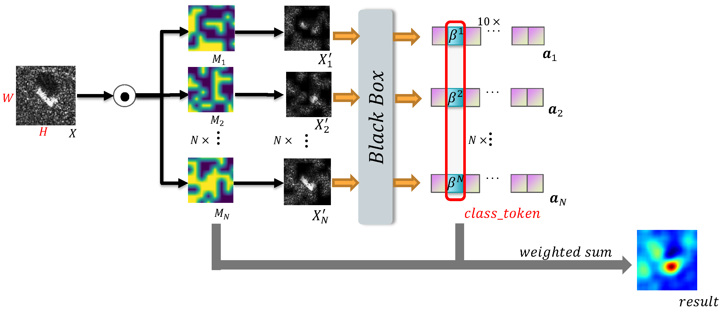
Figure 1.
The flowchart of RISE method.
Figure 1.
The flowchart of RISE method.
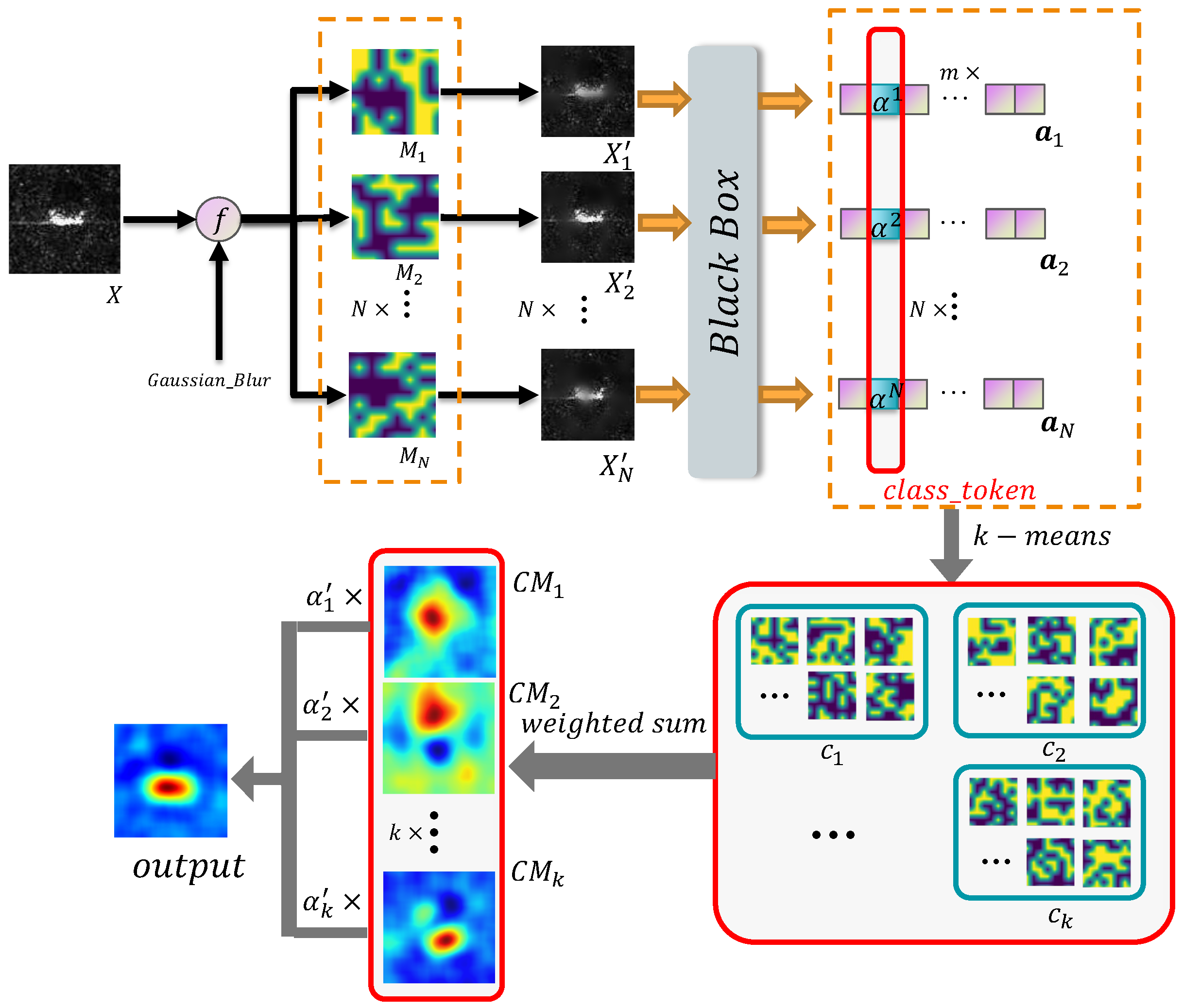
Figure 2.
The flowchart of C-RISE.
Figure 2.
The flowchart of C-RISE.
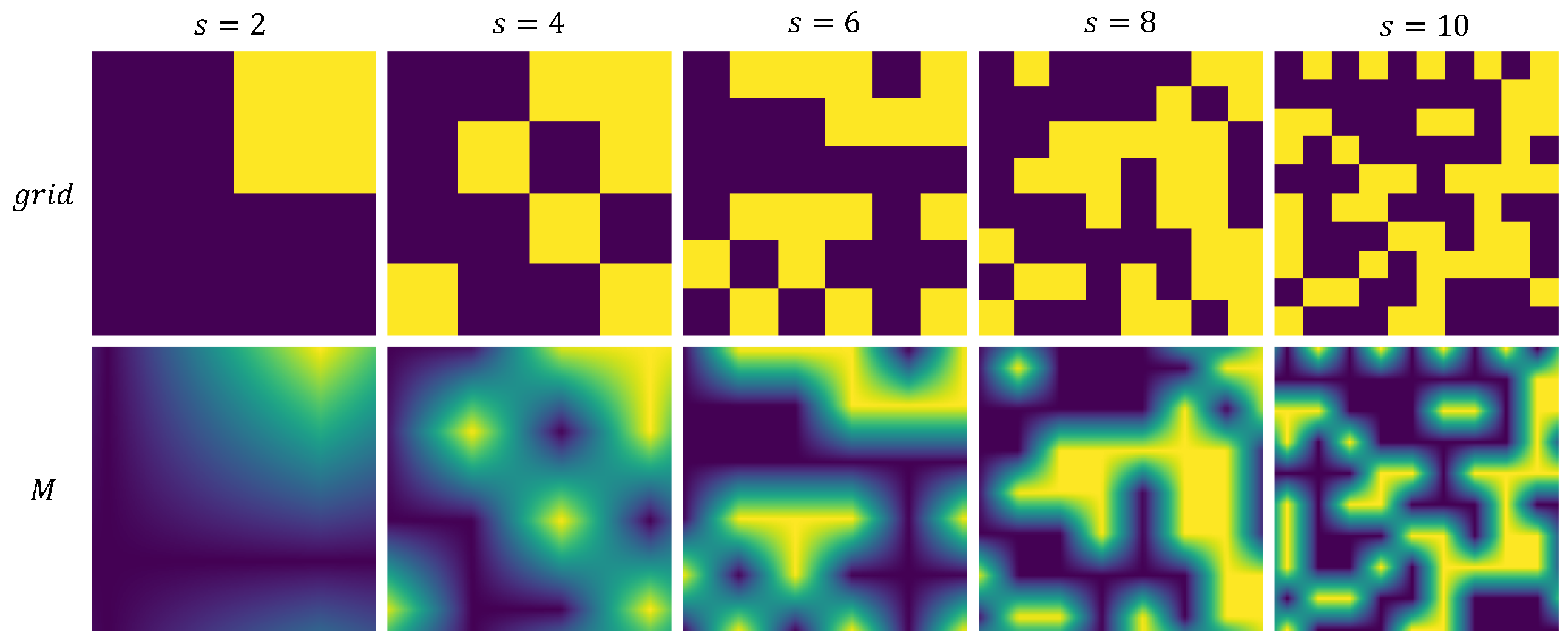
Figure 4.
Influence of different s on mask generation.
Figure 4.
Influence of different s on mask generation.
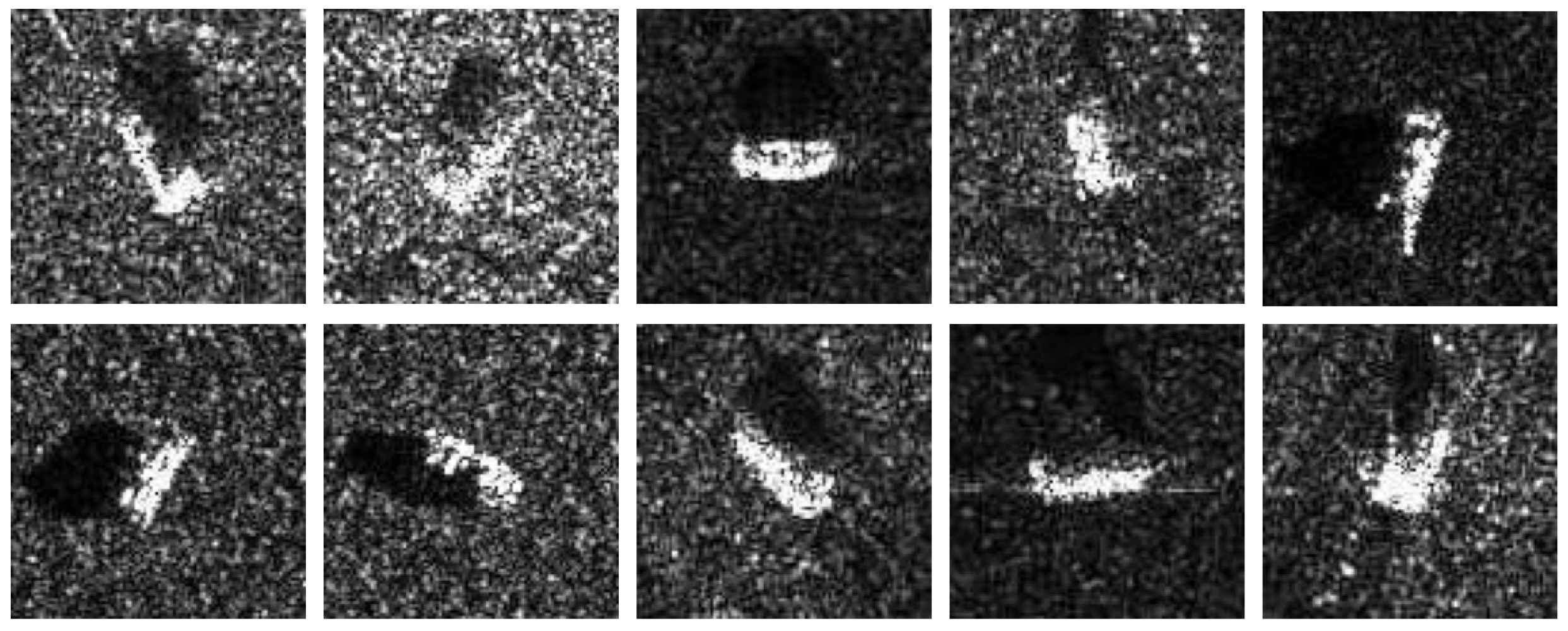
Figure 5.
10 typical SAR images for each category in MSTAR. The first row depicting random images from , , , , and , and the second row showing randomly selected images from , , , and .
Figure 5.
10 typical SAR images for each category in MSTAR. The first row depicting random images from , , , , and , and the second row showing randomly selected images from , , , and .
Figure 6.
The structure of Alexnet.
Figure 6.
The structure of Alexnet.
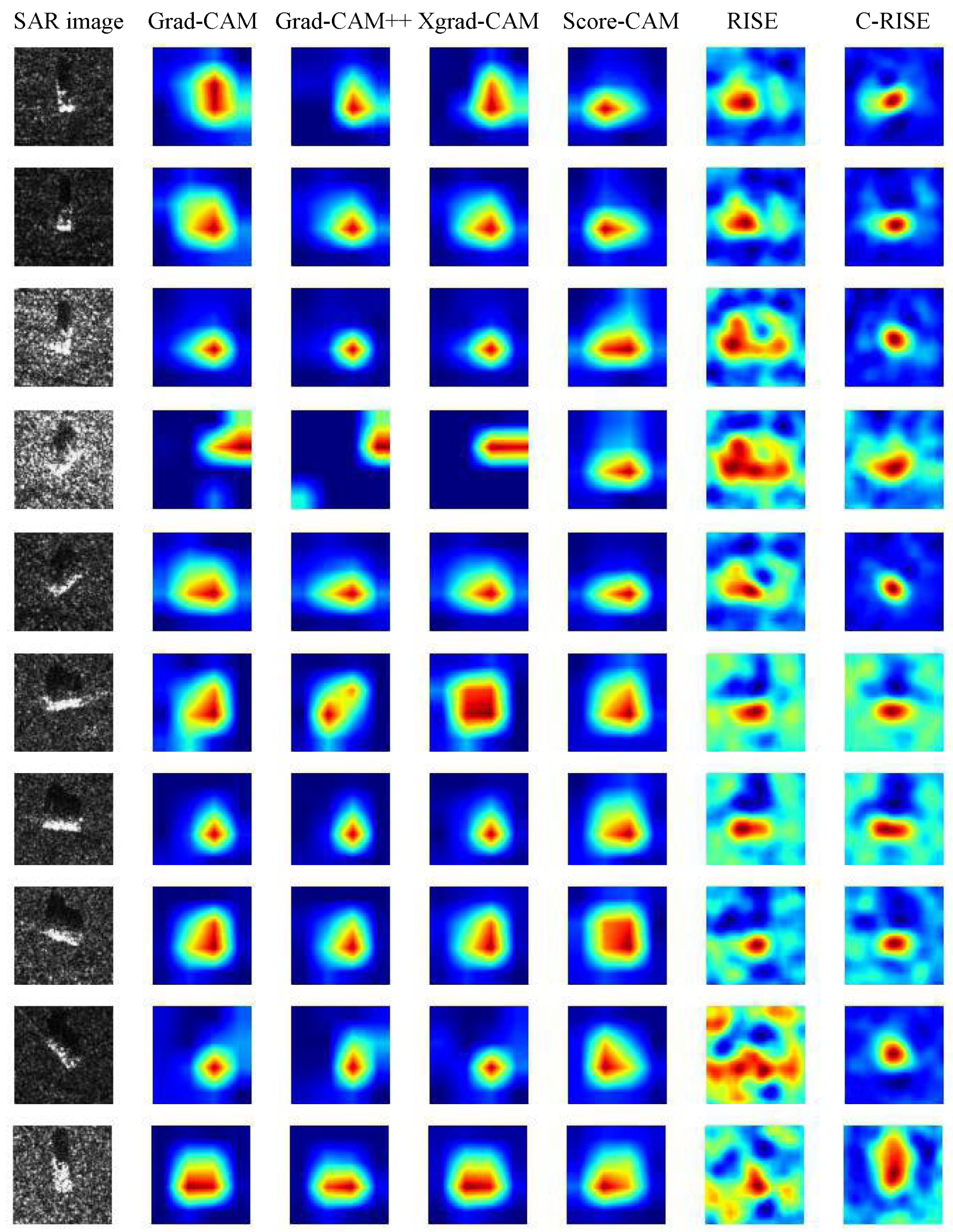
Figure 7.
Comparison of Grad-CAM, Grad-CAM++, XGrad-CAM, Score-CAM, RISE, C-RISE. The first column is the SAR images of ten classes. The rest of columns are corresponding heatmaps generated by each method respectively.
Figure 7.
Comparison of Grad-CAM, Grad-CAM++, XGrad-CAM, Score-CAM, RISE, C-RISE. The first column is the SAR images of ten classes. The rest of columns are corresponding heatmaps generated by each method respectively.
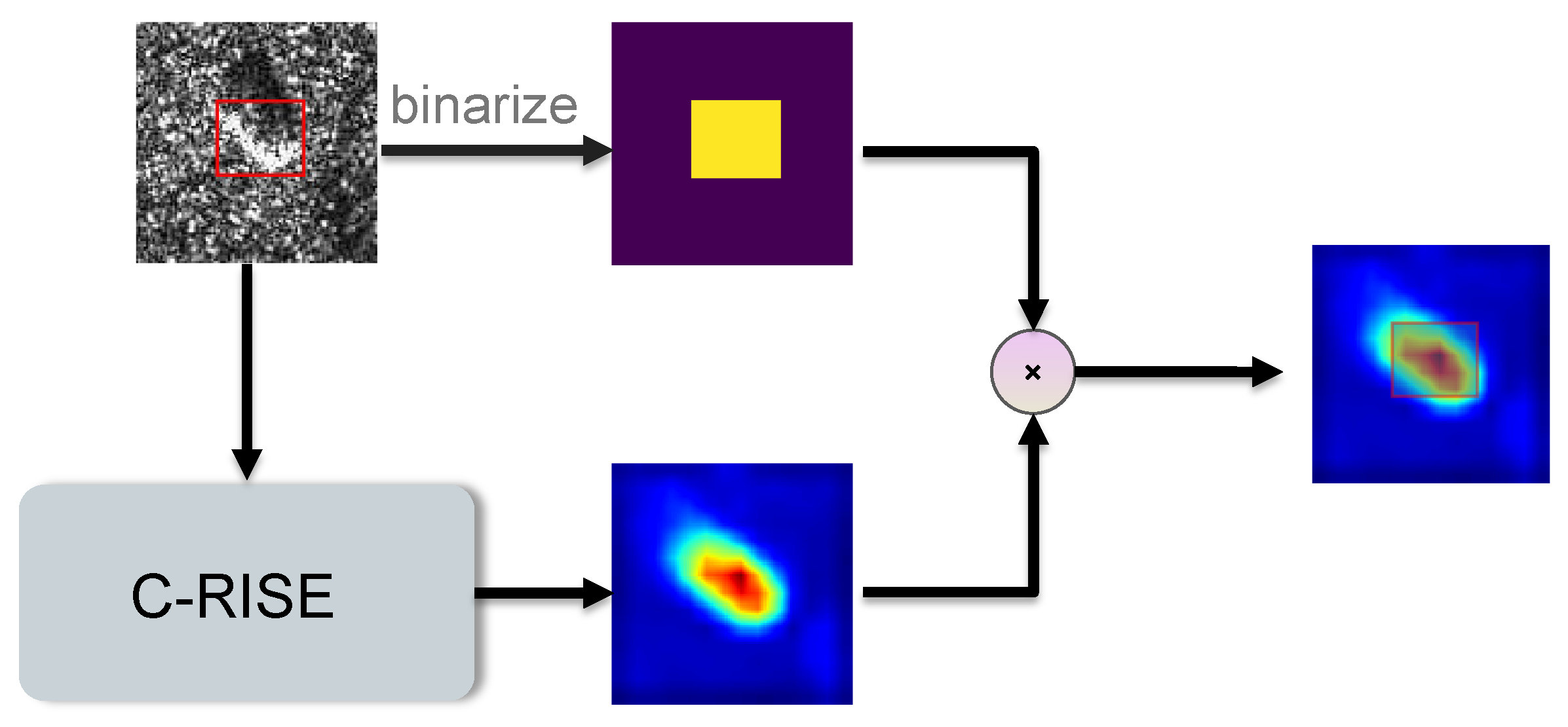
Figure 8.
The flowchat of calculating .
Figure 8.
The flowchat of calculating .
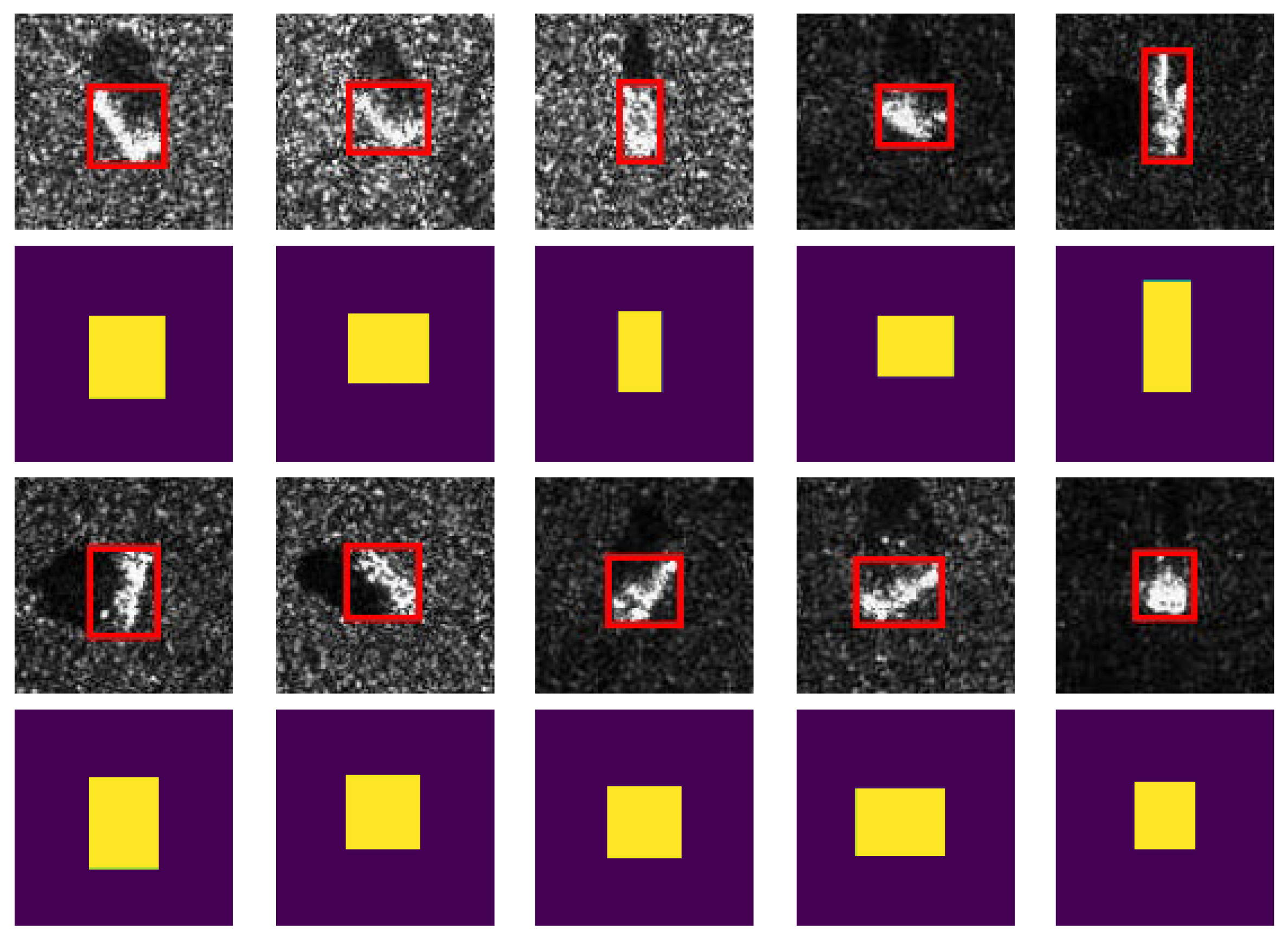
Figure 9.
The first and third rows represent randomly selected images with bounding boxes from 10 categories in the test set and the results of binarization of each images are shown as the second and fourth rows.
Figure 9.
The first and third rows represent randomly selected images with bounding boxes from 10 categories in the test set and the results of binarization of each images are shown as the second and fourth rows.
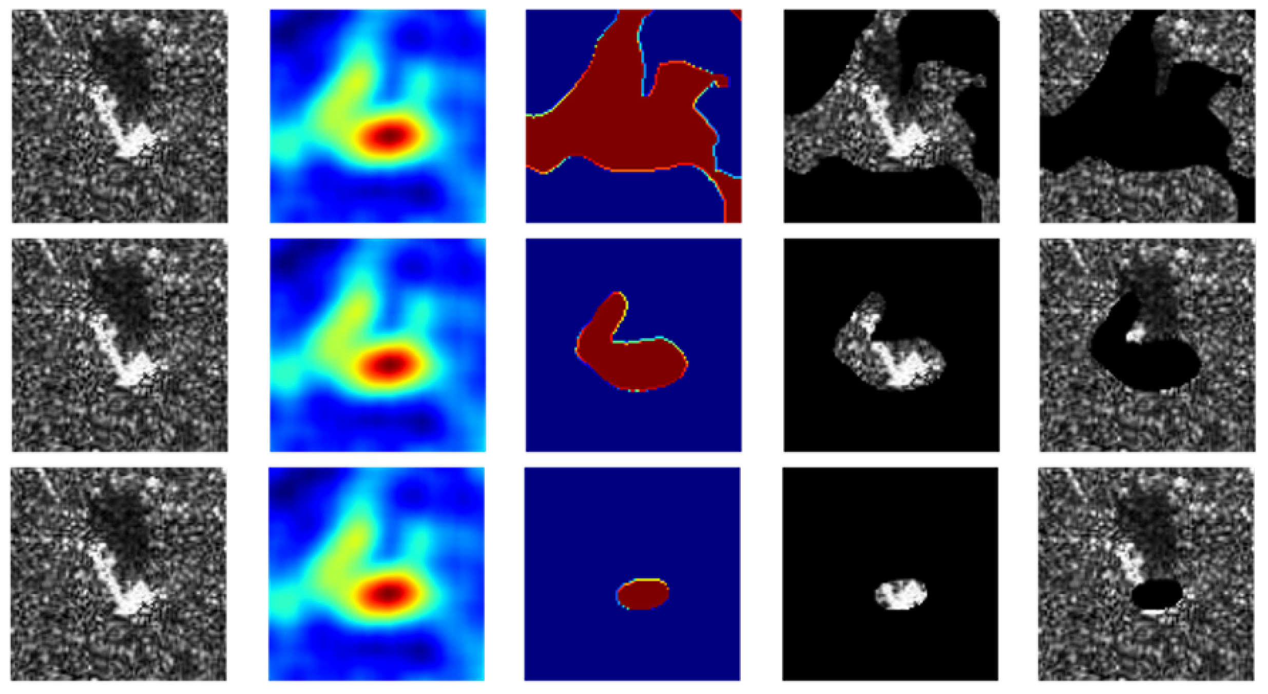
Figure 10.
The first column represents a randomly selected image from , the second column represents , the third column represents , and the fourth and fifth columns represent images after masked/reverse masked, respectively. The selected in the three lines were , and , respectively.
Figure 10.
The first column represents a randomly selected image from , the second column represents , the third column represents , and the fourth and fifth columns represent images after masked/reverse masked, respectively. The selected in the three lines were , and , respectively.
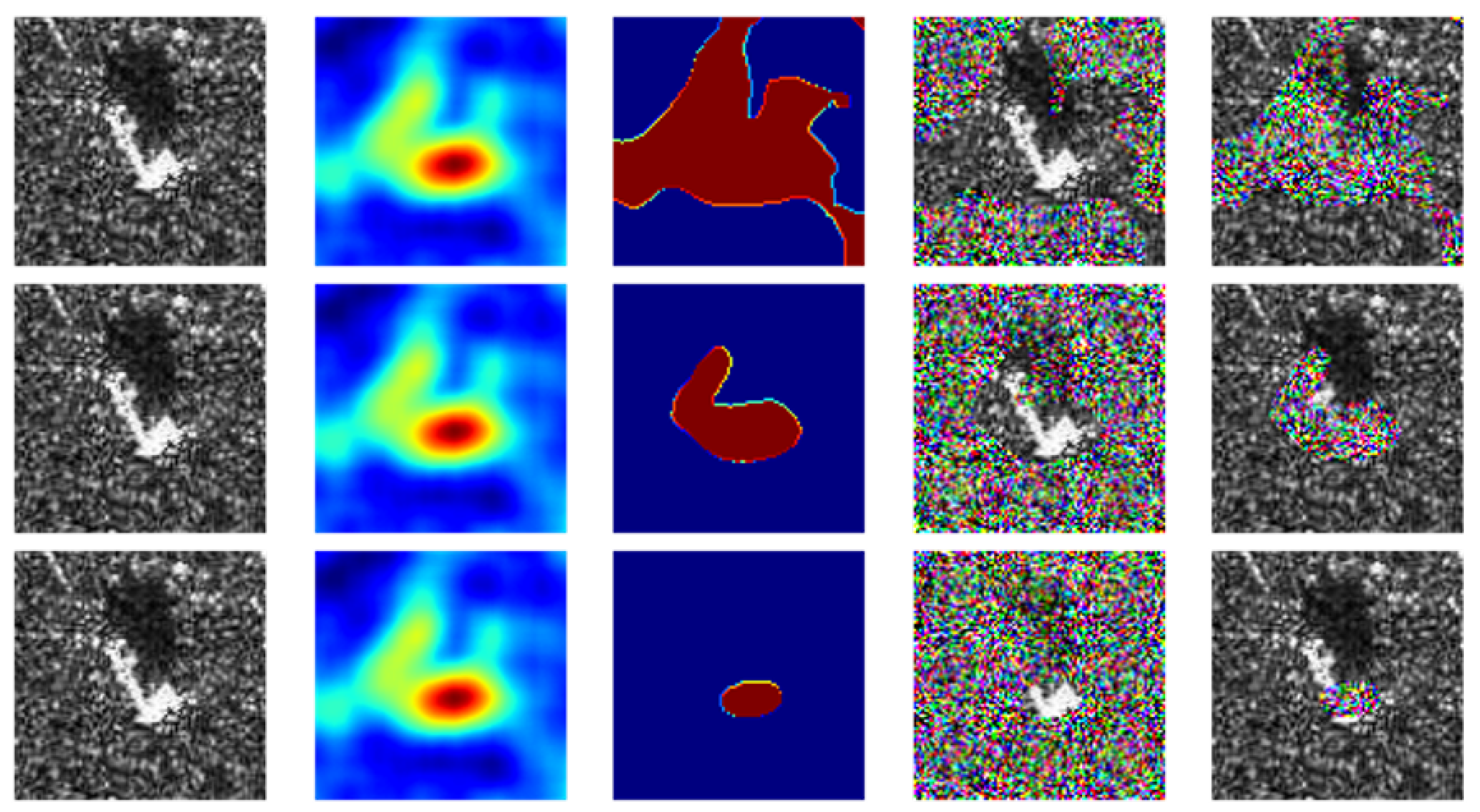
Figure 11.
The first column represents a randomly selected image from , the second column represents , the third column represents , and the fourth and fifth columns represent images after masked/reverse masked based on multiplicative noise, respectively. The selected in the three lines were , and , respectively.
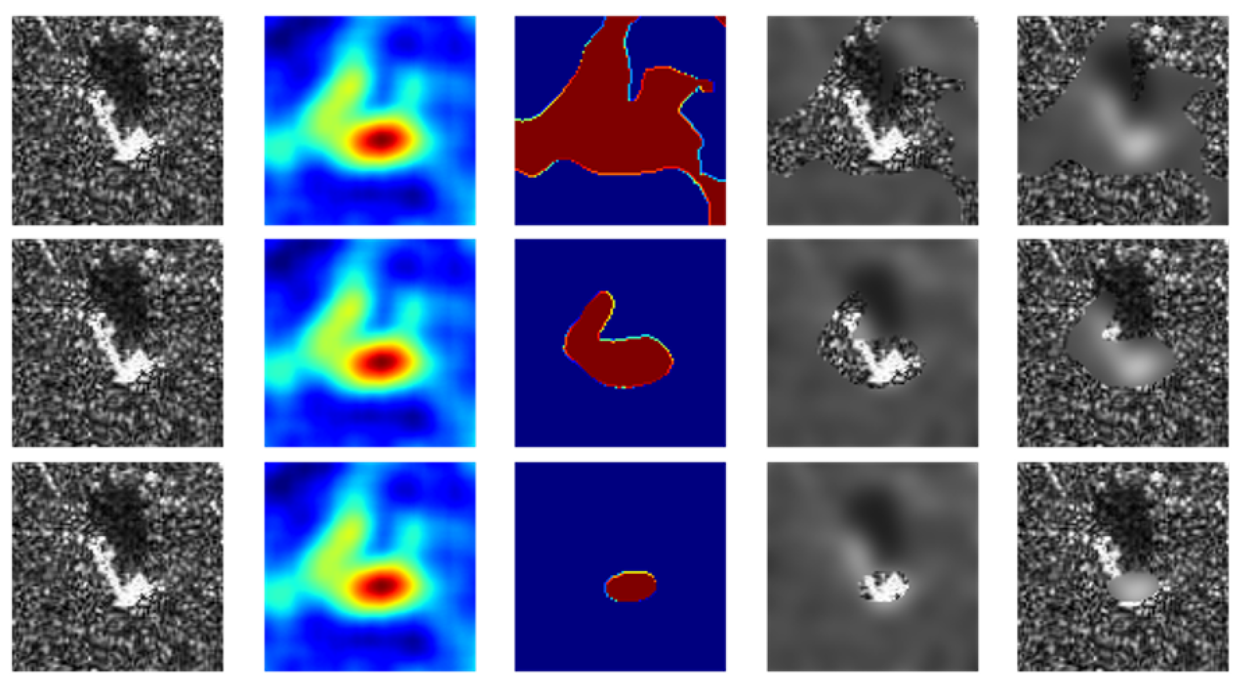
Figure 12.
The first column represents a randomly selected image from , the second column represents , the third column represents , and the fourth and fifth columns represent images after masked/reverse masked based on Gaussian blur, respectively. The selected in the three lines were , and , respectively.
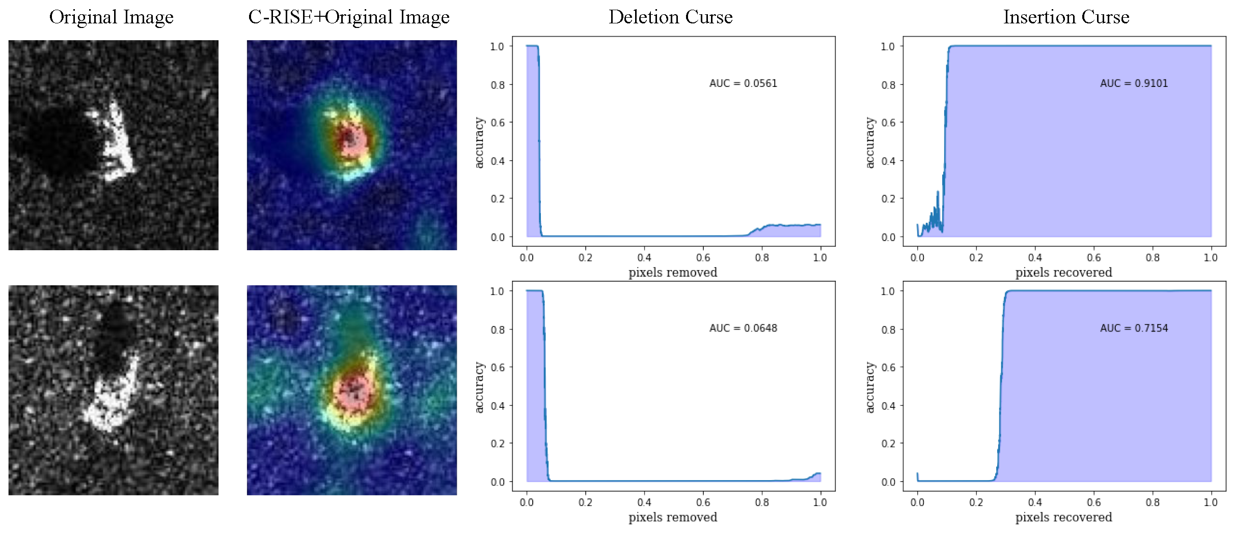
Figure 13.
The heatmap generated by C-RISE(second column) for two representative images (first column) with deletion (third column) and insertion (fourth column) curves.
Figure 13.
The heatmap generated by C-RISE(second column) for two representative images (first column) with deletion (third column) and insertion (fourth column) curves.
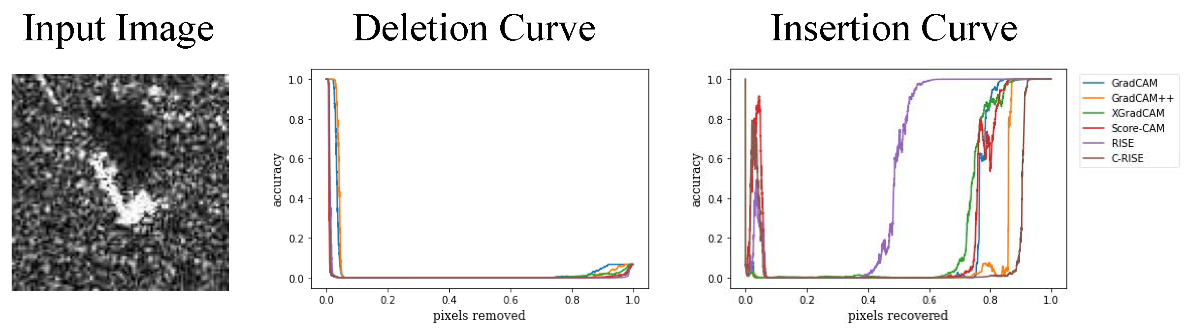
Figure 14.
Grad-CAM, Grad-CAM++, XGrad-CAM, Score-CAM, RISE and C-RISE generated saliency maps for a seleted image randomly (firstly column) in terms of deletion (second column) and insertion curves (third column).
Figure 14.
Grad-CAM, Grad-CAM++, XGrad-CAM, Score-CAM, RISE and C-RISE generated saliency maps for a seleted image randomly (firstly column) in terms of deletion (second column) and insertion curves (third column).
Figure 15.
Ablation studies of N with in terms of insertion (higher AUC is better ), deletion (lower AUC is better) curve and the over-all scores (higher AUC is better) on a subset of 100 randomly sampled images from the testset.
Figure 15.
Ablation studies of N with in terms of insertion (higher AUC is better ), deletion (lower AUC is better) curve and the over-all scores (higher AUC is better) on a subset of 100 randomly sampled images from the testset.
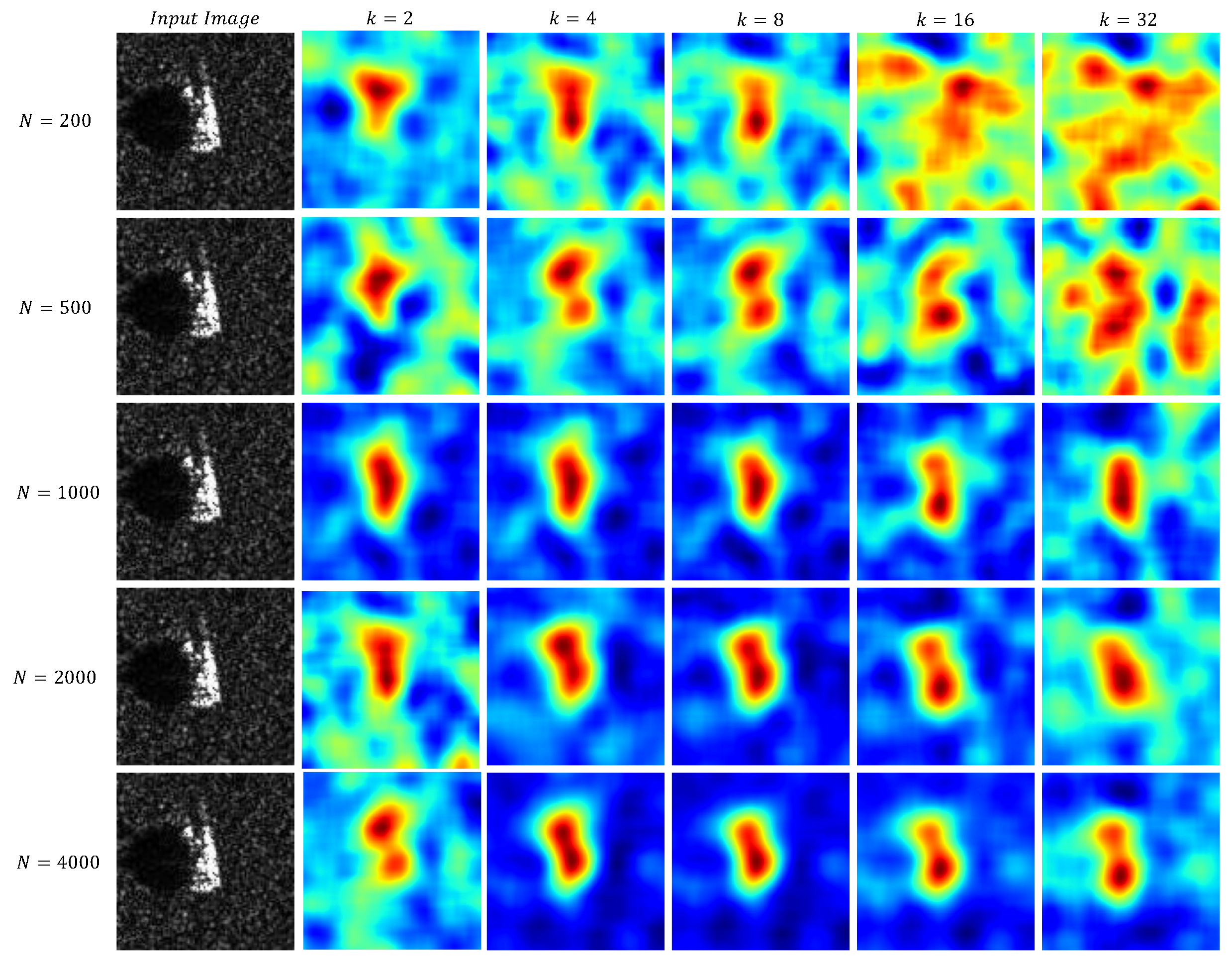
Figure 16.
The saliency maps which generated by a randomly selected image obtained using different combinations of N and k.
Figure 16.
The saliency maps which generated by a randomly selected image obtained using different combinations of N and k.
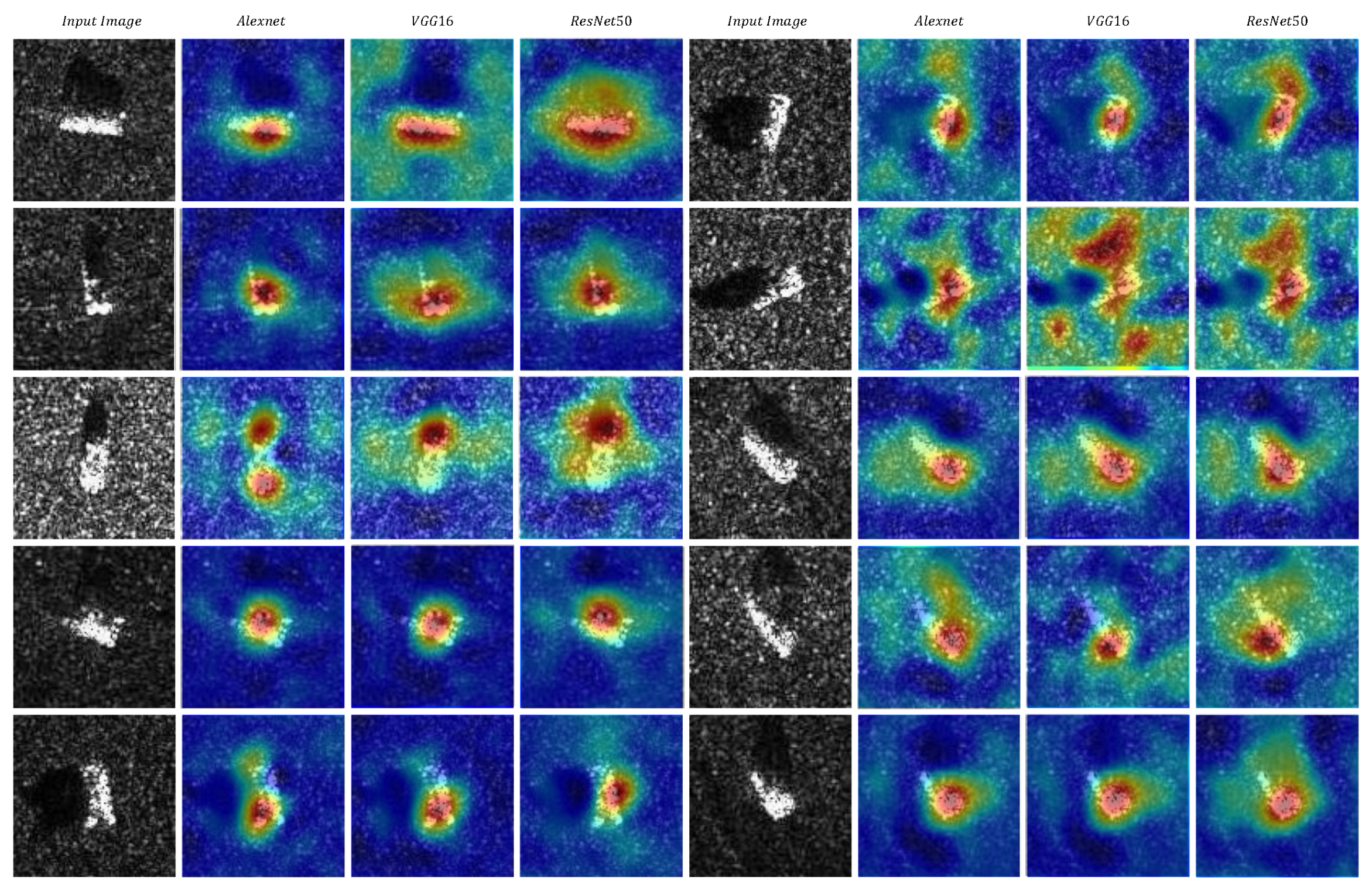
Figure 17.
The results obtained by applying the C-RISE algorithm to ten randomly selected images from ten different categories, using each of the aforementioned networks.
Figure 17.
The results obtained by applying the C-RISE algorithm to ten randomly selected images from ten different categories, using each of the aforementioned networks.
Table 1.
The of images in each category. The best records are marked in bold.
Table 1.
The of images in each category. The best records are marked in bold.
| | Grad-CAM | Grad-CAM++ | XGrad-CAM | Score-CAM | RISE | C-RISE |
|---|
| 2S1 | 0.5764 | 0.4252 | 0.5785 | 0.5524 | 0.3483 | 0.5876 |
| BRDM_2 | 0.5881 | 0.5138 | 0.5970 | 0.6230 | 0.3621 | 0.5930 |
| BTR_60 | 0.4355 | 0.3744 | 0.4553 | 0.3892 | 0.1024 | 0.4731 |
| D7 | 0.3782 | 0.6225 | 0.3920 | 0.5425 | 0.6406 | 0.4394 |
| SN_132 | 0.3820 | 0.5579 | 0.4168 | 0.4915 | 0.4797 | 0.4723 |
| SN_9563 | 0.4895 | 0.4024 | 0.4851 | 0.4421 | 0.2964 | 0.4817 |
| SN_C71 | 0.4121 | 0.2868 | 0.4409 | 0.3823 | 0.0856 | 0.4494 |
| T62 | 0.4975 | 0.3894 | 0.5158 | 0.4886 | 0.3374 | 0.5233 |
| ZIL131 | 0.5420 | 0.3984 | 0.5559 | 0.5265 | 0.4254 | 0.5498 |
| ZSU_23_4 | 0.4018 | 0.5315 | 0.4298 | 0.4616 | 0.5209 | 0.4474 |
| average | 0.4758 | 0.4555 | 0.4918 | 0.4976 | 0.3726 | 0.5060 |
Table 2.
of Different Methods in Conservation and Occlusion Test Based on Multiplicative Noise. The best records are marked in bold.
Table 2.
of Different Methods in Conservation and Occlusion Test Based on Multiplicative Noise. The best records are marked in bold.
| Threshold | Grad-CAM | Grad-CAM++ | XGrad-CAM | Score-CAM | RISE | C-RISE |
|---|
| 0.25 | 0.6975 | 0.6731 | 0.6949 | 0.7017 | 0.7364 | 0.6672 |
| 0.50 | 0.6750 | 0.7063 | 0.6760 | 0.6776 | 0.8257 | 0.6658 |
| 0.75 | 0.7620 | 0.7691 | 0.7644 | 0.7615 | 0.7646 | 0.6626 |
Table 3.
of Different Methods in Conservation and Occlusion Test Based on Multiplicative Noise. The best records are marked in bold.
Table 3.
of Different Methods in Conservation and Occlusion Test Based on Multiplicative Noise. The best records are marked in bold.
| Threshold | Grad-CAM | Grad-CAM++ | XGrad-CAM | Score-CAM | RISE | C-RISE |
|---|
| 0.25 | 0.7008 | 0.6434 | 0.6973 | 0.6427 | 0.4372 | 0.4934 |
| 0.50 | 0.3524 | 0.3287 | 0.4791 | 0.4804 | 0.1867 | 0.5361 |
| 0.75 | 0.1306 | 0.0475 | 0.1026 | 0.1359 | 0.1537 | 0.2637 |
Table 4.
of Different Methods in Conservation and Occlusion Test Based on Gaussian blur. The best records are marked in bold.
Table 4.
of Different Methods in Conservation and Occlusion Test Based on Gaussian blur. The best records are marked in bold.
| Threshold | Grad-CAM | Grad-CAM++ | XGrad-CAM | Score-CAM | RISE | C-RISE |
|---|
| 0.25 | 0.0665 | 0.1038 | 0.0768 | 0.0205 | 0.0137 | 0.0064 |
| 0.50 | 0.0285 | 0.2391 | 0.1764 | 0.0944 | 0.0924 | 0.1692 |
| 0.75 | 0.3147 | 0.3721 | 0.3249 | 0.2893 | 0.2466 | 0.1631 |
Table 5.
of Different Methods in Conservation and Occlusion Test Based on Multiplicative Noise. The best records are marked in bold.
Table 5.
of Different Methods in Conservation and Occlusion Test Based on Multiplicative Noise. The best records are marked in bold.
| Threshold | Grad-CAM | Grad-CAM++ | XGrad-CAM | Score-CAM | RISE | C-RISE |
|---|
| 0.25 | 0.2805 | 0.2250 | 0.2682 | 0.3283 | 0.3898 | 0.3985 |
| 0.50 | 0.1634 | 0.0968 | 0.1519 | 0.2217 | 0.2513 | 0.2870 |
| 0.75 | 0.0350 | 0.0119 | 0.0305 | 0.0556 | 0.0906 | 0.1663 |
Table 6.
Comparative evaluation in terms of deletion (lower is better) and insertion (higher AUC is better) . The score (higher is better) shows that C-RISE outperform other related methods significantly. The best records are marked in bold.
Table 6.
Comparative evaluation in terms of deletion (lower is better) and insertion (higher AUC is better) . The score (higher is better) shows that C-RISE outperform other related methods significantly. The best records are marked in bold.
| Grad-CAM | Grad-CAM++ | XGrad-CAM | Score-CAM | RISE | C-RISE |
|---|
| Insertion | 0.2768 | 0.3011 | 0.4145 | 0.5512 | 0.4659 | 0.6875 |
| Deletion | 0.1317 | 0.1676 | 0.1255 | 0.0246 | 0.0420 | 0.1317 |
| Over_All | 0.1451 | 0.1335 | 0.2890 | 0.5266 | 0.4239 | 0.5558 |
Table 7.
Ablation studies of k with in terms of insertion (higher AUC is better ), deletion (lower AUC is better) curve and the over-all scores (higher AUC is better) on a subset of 100 andomly sampled images from the testset.
Table 7.
Ablation studies of k with in terms of insertion (higher AUC is better ), deletion (lower AUC is better) curve and the over-all scores (higher AUC is better) on a subset of 100 andomly sampled images from the testset.
| | | | | |
|---|
| Insertion | 0.5687 | 0.7140 | 0.5076 | 0.5329 | 0.4619 |
| Deletion | 0.0942 | 0.0910 | 0.1697 | 0.1753 | 0.1783 |
| Over_All | 0.4745 | 0.6230 | 0.3379 | 0.3576 | 0.2836 |


 ,
, 


