Investigation into the Affect of Chemometrics and Spectral Data Preprocessing Approaches upon Laser-Induced Breakdown Spectroscopy Quantification Accuracy Based on MarSCoDe Laboratory Model and MarSDEEP Equipment

Abstract

As part of China’s Tianwen-1 Mars mission, the Mars Surface Composition Detector (MarSCoDe) instrument on the Zhurong rover adopts laser-induced breakdown spectroscopy (LIBS) to perform chemical component detection of the materials on the Martian surface. However, it has always been a challenging issue to achieve high accuracy in LIBS quantification. This study investigated the effect of chemometrics and spectral data preprocessing approaches on LIBS quantification accuracy based on different chemometrics algorithms and diverse preprocessing methods. A total of 2340 LIBS spectra were collected from 39 kinds of geochemical samples by a laboratory duplicate model of the MarSCoDe instrument. The samples and the MarSCoDe laboratory model were placed in a simulated Martian atmosphere environment based on equipment called the Mars-Simulated Detection Environment Experiment Platform (MarSDEEP). To quantify the concentration of MgO in the samples, we employed two common LIBS chemometrics; i.e., partial least squares (PLS) and a back-propagation neural network (BPNN). Meanwhile, in addition to necessary routine preprocessing such as dark subtraction, we used five specific preprocessing approaches, namely intensity normalization, baseline removal, Mg-peak wavelength correction, Mg-peak feature engineering, and concentration range reduction. The results indicated that the performance of the BPNN was better than that of the PLS and that the preprocessing of Mg-peak wavelength correction had the most prominent effect to improve the quantification accuracy. The results of this study are expected to provide inspiration for the processing and analysis of the in situ LIBS data acquired by MarSCoDe on Mars.

1. Introduction

During China’s first Mars exploration mission, namely the Tianwen-1 mission, the Tianwen-1 lander successfully landed on the Utopia Plain of Mars (25.06°N, 109.92°E) in May 2021, and the Zhurong rover begun scientific investigations around the landing site thereafter [1]. There are six major scientific loads on the Zhurong rover aiming to analyze the topography and geological structure, the soil structure (profile) and water ice, the surface elements, minerals, rock types, the atmospheric physical characteristics, and the surface environment of Mars. As one of the primary payloads, the Mars Surface Composition Detector (MarSCoDe) can detect the chemical composition of the Martian substances using laser-induced breakdown spectroscopy (LIBS), short-wave infrared spectroscopy (SWIR), and micro-imaging [2]. The LIBS technique is used to identify the types of rocks and soils on Martian surface and quantify the element concentration of those materials [3].

LIBS is an atomic emission spectroscopy technology [4]. The surface of a sample is ablated, melted, and vaporized by focusing a high-energy laser pulse on the target, then a plasma formed on the surface due to a large number of material atoms is ionized. The advantage of LIBS is that it can analyze various substances in solid, liquid, gas, and colloidal states [5]. It is able to perform rapid detection of samples without special sample pretreatment, so LIBS has been widely used.

LIBS has become an excellent tool for planetary detection due to the ability of remote detection. The special surface environment of Mars is very different from that of Earth, and LIBS can remove dust from the rock surface and has a wide detection range of elements, making it a technology with great advantages in deep space exploration [6]. At present, many LIBS devices have been equipped on the payloads of Mars exploration missions such as the Curiosity rover and the Perseverance rover launched by the National Aeronautics and Space Administration (NASA) [7,8] and the Zhurong rover of China.

LIBS devices have made some achievements in the field of deep space exploration at present. LIBS cooperates with an alpha particle X-ray spectrometer (APXS) on Curiosity to measure elemental abundances. They provide supplementary data by revealing the composition of rocks and components that can be directly related to texture characteristics [9]. Using the remote chemical analysis capability of LIBS, which is especially sensitive to various elements (including hydrogen), can help us reveal the formation time of clay minerals [10]. The LIBS device on Perseverance assists other devices to analyze the compositionally and density stratified igneous rock terrain of the Jezero crater, helping to deduce the formation process of the crater [11]. Combined with the LIBS and SWIR spectral analysis of MarSCoDe, the composition and mineralogy of the Vastitas Borealis Formation at the landing site of Tianwen-1 were studied, providing basic facts and further constraints regarding the genesis of the Vastitas Borealis Formation. The research results largely supported the hypotheses of a frozen ocean and sublimation [12].

The spectrum signal intensity obtained by LIBS is related to the element content, so the spectrum intensity can be used for the quantitative analysis of elements. Different kinds of matrix effects [13], the self-absorption effect [14], equipment performance, fluctuations in experimental conditions and other factors [15], and the broadening mechanism of spectrum lines will make LIBS spectra unstable. The wavelength position of the element characteristic spectrum lines will shift and the spectrum line intensity will also change, which makes the quantitative analysis of LIBS spectra difficult.

In traditional LIBS quantitative analysis, researchers usually adopt classical statistical methods such as partial least squares (PLS) [16] and principal component regression (PCR) [17]. The results yielded by these methods have good stability and strong interpretability but are generally not accurate enough due to their inherent nature of linearity. With the development of machine learning in the past decades, machine learning/deep learning-based methods have been widely employed in LIBS quantification studies and demonstrated their superiority over traditional methods in terms of accuracy [18,19].

The SuperCam team used ordinary least squares (OLS), random forest (RF), PLS, ridge regression (Ridge), elastic net (ENet), and other methods in the quantitative analysis of elements [20]. The final analysis method was selected according to the quantitative analysis accuracy of the element under different methods. The SuperCam team improved the accuracy of quantification by trying different methods. All spectra were pretreated under the same methods. Patrick et al. used the data obtained by ChemCam for the quantitative analysis of the Mn element. They found that a multivariable model, which greatly improved the accuracy compared with the single-variable model, could distinguish small changes in MnO [21]. Except in the field of deep space exploration, machine learning has also been applied to the quantitative analysis of LIBS. Zhang et al. used random forest regression (RFR) to quantify multiple elements in steel and obtained better prediction results than PLS and support vector machines (SVMs), which confirmed a good potential of RFR combined with LIBS [22].

Generally speaking, a LIBS spectral profile depends highly on atmospheric environment parameters such as gas composition, pressure, temperature, and so on. The atmospheric parameters of Mars are quite different from those of the Earth, so LIBS data obtained in an ordinary laboratory environment might not be able to assist well in analyzing the LIBS spectra collected on Mars due to their considerable spectral profile differences. The ChemCam team has developed a laboratory that can simulate the atmospheric environment of Mars. They can use the ChemCam laboratory model to collect LIBS spectra in the laboratory, which makes better use of the data collected by ChemCam on Mars [23]. A large planetary simulation chamber called Andromeda has also been built at the Arkansas–Oklahoma Center for Space and Planetary Science [24].

The existing planetary simulation facilities mentioned above can only place the samples in a vacuum environment while the detection instruments are still in the normal air environment, which cannot completely simulate the working environment of the instruments on Mars. The signal must be received by the detector through a specific transmission window, which can easily cause distortions of the signal. In order to make better use of the data collected on Mars, we employed a specially built LIBS experimental facility, namely the Mars-Simulated Detection Environment Experiment Platform (MarSDEEP), which is able to simulate the Martian atmospheric environment. In addition to MarSDEEP, we also have a MarSCoDe laboratory model that is a duplicate of the MarSCoDe flight model on the Zhurong rover, and the technical parameters of the two instruments are almost identical. In addition to the simulation of atmospheric pressure, gas composition, and temperature, we can use the advantages of the large size of the experimental platform to place samples and instruments in the vacuum chamber [25], hence we can simulate the filed detection of MarSCoDe on Mars to the maximum extent.

Based on the LIBS spectra collected in the Mars-simulated environment, we carried out a quantitative analysis in this study using two chemometrics; i.e., PLS and a back-propagation neural network (BPNN), which are representative of classical methods and machine learning methods, respectively. In addition to comparing the analytical chemometrics, we also used five specific spectral preprocessing approaches and investigated their effects on the quantification accuracy. In Section 2, the details of the LIBS experiments and spectral data processing methods are presented. The results of the quantitative analysis are then stated and discussed in Section 3. Finally, the conclusions are provided in Section 4.

2. Experimental Methods

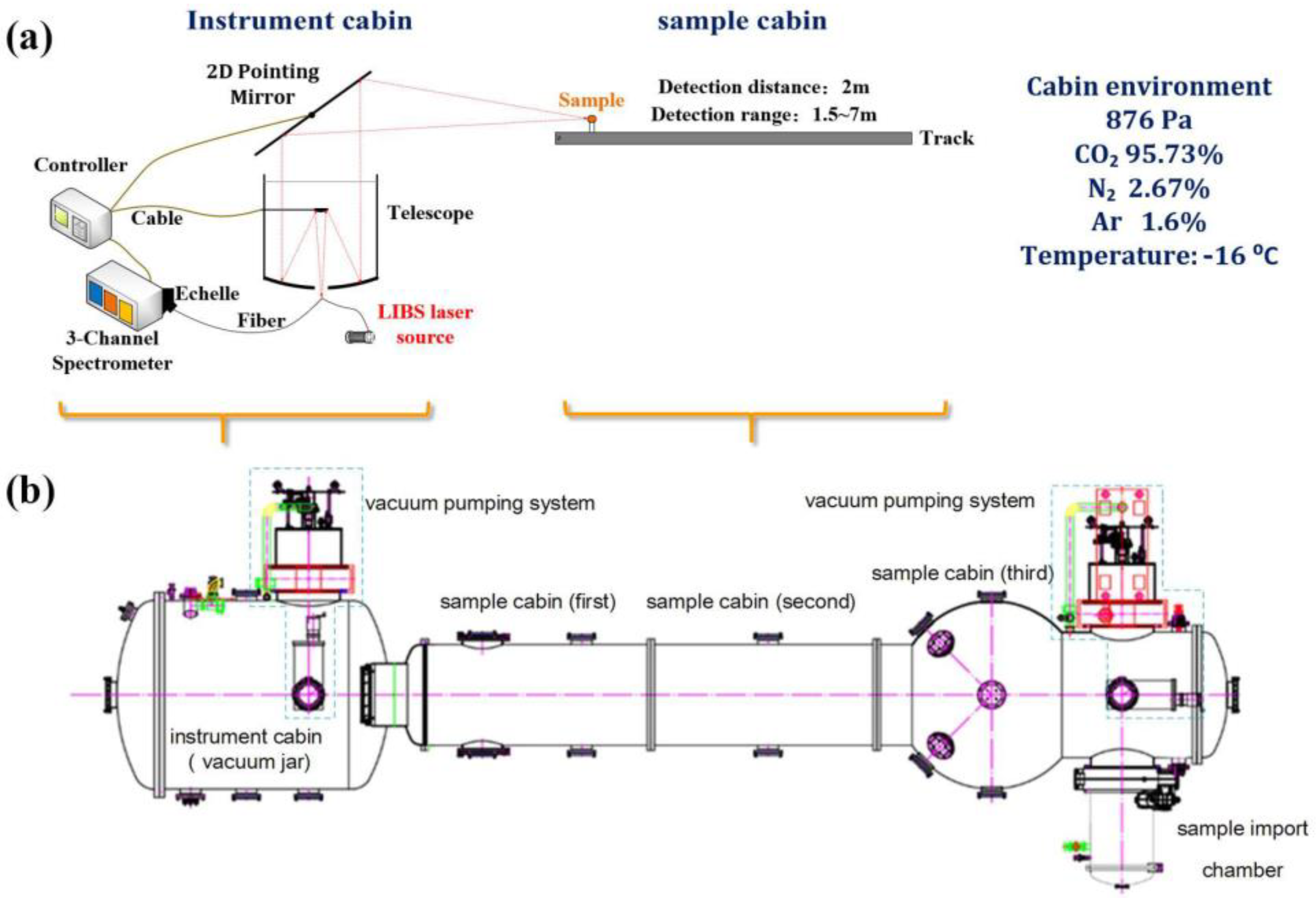
2.1. Experimental Setup

In this study, all the LIBS spectra were acquired by the MarSCoDe laboratory model, and both the instrument and the target samples were placed in the Mars-like atmospheric environment simulated by MarSDEEP. The schematic diagram of MarSDEEP and the operating principle of MarSCoDe are shown in Figure 1. The experimental platform had a three-segment structure consisting of an approximate spherical part and two cylindrical parts. The experimental platform comprised an instrument cabin (or called a vacuum jar), a sample cabin, a sample import chamber, and a 3D vacuum stage. In the experiment, the MarSCoDe laboratory model was placed in the instrument cabin, and the samples were placed on the sample stage in the sample cabin. Inside the sample cabin, there was a track along which the sample stage could move in the cabin, hence enabling the LIBS detection distance to vary from 1.6 to 7 m.

With a vacuum pumping system, a temperature control system, an atmospheric simulation system, a measurement and control system, and other auxiliary equipment, it could simulate the pressure, temperature, and gas composition of Mars. All the cabins were connected, so the instruments and samples were in the same environment.

MarSDEEP had two identical pump sets at either end of the cabin. One set of vacuum pump included an oilless dry pump (HANBELL PS-160, Shanghai, China), a magnetic suspension molecular pump (SHIMADZU TMP 1003LM, Kyoto, Japan), and a cryogenic pump (ULVAC CRUYO-U20PN, Kanagawa Prefecture, Japan); the limit vacuum degree achievable in the cabin could reach 10⁻⁵ Pa level.

The temperature control system was composed of a heating system and a liquid nitrogen cooling system that were distributed between the heat sink and the inner wall of the cabin. This design ensured that the samples and instrument were heated or cooled at the same time so that their temperatures were consistent. Several temperature-monitoring probes were installed at different positions in the instrument cabin and sample cabin that could monitor and intelligently adjust the temperature inside the cabin. The temperature could vary from −190 °C to +180 °C under good control.

The atmospheric simulation system included a gas filling and mixing unit and a quadrupole mass spectrometer so it could fill different gases in proportion to simulate the Mars atmospheric environment. The quadrupole mass spectrometer could monitor the composition and proportion of gases in the cabin in real time.

The detection distance selected for this experiment was 2 m; the pressure of the simulated Mars environment was 876 Pa; the temperature was −16 °C; and the filling gas was composed of 95.73% CO₂, 2.67% N₂, and 1.6% Ar (volume percentage). After many attempts, the experimental platform could well simulate the experimental environment of LIBS instrument in situ exploration on Mars.

In order to achieve high-degree simulation of the in situ exploration on Mars, the LIBS instrument used in the laboratory was almost identical to the technical specifications of MarSCoDe. All spectra were collected in a simulated Mars environment. In Figure 1, it can be seen that MarSCoDe pointed the laser at the target and received the emitted light from the sample through a 2D pointing mirror. For high-wavelength resolution for the entire spectral range, MarSCoDe adopted a three-channel spectrometer system. The main parameters of the MarSCoDe instrument are listed in

Table 1. Main parameters of MarSCoDe.

Parameter	Value
Stand-off distance	1.6–7.0 m
Laser type	Nd:YAG
Pulse width	4 ns
Pulse energy	9 mJ
Pulse repetition rate	1–3 Hz
Laser wavelength	1064 nm
Entire spectral range	240–850 nm
SSI of each channel	0.1 nm at 240–340 nm
	0.2 nm at 340–540 nm
	0.3 nm at 540–850 nm

. The LIBS excitation laser had a wavelength of 1064 nm, a pulse width of 4 ns, and a pulse energy of 9 mJ. The band ranges of the three spectral channels were 240–340 nm, 340–540 nm, and 540–850 nm, respectively. Each channel had 1800 pixels, and hence an entire LIBS spectrum consisted of 5400 pixel data points. The wavelength difference corresponding to two adjacent pixels in one channel was defined as the spectral sampling interval (SSI), which was considered constant within each channel.

2.2. Sample Preparation and Spectra Collection

A total of 39 geochemical samples were employed in this LIBS experiment, including 35 national reference material samples and 4 self-made samples. To investigate the effect of the chemometrics, we selected MgO as the component for quantitative analysis since it is a metal oxide commonly existed in Martian materials. Indeed, besides MgO, some other oxides such as FeO_T, SiO₂, etc., are also common in Martian materials. However, it was hoped that the selected component could be contained in as many target samples as possible in our experiment so that the total dataset for the chemometrics could be large. For the 39 samples herein, the MgO component existed in every sample, and the concentration was not too low (>0.05%). Other oxides such as FeO_T and SiO₂ only existed in a portion of the samples or had too low of a concentration. If those components were chosen, the number of samples in the dataset would be reduced and hence the performance of the chemometrics might degrade. Moreover, since Mg is a highly active metal, the characteristic peaks of Mg usually had a high signal-to-noise ratio in our LIBS spectra, and this fact was important for the subsequent specific spectral preprocessing. Considering the above two main factors, we finally selected MgO to examine the quantification accuracy of our LIBS chemometrics in this work.

The initial state of the samples was a uniform powder. For each sample, 3 g of powder was weighed and pressed at 30 MPa for 90 s, yielding a tablet with a diameter of 40 mm and a thickness of 6 mm. As a matter of fact, the calibration targets on the MarSCoDe instrument were sintered powder samples instead of pressed powder ones. This also was true for the SuperCam calibration targets. The MarSCoDe team and the SuperCam team adopt sintered samples as calibration targets because sintered samples have higher solidity than pressed ones and they can better withstand the mechanical vibrations and impacts during launch and landing processes. For laboratory experiments, however, the requirement for the sample solidity is not that high. So, pressing was adopted rather than sintering in this study because pressing is simpler and free of high temperature procedures. In fact, in the laboratory experiments of the SuperCam team, most of the targets were also pressed powder samples, and only those targets with identical composition to the SuperCam calibration targets were sintered samples.

Some of the pressed samples and the sample stage used in the experiment are shown in Figure 2.

The MgO component concentration distribution of all the 39 samples is listed in

Table 2. The information on the 39 target samples used in our LIBS experiment. Sample Nos. 1 to 4 were self-made samples offered by Shanghai Jiao Tong University. Sample Nos. 5 to 39 were national reference materials, and the reference IDs are displayed in the table. The MgO content value for each sample is expressed in weight percentage (in unit of %).

No.	Material	Reference ID	MgO Content
1	Andesite	NA	0.43
2	Rhyodacite	NA	0.057
3	Trachyte	NA	2.96
4	Olivine basalt	NA	10.05
5	Andesite	GBW07104(GSR-2)	1.72
6	Basalt variant type-I	GBW07105(GSR-3)	7.77
7	Kaolin	GBW03121a	0.069
8	Soft clay	GBW03115	0.3
9	Copper rich ore	GBW07164(GSO-3)	2.33
10	Lead ore type-I	GBW07235	1.62
11	Carbonate rock	GBW07127	6.76
12	Dolomite	GBW07217a	20.37
13	Yellow-red soil	GBW07405(GSS-5)	0.61
14	Latosol	GBW07407(GSS-7)	0.26
15	Stream sediment type-I	GBW07309(GSD-9)	2.39
16	Stream sediment type-VII	GBW07311(GSD-11)	0.62
17	Granitic gneiss	GBW07121(GSR-14)	1.63
18	Clay	GBW03101a	0.46
19	Shale type-I	GBW03104	0.67
20	Argillaceous limestone	GBW07108(GSR-6)	5.19
21	Polymetallic ore	GBW07163(GSO-2)	1.39
22	Floodplain sediment	GBW07390(GSS-34)	2.66
23	Shale type-II	GBW07107(GSR-5)	2.01
24	Nickel ore	GBW07146	14.56
25	Polymetallic lean ore	GBW07162(GSO-1)	1.55
26	Lead ore type-II	GBW07236	2.06
27	Molybdenum ore	GBW07239	1.83
28	Stream sediment type-III	GBW07305a(GSD5a)	1.29
29	Stream sediment type-IV	GBW07307a(GSD7a)	2.5
30	Stream sediment type-V	GBW07308a(GSD8a)	0.47
31	Saline-alkali soil type-I	GBW07447(GSS-18)	2.58
32	Sierozem	GBW07450(GSS-21)	2.04
33	Quartz sandstone	GBW07106(GSR-4)	0.082
34	Saline-alkali soil type-II	GBW07449(GSS-20)	2.98
35	Stream sediment type-II	GBW07377(GSD-26)	1.73
36	Lead–zinc rich ore	GBW07165(GSO-4)	0.59
37	Granite	GBW07103(GSR-1)	0.42
38	Siliceous sandstone	GBW03112	0.066
39	Stream sediment type-VI	GBW07310(GSD10)	0.12

. Every concentration value is expressed in terms of weight percentage (for simplicity, we just use “%” instead of “wt.%” in this text).

Each sample was irradiated by 60 laser pulses in the simulated Mars environment, and hence 60 LIBS spectra were collected. Immediately after the LIBS spectra acquirement for each sample, three non-laser spectra were collected. These non-laser spectra were utilized to calculate the dark background for the subsequent spectral preprocessing. During the experiment, the sample stage rotated at a small angle at a time to realize the alternation of samples, as demonstrated in Figure 2b. There were 16 sample positions on the stage, but no more than 15 target samples were placed at a time because there was always a position reserved for a specially made Ti-alloy sample. The spectra of this special Ti sample would play a key role in wavelength drift correction (see Section 2.3.2). In total, 2340 LIBS spectra were acquired from the 39 target samples.

Before being analyzed using chemometrics, the LIBS spectra underwent a series of spectral preprocessing steps, as elucidated in the next section.

2.3. Data Preprocessing

In this study, spectral preprocessing was divided into two types; i.e., preliminary preprocessing and additional specific preprocessing. The preliminary preprocessing steps included dark subtraction, wavelength calibration and drift correction, and ineffective pixel screening and channel splicing, as described in Section 2.3.1, Section 2.3.2 and Section 2.3.3. The spectra after the preliminary preprocessing are called original spectra in this paper.

Based on the original spectra, five different specific preprocessing approaches were used to investigate the effect of preprocessing. The five specific preprocessing were intensity normalization, baseline removal, Mg-peak wavelength correction, Mg-peak feature engineering, and concentration range reduction, as described in Section 2.3.4, Section 2.3.5, Section 2.3.6, Section 2.3.7 and Section 2.3.8. Note that the five additional preprocessing schemes were generally independent of each other. In other words, they were “parallel” rather than “cascaded”, and we only implemented one of them at a time on the basis of the original spectra.

2.3.1. Dark Subtraction

In the process of collecting spectral information, the electronic components of CCD have a dark current and stray light may be introduced into the optical system, yielding the dark background of the spectra. The real signal of one spectrum (DN value) can be represented by Equation (1):

$${DN}_s\left(p\right)={DN}_R\left(p\right)-{DN}_B\left(p\right)$$

(1)

where p indicates the pixel number, ${DN}_s\left(p\right)$ indicates the effective signal, ${DN}_R\left(p\right)$ indicates the raw response, and ${DN}_B\left(p\right)$ indicates the dark background. In this work, the dark background of each sample was the average of the three non-laser spectra collected after the acquirement of 60 LIBS spectra.

2.3.2. Wavelength Calibration and Drift Correction

A raw LIBS spectrum consists of 5400 data points displaying the relationship between pixel number and signal intensity. In order to obtain the relationship between the wavelength and signal intensity, one needs to carry out wavelength calibration to establish a model describing the correspondence between the pixel number and real wavelength. For the wavelength calibration, four standard light sources were used, including a mercury-argon lamp, a zinc lamp, a cadmium lamp, and a neon lamp. More details about wavelength-calibration procedures can be found in [2]. After acquiring the wavelength information, one can identify the chemical elements from the spectra based on the atomic database provided by National Institute of Standards and Technology (NIST) [26].

The wavelength calibration was implemented in a normal atmospheric environment, while the LIBS spectra were collected in a Mars-simulated environment, hence yielding a possible wavelength drift mainly due to the temperature difference. Therefore, an additional wavelength drift correction was carried out [27].

The key procedure of the wavelength drift correction was the determination of the drift amount ∆p (here, p indicates that the drift amount is calculated in the unit of pixels). A basic assumption herein was that the ∆p for each pixel within each spectral channel was identical, while the ∆p of the three spectral channels could be different. The procedures are briefly described in the following:

• We took the data of the Ti element from the NIST database and determined the wavelength point values within the 220–880 nm range where prominent characteristic peaks of Ti existed. These values constituted a wavelength value series (WVS). The WVS of the NIST database is defined as the standard WVS here.
• There was a LIBS spectrum of the specially made Ti-alloy sample (mentioned in Section 2.2) acquired in our previous experiment that was collected by the MarSCoDe laboratory model in a Mars-simulated environment. This spectrum is called the reference spectrum here. We determined the wavelength point values where prominent characteristic peaks of Ti existed in the reference spectrum. For the three spectral channels, 61, 44, and 6 points were chosen, respectively. In the following, we took Channel 1 as the example to demonstrate the calculation of ∆p. The WVS of Channel 1 is defined as the reference WVS-C1 (containing 61 points).
• We selected 61 points within the 240–340 nm range from the standard WVS; these points are called the standard WVS-C1. Note that the chosen 61 wavelength values should be approximately the same as the reference WVS-C1. The drift amount between the standard WVS-C1 and the reference WVS-C1 (both containing 61 points) was defined as ∆p₁, where ∆p₁ should be within a certain range; e.g., 7–8 pixels for Channel 1.
• We calculated the root mean square error (RMSE) between the reference WVS-C1 and the standard WVS-C1, set a certain shift range, and shifted the reference WVS-C1 with a step of 0.01 pixel within the specified range (note that wavelength values could be transformed into pixel number values via the obtained wavelength calibration model). After each shift, an updated reference WVS-C1 was generated. For each shifting step, we calculated the RMSE and recorded it. After completing the shift, we determined the minimum RMSE and the corresponding shift value. This shift value was regarded as the optimal drift amount ∆p₁ for Channel 1.
• For an arbitrary target sample in the current experiment, the drift amount of its spectrum was considered to be identical to that of the spectrum collected on the Ti-alloy sample in the same collection batch (the Ti-alloy sample was always on the stage in all collection batches, as described in Section 2.2).
• We selected 61 points within the 240–340 nm range from the Ti-alloy spectrum in the correct batch in the current experiment, and these points were called the arbitrary WVS-C1. The drift amount between the arbitrary WVS-C1 and the reference WVS-C1 (both containing 61 points) was defined as ∆p₂, where ∆p₂ should be less than a certain threshold.
• We calculated the RMSE between the arbitrary WVS-C1 and the reference WVS-C1, set a certain shift range, and shifted the arbitrary WVS-C1 with a step of 0.01 pixel within the specified range. For each shifting step, we calculated the RMSE and recorded it. After completing the shift, we determined the minimum RMSE and the corresponding shift value. This shift value was regarded as the optimal drift amount ∆p₂ for Channel 1.
• The total drift amount of Channel 1 for an arbitrary spectrum was then calculated as ∆p = ∆p₁ + ∆p₂.
• Similar to the above procedures, we calculated the total drift amount of Channel 2 and Channel 3. According the drift amount of each channel, we completed the wavelength drift correction.

The drift amount of Sample No. 2 in this experiment is displayed here to provide a basic order-of-magnitude concept. As mentioned above, the minimum shifting step was 0.01 pixel within each channel. This minimum step unit is denoted as S_i here, where i represents the channel number (i = 1, 2, 3). For Sample No. 2, the drift amount values in the three channels were +503 S₁, −1156 S₂, and −681 S₃, respectively (“+” for left drift and “−” for right drift). These drift amount values approximately corresponded to 0.5 nm for Channel 1, 2.3 nm for Channel 2, and 2.0 nm for Channel 3, respectively.

2.3.3. Ineffective Pixel Screening and Channel Splicing

According to real engineering experience, the spectral responses of the pixels at the two ends of the CCD in the MarSCoDe spectrometer system are not sufficient, and the output of those pixels are not so credible [19]. In fact, to ensure the pixels within each spectral channel covered the required band specified in Table 1, there were redundant pixels at both ends of the CCD. For example, the actual spectral range of Channel 1 was approximately 223–344 nm, exceeding the 240–340 nm specification. The pixels corresponding to the out-of-range wavelength values were regarded as ineffective pixels, and those pixel data points were screened out. The remaining pixel data points of each of the three channels were then spliced. For each spectrum, after the ineffective pixel screening and channel splicing, a further processed spectrum was formed that included 4506 pixel data points in this study.

So far, the three preliminary preprocessing steps have been completed for one spectrum, and such a spectrum was defined as an original spectrum that was the starting point of each of the five specific preprocessing schemes described in the following.

2.3.4. Intensity Normalization

For different target samples, the overall absolute intensity of a LIBS signal can vary greatly. Hence, one may pay more attention to the relative strength between the characteristic lines within each spectrum in the analysis. As a result, intensity normalization becomes a common preprocessing approach in LIBS research. For each spectrum, the intensity value of each pixel is divided by the intensity sum of the 4506 pixels; i.e., the intensity sum of the 4506 pixels in each normalized spectrum is 1.

2.3.5. Baseline Removal

Due to the intrinsic bremsstrahlung and ion–electron recombination processes in LIBS detection, there is usually a continuum baseline that appears in a LIBS spectrum. The baseline can play a negative role in the determination of the real intensity of characteristic peaks. Hence, baseline removal is frequently seen in LIBS analyses, especially when a classical chemometrics method is employed. In this study, the baseline in the LIBS spectrum was removed by using a baseline correction algorithm called asymmetric least squares (ALS). Taking Sample No. 25 as an illustrative example, we display an original spectrum and its profile after baseline removal in Figure 3a and Figure 3b, respectively. In addition, the main elements corresponding to some prominent peaks are identified and marked in Figure 3b.

2.3.6. Mg-Peak Wavelength Correction

As stated above, the wavelength drift correction was carried out based on the special Ti-alloy sample and the characteristic peaks of the Ti element. Since the component for the quantitative analysis in this work was MgO, the characteristic peaks of the Mg element were considered essential. Hence, an additional wavelength correction based on Mg peaks was implemented in the spectra after the regular drift correction (based on the Ti peaks). The correction procedures were highly similar to those described in Section 2.3.2, but the Mg data in the NIST database were utilized herein.

Note that in this Mg-peak correction preprocessing, the overall drift amount for different samples may have been slightly different even if their spectra were acquired in the same collection batch. For example, Sample No. 2, Sample No. 3, and Sample No. 4 were in the same collection batch in this experiment. For Channel 1, the overall drift amount values for the three samples were +473, +463, and +448 (in the unit of S₁), respectively. For Channel 2, the overall drift amount values for the three samples were −1161, −1186, and −1196 (in unit of S₂), respectively. For Channel 3, the overall drift amount values for the three samples were −741, −756, and −765 (in unit of S₃), respectively.

2.3.7. Mg-Peak Feature Engineering

In most of the quantification calculations in this work, the entire data for each spectrum was used as the input of the chemometrics methods. As the component for quantitative analysis is MgO herein, we also tried a Mg-peak feature engineering scheme; i.e., only adopting the intensity of prominent Mg peaks as the input of the chemometrics methods. The two most prominent peaks of the Mg element were the 279.5 nm peak and the 285.2 nm in Channel 1, which could be found in all the spectra of the 39 samples. Therefore, the peak intensity (rather than area) values of these two Mg characteristic peaks were selected as the feature for analysis. It is worth emphasizing that this Mg-peak feature engineering scheme was the only situation in which we did not use the entire spectrum as the input for the chemometrics.

2.3.8. Concentration Range Reduction

According to general experience in LIBS chemometrics, the higher the similarity of the training samples and the testing samples, the better the accuracy that can be achieved in the testing. Hence, one may infer that if the MgO concentration range in the training sample set was very wide; i.e., it includes a few samples with very high/low MgO concentration values in the training set, then the overall accuracy of testing could be low because most samples had intermediate MgO concentration values. In other words, those samples with very high/low MgO concentration values may have reduced the overall similarity between the training set and the testing set. Therefore, it was interesting to determine whether the testing accuracy could be improved by making the MgO concentration range in the training sample set more “focused”. Hence, in addition to the aforementioned sample set containing 39 samples (called Sample Set 1), we prepared a second sample set (called Sample Set 2) by removing the samples with very high/low MgO concentration values. Herein, the threshold values were set to be 3% and 0.1%; namely, the samples with MgO concentrations above 3% or below 0.1% were excluded in Sample Set 2. After the filtering, only 29 samples were included in Sample Set 2. The statistical data of the two sample sets are shown in

Table 3. The statistics for the MgO component content distribution in Sample Set 1 and Sample Set 2. The content values are presented in weight percentage (in unit of %).

	Sample Quantity	Average	Standard Deviation	Minimum	Median	Maximum
Sample Set 1	39	2.75	4.08	0.057	1.63	20.37
Sample Set 2	29	1.46	0.89	0.12	1.62	2.98

.

2.4. Analytical Approaches

The chemometrics approaches used in this paper included PLS and BPNN. PLS integrates the functions of multiple linear regression analysis, canonical correlation analysis, and principal component analysis. There is no requirement for the number of samples in PLS. The unique weight calculation method can extract effective data from the input data and eliminate the interference caused by matrix effects [28]. Therefore, PLS has been widely used in LIBS spectral quantitative analysis. In this work, MATLAB was adopted for the PLS programming.

The BPNN used herein was a three-layer network that included an input layer, a hidden layer, and an output layer, as illustrated in Figure 4. The input variables x₁, x₂, …, x_n denote the intensity values of each spectrum, where n is 4506 herein. The number of hidden layer neurons in this model was 1024. The output layer provided the predicted MgO concentration value y.

In this work, Python (3.8.12) was adopted for the BPNN programming. The BPNN was constructed by utilizing Keras (2.4.3), a Python-based advanced neural network application programming interface (API) able to run on top of a TensorFlow framework. TensorFlow not only possesses various built-in libraries for machine learning but also supports GPU computing, and Keras is a user-friendly API.

During the model-training process, the training set of LIBS spectra and the corresponding real MgO concentration values were fed into the network, and the network weight values (including biases) were updated in an iterative manner to minimize the loss function. When the network weights tended to be stable, a trained BPNN model was obtained. Then, the testing set of LIBS spectra were input into the BPNN model to examine its prediction ability. BPNN generated the predicted component concentration of the validation set sample.

3. Results and Discussion

3.1. Results

In this work, RMSE was an important factor used to evaluate the quantification accuracy of the PLS and the BPNN, as can be expressed by Equation (2):

$$RMSE=\sqrt{\frac{{\sum }_{i=1}^M{(P_i-R_i)}^2}{M}}$$

(2)

where $P_i$ is the MgO predicted value of the validation set sample, $R_i$ is the real value of the MgO component in the validation set, M is the number of spectra for prediction of each testing target sample, and here M = 60.

The so-called “leave-one-out” strategy was used to perform the training and testing. Since there were 39 samples in the sample set (we normally refer to Sample Set 1 unless otherwise specified), for one testing round 38 samples were selected as the training sample set, and the remaining sample was the testing sample set. The 39 samples correspond to 39 testing rounds, with each testing round yielding an RMSE value. It should be noted that in this study there were six sets of spectra; i.e., one original spectra set and five preprocessed spectra sets corresponding to the five specific preprocessing approaches.

A brief statistical summary of the RMSE values is displayed in

Table 4. Statistical summary of RMSE values. The first line states the 6 different spectra sets; i.e., the original spectra set and the spectra sets corresponding to the 5 different preprocessing approaches. On the left of the slash is the predicted result of the BPNN, and on the right of the slash is the predicted result of the PLS.

	Original Spectra	Intensity Normalization	Baseline Removal	Mg-Peak Wavelength Correction	Mg-Peak Feature Engineering	Concentration Range Reduction
Maximum	0.0896/0.0263	0.0800/0.0387	0.1426/0.0263	0.0853/0.0267	0.1238/0.0331	0.0271/0.0125
Minimum	0.0010/0.0054	0.0008/0.0054	0.0008/0.0064	0.0007/0.0056	0.0024/0.0060	0.0011/0.0040
Average	0.0100/0.0100	0.0105/0.0135	0.0166/0.0103	0.0100/0.0106	0.0128/0.0121	0.0065/0.0064
Median	0.0045/0.0089	0.0047/0.0107	0.0078/0.0097	0.0052/0.0091	0.0068/0.0104	0.0048/0.0062

, and the more detailed RMSE values are shown in

Table 5. The RMSE values obtained using the BPNN and PLS methods on different spectra sets. The first number of each column represents the sample number of the validation set. There are two data values in each cell. The first one is the result of the BPNN (on the left of the slash), and the last one is the result of the PLS (on the right of the slash).

Sample No.	Original Spectra	Intensity Normalization	Baseline Removal	Mg-Peak Wavelength Correction	Mg-Peak Feature Engineering
1	0.0025/0.0086	0.0043/0.0096	0.0033/0.0101	0.0012/0.0102	0.0086/0.0094
2	0.0012/0.0132	0.0027/0.0054	0.0014/0.0074	0.0009/0.0083	0.0132/0.009
3	0.0107/0.0087	0.012/0.0073	0.0109/0.0075	0.0083/0.0074	0.0087/0.0232
4	0.0605/0.0106	0.0186/0.0257	0.0258/0.0125	0.0216/0.0108	0.0106/0.0108
5	0.0053/0.0116	0.0065/0.0108	0.0078/0.0121	0.0059/0.0126	0.0116/0.0177
6	0.0206/0.0166	0.0483/0.0213	0.0261/0.016	0.0185/0.0158	0.0166/0.0145
7	0.0025/0.0101	0.0018/0.0076	0.0031/0.0076	0.0023/0.0097	0.0101/0.0081
8	0.0024/0.0061	0.006/0.0092	0.0054/0.0064	0.0016/0.0073	0.0061/0.0079
9	0.007/0.0068	0.0015/0.0127	0.0074/0.0064	0.0036/0.0076	0.0068/0.0179
10	0.0035/0.0078	0.0053/0.0176	0.004/0.0097	0.0065/0.008	0.0078/0.0169
11	0.0111/0.0114	0.0074/0.0097	0.0123/0.0132	0.0179/0.0153	0.0114/0.0089
12	0.0211/0.012	0.0296/0.0387	0.1056/0.0162	0.0481/0.0178	0.012/0.0311
13	0.003/0.0065	0.0018/0.006	0.0018/0.0087	0.001/0.0066	0.0065/0.006
14	0.0018/0.0084	0.0047/0.0107	0.0023/0.0099	0.0007/0.0088	0.0084/0.0069
15	0.006/0.0106	0.0037/0.0103	0.0072/0.0117	0.0054/0.0109	0.0106/0.0119
16	0.001/0.0068	0.0013/0.0066	0.0017/0.0079	0.0015/0.0072	0.0068/0.0106
17	0.0074/0.0116	0.0074/0.0098	0.0073/0.011	0.008/0.0113	0.0116/0.0124
18	0.0021/0.0084	0.0026/0.0131	0.0018/0.0097	0.0018/0.0086	0.0084/0.0077
19	0.0014/0.0076	0.0022/0.007	0.0045/0.008	0.0013/0.0075	0.0076/0.0075
20	0.0089/0.0103	0.0058/0.0177	0.0277/0.0089	0.0121/0.0137	0.0103/0.0097
21	0.0045/0.0072	0.0046/0.011	0.0054/0.0088	0.0113/0.0071	0.0072/0.0103
22	0.0057/0.0101	0.0082/0.0193	0.0067/0.0096	0.0061/0.0091	0.0101/0.0135
23	0.0037/0.0116	0.0656/0.0367	0.0095/0.0106	0.004/0.0097	0.0116/0.0138
24	0.0896/0.0263	0.08/0.0328	0.0916/0.0263	0.0853/0.0267	0.0263/0.0331
25	0.0041/0.0089	0.0037/0.0113	0.0061/0.0107	0.003/0.0089	0.0089/0.0107
26	0.0086/0.0078	0.0133/0.0251	0.0212/0.0109	0.0078/0.0091	0.0078/0.0075
27	0.0051/0.0089	0.0031/0.0203	0.0049/0.0086	0.0052/0.0076	0.0089/0.0134
28	0.0029/0.0091	0.0043/0.0075	0.0041/0.0083	0.0025/0.0092	0.0091/0.0104
29	0.0069/0.0075	0.0088/0.0085	0.0082/0.0101	0.0075/0.0074	0.0075/0.011
30	0.0015/0.0088	0.0017/0.0072	0.0045/0.0099	0.0015/0.0093	0.0088/0.0064
31	0.0078/0.0102	0.0095/0.0125	0.012/0.0098	0.0082/0.0092	0.0102/0.0127
32	0.0079/0.0068	0.0045/0.0135	0.0106/0.0071	0.0069/0.0056	0.0068/0.0123
33	0.0023/0.0078	0.0021/0.0078	0.003/0.0077	0.0024/0.0076	0.0078/0.008
34	0.043/0.0129	0.0086/0.0097	0.1426/0.0135	0.0538/0.0136	0.0129/0.0167
35	0.008/0.0054	0.0074/0.0092	0.0078/0.0074	0.0086/0.0069	0.0054/0.0084
36	0.0029/0.0168	0.0092/0.0136	0.0143/0.0135	0.0019/0.0176	0.0168/0.0102
37	0.0015/0.0119	0.0009/0.0058	0.0023/0.0093	0.0015/0.0119	0.0119/0.0079
38	0.0019/0.0102	0.0009/0.0122	0.0027/0.0107	0.0014/0.0098	0.0102/0.0094
39	0.0011/0.0064	0.0008/0.0061	0.0008/0.0072	0.0013/0.0066	0.0064/0.0081
Sum	0.389/0.3883	0.4107/0.5269	0.6257/0.4009	0.3884/0.3983	0.3883/0.4719

.

In this work, the relative error (RE) was another key factor used to evaluate the accuracy of the chemometrics. The absolute error (AE) is the difference between the predicted value and the real value. The RE refers to the ratio of the AE to the real value, as expressed by Equation (3):

$$\mathrm{R}\mathrm{E}=\left|\frac{P_c-R_c}{R_c}\right| \ast 100\%$$

(3)

where $P_c$ represents the predicted concentration and $R_c$ represents the real concentration. The RE values obtained by the sample when it was used as the testing set are shown in

Table 6. The RE values (in %) obtained by the BPNN and PLS methods on the different spectra sets. On the left of the slash in each cell is the RE value obtained by the BPNN; on the right of the slash is the RE value obtained by the PLS.

Sample No.	Original Spectra	Intensity Normalization	Baseline Removal	Mg-Peak Wavelength Correction	Mg-Peak Feature Engineering
1	48.94/155.51	87.42/213.28	58.2/222.88	22.06/230.4	183.13/164.39
2	202.41/2787.89	453.41/219.02	215.53/496.72	145.95/709.12	1233.8/1316.16
3	31.46/18.51	39.42/16.96	28.68/10.34	21.7/4.95	75.92/179.44
4	53.79/1.1	14.35/65.9	18.2/11.85	0.6/1.44	17.31/5.11
5	27.06/60.05	28.04/62.66	4.27/67.81	30.5/76.27	57.01/164.48
6	21.96/34.99	62.07/58.33	28.58/31.3	13.21/31.81	56.77/25.57
7	354.78/1266.69	231.49/260.76	401.36/453.18	326.03/1148.95	945.88/870.93
8	71.42/23.62	176.75/203.17	154.14/40.2	45.82/140.47	194.12/156.17
9	27.32/8.62	5.15/68.95	24.76/3.22	12.86/18.05	31.66/134.23
10	17.59/15.3	29.5/189.61	21.21/49.93	29.89/23.75	60.66/169.07
11	13.56/15.3	8.49/9.72	14.67/19.28	24.07/32.97	31.79/1.46
12	8.81/2.76	11.61/73.66	42.09/11.71	21.49/12.95	11.47/47.27
13	47.76/42.28	24.85/41.3	26.31/115.56	2.85/45.34	82.64/5.69
14	60.74/219.96	168.7/427.23	68.76/316.93	20.53/250.33	261/148
15	21.66/46.07	12.26/41.68	11.84/41.11	18.6/48.28	19.8/42.39
16	13.33/22.28	17.88/47.46	5.01/70.8	5.97/18.07	121.07/138.09
17	34.87/64.72	30.46/51.21	36.62/45.89	37.96/62.13	26.34/88.94
18	35.42/61.57	53.68/160.47	18.15/131.54	28.09/95.69	110.76/60.99
19	17.34/13.28	26.96/17.39	36.6/67.3	16.39/28.91	67.43/15.97
20	14.24/19.31	7.99/59.42	3.82/12.98	2.5/35.96	40.68/10.51
21	25.44/2.68	31.68/85.08	29.26/36.87	68.78/1.56	20.62/55.12
22	17.18/37.11	21.92/121.47	6.95/32.63	19.39/28.94	44.98/37.9
23	15.07/64.62	163.04/169.4	39.23/53.42	10.3/42.37	52.62/91.44
24	59.14/46.06	41.53/73.76	57.79/45.69	55.15/47.62	84.6/74.28
25	19.35/43.66	19/60.4	30.15/69.76	15.38/45.21	22.5/38.63
26	33.2/24.99	59.06/303.45	73.45/31.5	25.85/37.94	22.22/3.18
27	21.27/19.56	14.21/223.13	22.48/25.93	23.6/0.69	34.39/81.16
28	19.41/47.56	27.86/22.95	25.83/37.34	3.28/51.75	25.9/30.04
29	22.68/2.66	33.25/20.28	27.66/34.2	25.25/2.45	18.72/35.67
30	25.83/125.71	31/55.86	81.77/188.91	25.48/156.65	124.55/9.72
31	23.39/38.69	31.43/58.73	35.5/32.76	15.77/30.66	16.2/54.33
32	35.56/17.39	19.5/87.32	48.34/17.39	29.32/6.41	11.29/65.59
33	263.9/624.51	222.85/159.53	310.16/645.99	272.92/555.54	867.78/665.44
34	133.15/54.57	24.96/30.55	443.91/58.7	169.86/60.85	23.59/91.85
35	44.1/6.97	41.52/44.05	42.06/28.47	47.55/24.35	12.01/17.83
36	45.58/465.24	154.39/314.84	224.91/262.32	27.64/520.69	105.16/165.46
37	29.67/267	16.14/31.48	52.42/123.32	31.22/273.42	117.86/96.16
38	181.97/16	126.95/1697.26	347.97/1538.92	160.87/417.54	1029.04/1260.18
39	88.69/180.86	56.35/14.29	52.56/288.1	103.26/228.88	558.28/481.47
Minimum	8.81/1.1	5.15/9.72	3.82/3.22	0.6/0.69	11.29/1.46
Maximum	354.78/2787.89	453.41/1697.26	443.91/1538.92	326.03/1148.95	1233.8/1316.16
Median	30.57/40.49	31.22/67.43	36.61/47.91	25.37/45.28	56.89/77.72
Average	57.15/178.61	67.36/150.31	81.31/148.02	50.2/142.29	174.91/182.06

. The maximum, minimum, and median of the RE values obtained using different methods are shown at the end of the table. The last line shows the average of the RE, which is important data for evaluating the precision of a quantitative analysis.

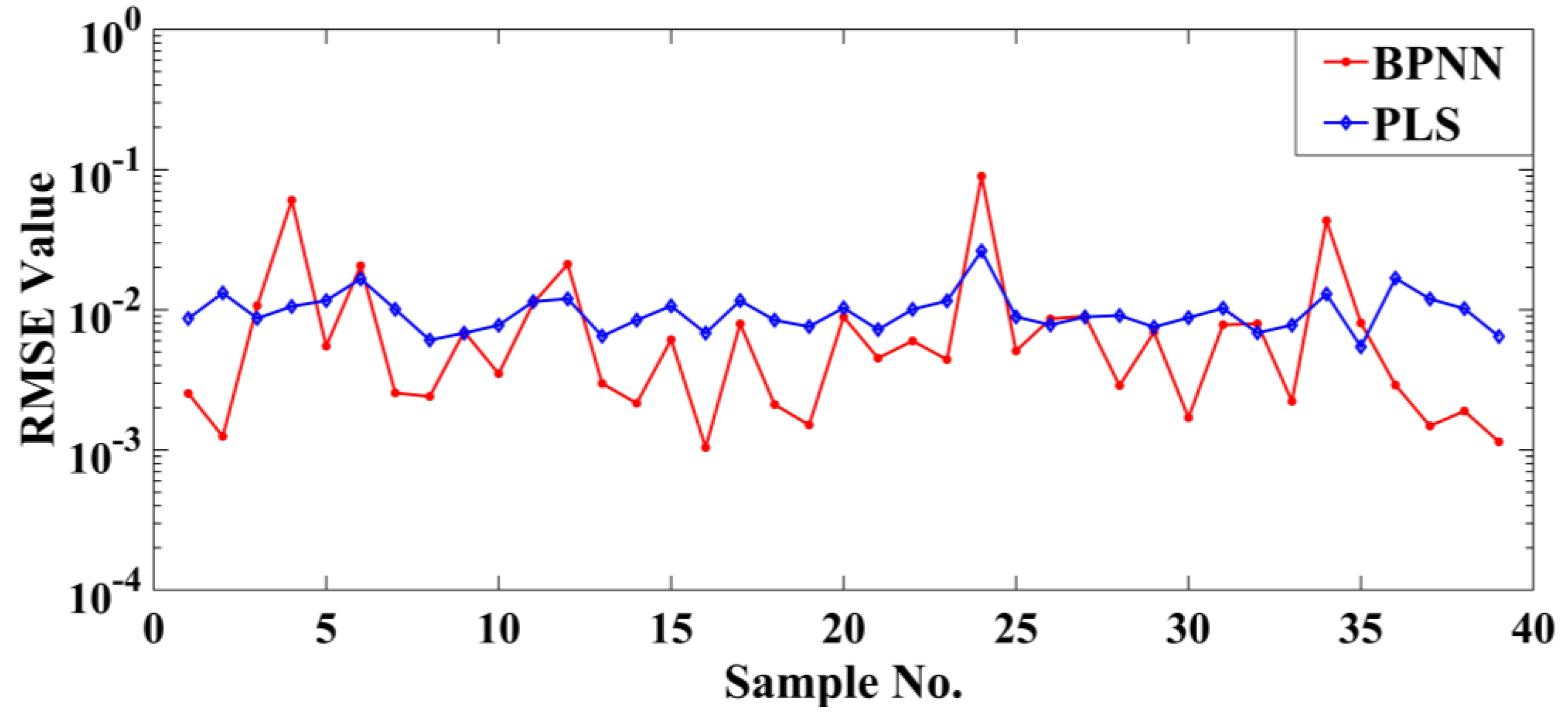
3.1.1. Analysis of Original Spectra Set

Figure 5 shows the relationship between the RMSE and validation sample number of the original spectra. One can compare the analysis ability of the BPNN and PLS based on the figure. The red line with circle represents the analysis results of the BPNN, and the blue line represents the analysis results of the PLS. In order to show the differences between the data more clearly, the y-axis uses logarithmic coordinates. When selecting a different sample for verification, it can be seen that the RMSE values changed obviously.

It can be seen in Figure 5 that most samples could obtain lower RMSE values using the BPNN. The advantage of the PLS was stability, while the BPNN was more accurate. Only four samples (4, 12, 24, and 34) had significantly higher RMSE values than the PLS when using the BPNN for prediction. It can be seen in Table 5 that these four samples had higher RE values than the PLS when using the BPNN for prediction. In Table 3, it can be seen that the concentrations of Sample Nos. 4, 12, and 24 were the highest for all samples, and all three of them were more than 10%. Therefore, we speculated that the accuracy of the PLS was better than that of the BPNN when predicting samples with a higher concentration. For all samples with a concentration less than 1% among the 39 samples, the RMSE values of the BPNN-predicted results were less than those of the PLS, and the lowest RMSE value of 0.0010 appeared when predicting sample 16. The RMSE value of Sample No. 2, which had the lowest MgO concentration (0.057%), was only 0.0012. In general, the BPNN could obtain better results than the PLS in predicting samples with lower concentrations in this experiment.

When comparing the RE values of the two chemometrics methods using the original spectra, it can be seen that Sample Nos. 2, 7, and 33 with low concentrations had the largest RE values when using the PLS to analyze. The MgO concentration of these samples was lower than 0.1%. When the PLS was used to predict the samples with a high concentration, relatively lower RE values could be obtained compared with the BPNN. In order to show the prediction accuracy of the BPNN and PLS more intuitively, we arranged the concentrations of 39 samples in ascending order and compared the AE of each sample obtained using two chemometrics methods. It can be seen that the AE values of the BPNN in predicting samples with a low concentration were smaller than those of the PLS (Figure 6). The AE values of the PLS prediction were smaller for the samples with a high concentration, and the prediction results of the PLS were relatively stable. Based on this phenomenon, we speculated that the accuracy of the BPNN was higher and the prediction error is smaller when predicting samples with a lower concentration. The PLS was more stable than the BPNN, and the PLS showed better performance in predicting samples with a higher concentration.

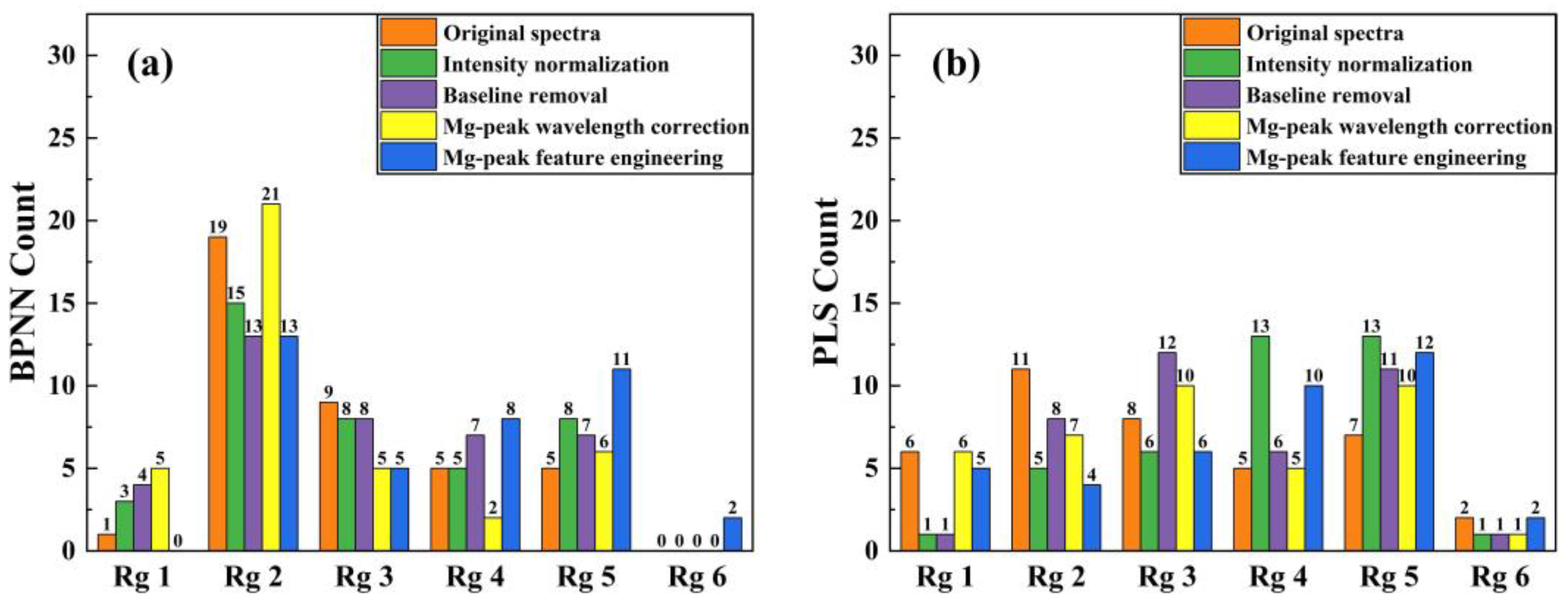
3.1.2. Analysis of Preprocessed Spectra Sets

In addition to the direct comparison of RMSE values, the statistical data of the results obtained under five types of spectra and different data sets are given in Table 4, including the maximum, minimum, average, and median of each method. The maximum value of the BPNN was larger than that of the PLS, and the minimum value was less than that of the PLS in all cases. When the difference between the averages was close, the median of the BPNN was smaller. Although most of the BPNN values were lower than those of the PLS for the same sample, the average values of the two chemometrics methods were not very different due to the large individual values. Taking this factor into account, we speculated that the prediction ability of the BPNN was better than that of the PLS.

When using Sample Set 1 to conduct the quantitative analysis, two chemometrics methods were employed to analyze five sets of spectra; i.e., the original spectra set and the first four preprocessed spectra sets (the concentration range reduction spectra set results are displayed individually in Section 3.1.3). Hence, each target sample could correspond to a total of 10 schemes when it was used as the testing sample (5 schemes for PLS and 5 schemes for BPNN).

For each scheme, we counted the number of samples on which this scheme could achieve the minimum RMSE value among the 10 schemes. The statistical results are shown in Figure 7. It can be seen that there were 34 samples with the minimum RMSE obtained by the BPNN, and this number was significantly more than 5 samples obtained by the PLS. Moreover, the scheme of “BPNN + Mg-peak wavelength correction preprocessing” had the highest accuracy on as many as 11 samples, which was the most among all 10 schemes. To verify whether the Mg-peak wavelength corrected spectra could obtain more accurate results when using the BPNN, the RE values were also examined.

For the BPNN method, the lowest RMSE value was obtained when Sample No. 14 was the testing sample and the Mg-peak wavelength corrected spectra set was used (the RMSE was 0.0007). The RE value obtained in the case was also the lowest compared with other schemes. For the BPNN method, the RMSE value obtained on the original spectra was 0.18 and the corresponding RE value was 60.74%, while the RMSE value on the Mg-peak corrected spectra was 0.0007 and the corresponding RE value was 20.53%. For the PLS method, when using the original spectra, the RMSE value was 0.0084 and the corresponding RE value was 219.96%. The RE values of the BPNN were far less than those of the PLS. It can be seen in Table 6 that when the Mg-peak wavelength corrected spectra were used, the average RE of the BPNN was 50.2%, which was the smallest RE value among the five sets of spectra when using the BPNN. In addition, the PLS counterpart was 142.29%, also the smallest among the five sets of spectra when using the PLS.

When the PLS was used for quantitative analysis, all of the average RE values exceeded 100%. However, if the BPNN was employed, the average RE values would exceed 100% only when the Mg-peak feature engineering was used as the preprocessing. The advantage of a BPNN is that one may improve the performance through the optimization of the various parameters so that excessive RE values can often be avoided by parameter adjustment. By contrast, the adjustable space of the PLS model is much smaller, leading to the occurrence of extremely large RE values (over 1000%). A BPNN requires a large amount of data to establish a good model. Therefore, when only two Mg-peak feature values were adopted as the input of the BPNN, too little information could be learned, and the performance of BPNN was poor no matter how we adjusted the parameters.

It is worth mentioning that for both the PLS and BPNN, the lowest level of the RE could reach a 0.1% order of magnitude only when the Mg-peak wavelength corrected spectra were used for analysis. For the BPNN, the minimum RE value was lower than 1% except for the Mg-peak feature scheme. This proved that good prediction results could be obtained when using the BPNN for quantitative analysis. In addition, when the Mg-peak wavelength corrected spectra were used, the maximum RE was also smaller than for other spectra.

In order to go a step further in the comparison of the RE values, six RE value ranges were set to characterize different accuracy levels. These six RE ranges were (0, 10], (10, 30], (30, 50], (50, 100], (100, 1000] and (1000, +∞), respectively (RE values in %), which are denoted as Rg 1 to Rg 6 for simplicity. The distribution results are shown in Figure 8. It can be seen that there were 94 RE values of the BPNN falling in Rg 1 and Rg 2, and the number for the PLS was 54. A large number of RE values of the PLS fell in Rg 4, Rg 5, and Rg 6, indicating the relatively low accuracy of the PLS quantification.

For the BPNN, there was no case in which the greatest RE value exceeded 1000% for the four approaches using full spectral information. Among these four spectra, using the Mg-peak wavelength corrected spectra could obtain the best overall accuracy. Not only were the RE values falling in ranges 1 and 2 more than when using other spectra, but the number of samples that had RE values less than 30% was 26, significantly more than for other spectra. When using the Mg-peak corrected spectra, five samples could achieve very high accuracy (i.e., with RE values falling in Rg 1), more than for the other kinds of spectra.

The above results indicated that higher accuracy could be obtained when using the Mg-peak wavelength corrected spectra with the BPNN in this work. It is also worth noting that when the Mg-peak feature was used to analyze, the number of RE values greater than 30% was also more than for the others, and there was no RE value less than 10%. For the other spectra, the accuracy of prediction did not differ much, and the phenomenon was not worth analyzing.

As for the PLS method, the number of RE values falling in Rg 1 was a bit larger than that of the BPNN, but the number of RE values falling in Rg 1 and Rg 2 was apparently lower than that of the BPNN. Moreover, all sets of spectra had RE values falling in Rg 6, indicating a lower predication ability of the PLS model herein. In addition, unlike the BPNN case, using the Mg-peak feature engineering scheme did not obviously decrease the overall accuracy. This was in line with expectations because PLS is a classical statistical method instead of a big-data-required machine learning method. This result also implied that the intensity values of the two prominent Mg peaks played a major role in the PLS calculation.

The overall RE values of all the 39 samples indicated that more accurate results could be achieved if the Mg-peak wavelength corrected spectra set was utilized regardless of whether the BPNN or PLS method was employed.

When the intensity-normalized and baseline-removed spectra were used for analysis, the prediction accuracy was not significantly improved. For the PLS, these two spectral preprocessing approaches improved the accuracy of the prediction results if we considered the statistics of the RE. It may be that the preprocessing approaches were helpful in the extraction of the Mg peaks, making the analysis results more accurate. For the BPNN, intensity normalization had no significant impact, and the result for the normalized spectra was close to the result of the original spectra. In the samples analyzed this time, the performance of BPNN was decreased due to removing the baseline of spectra. Considering that a BPNN is a non-linear machine learning method, other elements could affect the Mg-peak strength. The baseline may have contained information that was conducive to its learning, so the impact of the baseline removal on the quantitative analysis is still uncertain.

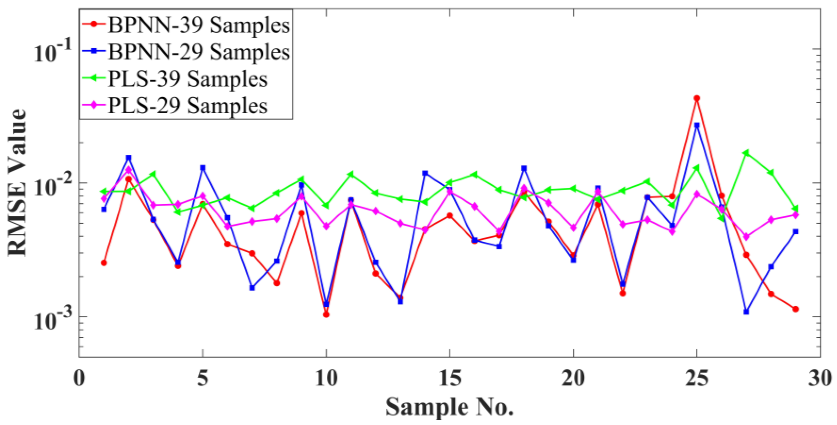
3.1.3. Analysis of Concentration Range Reduction Spectra Set

In addition to the above four preprocessing approaches, we also examined the influence of the sample set size on the quantification accuracy by utilizing a concentration range reduction preprocessing scheme. The MgO concentration range was 0.12–2.98% for the 29 samples in Sample Set 2. The analytical results for the samples that existed in both samples sets are displayed. The RMSE results are exhibited in Figure 9, and specific RE values are shown in

Table 7. The RE values (in %) of the 29 samples in Sample Set 2 and the quantitative analysis results of those samples in Sample Set 1 are displayed. The last row shows the average number of each column.

Sample No.	BPNN Set 1	BPNN Set 2	PLS Set 1	PLS Set 2
1	22.59	91.51	66.87	57.84
2	93.11	197.52	54.78	156.66
3	45.53	30.68	103.29	29.00
4	24.08	43.51	7.09	45.77
5	63.64	99.07	20.08	62.00
6	28.50	13.53	24.79	12.64
7	32.24	12.85	25.79	24.34
8	18.88	49.42	57.19	27.06
9	45.25	109.86	110.10	60.24
10	11.35	12.90	13.82	18.93
11	57.52	48.47	105.49	32.77
12	28.51	15.77	28.32	35.22
13	11.61	10.23	8.89	19.07
14	35.35	27.72	3.73	11.91
15	49.67	114.91	98.70	69.47
16	51.16	236.78	129.89	41.43
17	35.38	23.42	67.67	13.66
18	68.39	184.50	51.47	80.13
19	121.27	17.52	35.79	40.16
20	25.04	16.78	61.36	16.59
21	56.71	102.45	6.64	68.32
22	13.60	7.84	59.09	12.86
23	91.33	47.27	99.82	16.84
24	82.13	34.59	35.47	9.54
25	427.48	52.82	162.62	64.54
26	76.29	59.56	12.05	38.20
27	158.59	66.48	274.49	7.62
28	22.28	21.32	112.14	10.61
29	10.56	40.97	21.70	31.04
Average	62.34	61.73	64.11	38.43

.

After the concentration range of the training set was reduced, the accuracy of the PLS was significantly improved, and both the RMSE and RE were the best. As can be seen in Figure 9, when using Sample Set 2 for analysis, the RMSE values of almost all samples were lower than those of Sample Set 1. Based on the RMSE statistical data given in Table 4, it can be seen that the average of the RMSE was only 0.0064 when Sample Set 2 was used for the quantitative analysis. In this experiment, after reducing the sample concentration, the performance of the PLS was significantly improved, the prediction range was more accurate, and the average of the RE was only 39. We speculated that the concentration range of the sample set had a great impact on the final results for the linear method.

For the BPNN, the change in the sample set had little impact on the accuracy of the analysis results, and there was no obvious improvement in the prediction accuracy. The average of the RE did not decrease significantly, and the prediction results of some samples were actually worse than those for Sample Set 1. When using the BPNN for content prediction, the larger the number of samples, the higher the accuracy of the final prediction results. The concentration range of samples in this experiment had little influence on the final results because the change in sample set concentration had no significant impact on the results of the BPNN. Therefore, it can be indicated that as the training set expanded, the concentration range of the samples became larger, and the results obtained by BPNN would be more accurate.

3.2. Discussion

In addition to the results analyzed in Section 3.1, several additional details that might be important are discussed herein.

3.2.1. The BPNN Parameters

One of the most important parameters of the three-layer BPNN model is the number of hidden layer neurons. According to the parameter testing on the LIBS dataset in our previous studies, we found that 1024 was a good number for the hidden neuron parameter. Therefore, in the current work we inherited this number; i.e., 1024. It should be noted that a simple test was performed before we confirmed that 1024 was still a good enough value for the LIBS data in this study.

Specifically, 2 of the 39 samples were randomly selected as the testing sample, and the effect of hidden neuron number was investigated based on their original spectra. The two chosen samples were Sample No. 1 and Sample No. 4, and we tried 100, 500, 1024, and 2000 neurons. For Sample No. 1, the testing RMSE values were 0.1012, 0.0078, 0.0025 and 0.004, respectively. For Sample No. 4, the testing RMSE values were 0.1086, 0.0737, 0.0605 and 0.0743, respectively. Apparently, the parameter value of 1024 could outperform the other three parameter values in terms of the testing accuracy. Despite the fact we did not implement a thorough investigation based on all the samples, these results indicated that 1024 is a credible parameter value for the BPNN model in the current work.

Another important parameter was the number of iteration steps for the BPNN model training. In this work, the iteration number was set to be 801. Figure 10 shows the RMSE vs. step curve when Sample No. 1 was adopted as the testing sample (the step range is from 101 to 801). It can be seen that when the number of iterations was 801, the RMSE value could converge to a small value. In very few cases (e.g., Sample No. 5), further increasing the iteration number could yield an even smaller RMSE value. However, the improvement was very tiny, so we still adopted the results of the 801-step scheme.

It is worth mentioning that although the RMSE value tended to decrease in a relatively smooth pattern, the changing trend of the loss function value was very different. The loss vs. step curve when Sample No. 1 was adopted as the testing sample is shown in Figure 11. As can be seen in Figure 11a, the loss function value dropped sharply in the first 20 steps, while in Figure 11b one can find that it kept oscillating at a certain level during the latter part of the training process.

3.2.2. The Overfitting Check

One of the most notorious shortcomings of neural network algorithms is the overfitting problem. The overall accuracy of the training set is a key factor used to analyze whether overfitting appears in the training. Here, the BPNN model trained when Sample No. 1 was used as testing sample is taken as the example to demonstrate the condition of overfitting in this study. When Sample No. 1 was used as the testing set sample, the BPNN model was trained by the spectra from the other 38 samples (i.e., Sample No. 2 to Sample No. 39).

Figure 12 displays the RMSE values of the 39 samples when Sample No. 1 was in the testing set and Sample No. 2 to Sample No. 39 were in the training set. The RMSE of the testing sample was 0.0025 (red square). It can be seen that some of the training samples had lower RMSE values, while some of the training samples had higher RMSE values (blue dots). Generally, the overall RMSE level of the training samples was approximately the same as the RMSE value of the testing sample. Based on this example, one may infer that there was no apparent overfitting or underfitting phenomenon for the BPNN model in this work.

3.2.3. Some other Chemometrics Methods

Based on the analysis in the previous sections, one may find that some specific spectral preprocessing schemes have the potential to improve the performance of LIBS chemometrics; e.g., the Mg-peak wavelength correction approach.

In order to investigate whether this spectral preprocessing approach could improve the accuracy of other chemometrics algorithms, we applied two additional algorithms, namely OLS and ENet, to the original spectra set and the Mg-peak wavelength correction spectra set.

The RMSE values of the results predicted by the OLS and the ENet are shown in Figure 13. For the ENet, 23 samples could obtain a smaller RMSE after using Mg-peak wavelength corrected spectra. For the OLS, the minimum value of the RE was 5.34 and the maximum value was 1599 when using Mg-peak wavelength corrected spectra. For the original spectra, the minimum RE value was 13.26 and the maximum RE value was 2925. This spectral preprocessing approach had a similar effect on the OLS as the PLS, with both the maximum and minimum values decreasing.

To further compare the RE values, five RE ranges were set to represent different accuracy levels, namely (0, 30], (30, 50], (50, 100], (100, 1000] and (1000, +∞), respectively (RE values in %). The distribution results are shown in Figure 14. For the ENet, the quantification accuracy of the Mg-peak wavelength corrected spectra was generally higher than that of the original spectra, as can be inferred from the counts in Rg 1 and Rg 2. This result further confirmed that the Mg-peak wavelength correction was beneficial to accuracy improvement for the ENet method. For the OLS, there was hardly any positive information that could support the benefit of Mg-peak correction preprocessing based on the counts in Figure 14. Combined with the positive information provided in Figure 13, it may be concluded that the effect of Mg-peak correction on the OLS method was ambiguous and needs further investigation. Hence, from the comprehensive results of the BPNN, PLS, and ENet, it was shown that the Mg-peak wavelength correction preprocessing scheme really has great potential to improve the accuracy of MgO component quantification.

More calculations based on other algorithms, whether regular machine learning methods (e.g., Ridge and RF [20]) or sophisticated deep learning methods (e.g., convolutional neural networks [19]), will be carried out in our future work so that the effect of specific spectral preprocessing schemes can be further revealed.

4. Conclusions

In this study, we collected more than 2300 LIBS spectra from 39 geochemical samples using a MarSCoDe laboratory model in a simulated Martian atmospheric environment. Two LIBS chemometrics methods; i.e., PLS and BPNN, were employed to quantify the MgO concentration in the 39 samples. The results indicated that the BPNN model was better than the PLS model in terms of overall accuracy, especially for those samples with a relatively low MgO concentration. The PLS model could show better performance in the prediction of those samples with a high MgO concentration, and the PLS results were more stable than the BPNN results. For the two chemometrics methods, more accurate analysis results could be achieved when using the Mg-peak wavelength corrected spectra, as indicated by the RMSE and the RE values.

For the PLS, the employment of a sample set with a reduced concentration range could significantly improve the quantification accuracy. Intensity normalization and baseline removal could slightly improve the accuracy, while Mg-peak feature engineering hardly had any effect on accuracy promotion.

For the BPNN, the effect of either intensity normalization or baseline removal could be definitely determined and needs further examination. Mg-peak feature engineering would greatly reduce the accuracy because two Mg-peak intensity values can provide the BPNN model with too little information for its learning.

The Mg-peak wavelength correction was the most shining preprocessing scheme in this study, bringing clear benefits to the MgO quantification accuracy improvement for both the BPNN and PLS. In addition, this preprocessing approach also showed good performance in the ENet method. These results indicated that wavelength correction based on a certain element has great potential in promoting the accuracy of quantifying the content of the element.

Despite the fact that the sample set size was not too large, this study put forward new ideas for improving the accuracy of LIBS quantification. Larger sample datasets will be adopted in our future work to further investigate the effects of the specific spectral preprocessing schemes.

References

1. Wu, X.; Liu, Y.; Zhang, C.; Wu, Y.; Zhang, F.; Du, J.; Liu, Z.; Xing, Y.; Xu, R.; He, Z.; et al. Geological Characteristics of China’s Tianwen-1 Landing Site at Utopia Planitia, Mars. Icarus 2021, 370, 114657. [Google Scholar] [CrossRef]
2. Xu, W.; Liu, X.; Yan, Z.; Li, L.; Zhang, Z.; Kuang, Y.; Jiang, H.; Yu, H.; Yang, F.; Liu, C.; et al. The MarSCoDe Instrument Suite on the Mars Rover of China’s Tianwen-1 Mission. Space Sci. Rev. 2021, 217, 64. [Google Scholar] [CrossRef]
3. Zou, Y.; Zhu, Y.; Bai, Y.; Wang, L.; Jia, Y.; Shen, W.; Fan, Y.; Liu, Y.; Wang, C.; Zhang, A.; et al. Scientific Objectives and Payloads of Tianwen-1, China’s First Mars Exploration Mission. Adv. Space Res. 2021, 67, 812–823. [Google Scholar] [CrossRef]
4. Khajehzadeh, N.; Haavisto, O.; Koresaar, L. On-Stream and Quantitative Mineral Identification of Tailing Slurries Using LIBS Technique. Miner. Eng. 2016, 98, 101–109. [Google Scholar] [CrossRef]
5. Harmon, R.S.; Remus, J.; McMillan, N.J.; McManus, C.; Collins, L.; Gottfried, J.L.; DeLucia, F.C.; Miziolek, A.W. LIBS Analysis of Geomaterials: Geochemical Fingerprinting for the Rapid Analysis and Discrimination of Minerals. Appl. Geochem. 2009, 24, 1125–1141. [Google Scholar] [CrossRef]
6. Sobron, P.; Wang, A.; Sobron, F. Extraction of Compositional and Hydration Information of Sulfates from Laser-Induced Plasma Spectra Recorded under Mars Atmospheric Conditions–Implications for ChemCam Investigations on Curiosity Rover. Spectrochim. Acta Part B At. Spectrosc. 2012, 68, 1–16. [Google Scholar] [CrossRef]
7. Wiens, R.C.; Maurice, S.; Barraclough, B.; Saccoccio, M.; Barkley, W.C.; Bell, J.F.; Bender, S.; Bernardin, J.; Blaney, D.; Blank, J.; et al. The ChemCam Instrument Suite on the Mars Science Laboratory (MSL) Rover: Body Unit and Combined System Tests. Space Sci. Rev. 2012, 170, 167–227. [Google Scholar] [CrossRef]
8. Maurice, S.; Wiens, R.C.; Bernardi, P.; Caïs, P.; Robinson, S.; Nelson, T.; Gasnault, O.; Reess, J.M.; Deleuze, M.; Rull, F.; et al. The SuperCam Instrument Suite on the Mars 2020 Rover: Science Objectives and Mast-Unit Description. Space Sci. Rev. 2021, 217, 64. [Google Scholar] [CrossRef]
9. McLennan, S.M.; Anderson, R.B.; Bell, J.F.; Bridges, J.C.; Calef, F.; Campbell, J.L.; Clark, B.C.; Clegg, S.; Conrad, P.; Cousin, A.; et al. Elemental Geochemistry of Sedimentary Rocks at Yellowknife Bay, Gale Crater, Mars. Science 2014, 343, 1244734. [Google Scholar] [CrossRef] [Green Version]
10. Vaniman, D.T.; Bish, D.L.; Ming, D.W.; Bristow, T.F.; Morris, R.V.; Blake, D.F.; Chipera, S.J.; Morrison, S.M.; Treiman, A.H.; Rampe, E.B.; et al. Mineralogy of a Mudstone at Yellowknife Bay, Gale Crater, Mars. Science 2014, 343, 1243480. [Google Scholar] [CrossRef]
11. Wiens, R.C.; Udry, A.; Beyssac, O.; Quantin-Nataf, C.; Mangold, N.; Cousin, A.; Mandon, L.; Bosak, T.; Forni, O.; Mclennan, S.M.; et al. Compositionally and Density Stratified Igneous Terrain in Jezero Crater, Mars. Sci. Adv. 2022, 8, eabo3399. [Google Scholar] [CrossRef]
12. Liu, C.; Ling, Z.; Wu, Z.; Zhang, J.; Chen, J.; Fu, X.; Qiao, L.; Liu, P.; Li, B.; Zhang, L.; et al. Aqueous Alteration of the Vastitas Borealis Formation at the Tianwen-1 Landing Site. Commun. Earth Environ. 2022, 3, 280. [Google Scholar] [CrossRef]
13. Lepore, K.H.; Fassett, C.I.; Breves, E.A.; Byrne, S.; Giguere, S.; Boucher, T.; Rhodes, J.M.; Vollinger, M.; Anderson, C.H.; Murray, R.W.; et al. Matrix Effects in Quantitative Analysis of Laser-Induced Breakdown Spectroscopy (LIBS) of Rock Powders Doped with Cr, Mn, Ni, Zn, and Co. Appl. Spectrosc. 2017, 71, 600–626. [Google Scholar] [CrossRef]
14. Yang, Y.; Hao, X.; Ren, L. Correction of Self-Absorption Effect in Calibration-Free Laser-Induced Breakdown Spectroscopy (CF-LIBS) by Considering Plasma Temperature and Electron Density. Optik 2020, 208, 163702. [Google Scholar] [CrossRef]
15. Li, J.; Lu, J.; Lin, Z.; Gong, S.; Xie, C.; Chang, L.; Yang, L.; Li, P. Effects of Experimental Parameters on Elemental Analysis of Coal by Laser-Induced Breakdown Spectroscopy. Opt. Laser Technol. 2009, 41, 907–913. [Google Scholar] [CrossRef]
16. Ewusi-Annan, E.; Delapp, D.M.; Wiens, R.C.; Melikechi, N. Automatic Preprocessing of Laser-Induced Breakdown Spectra Using Partial Least Squares Regression and Feed-Forward Artificial Neural Network: Applications to Earth and Mars Data. Spectrochim. Acta Part B At. Spectrosc. 2020, 171, 105930. [Google Scholar] [CrossRef]
17. Pořízka, P.; Klus, J.; Képeš, E.; Prochazka, D.; Hahn, D.W.; Kaiser, J. On the Utilization of Principal Component Analysis in Laser-Induced Breakdown Spectroscopy Data Analysis, a Review. Spectrochim. Acta Part B At. Spectrosc. 2018, 148, 65–82. [Google Scholar] [CrossRef]
18. Li, L.N.; Liu, X.F.; Yang, F.; Xu, W.M.; Wang, J.Y.; Shu, R. A Review of Artificial Neural Network Based Chemometrics Applied in Laser-Induced Breakdown Spectroscopy Analysis. Spectrochim. Acta Part B At. Spectrosc. 2021, 180, 106183. [Google Scholar] [CrossRef]
19. Li, L.N.; Liu, X.F.; Xu, W.M.; Wang, J.Y.; Shu, R. A Laser-Induced Breakdown Spectroscopy Multi-Component Quantitative Analytical Method Based on a Deep Convolutional Neural Network. Spectrochim. Acta Part B At. Spectrosc. 2020, 169, 105850. [Google Scholar] [CrossRef]
20. Anderson, R.B.; Forni, O.; Cousin, A.; Wiens, R.C.; Clegg, S.M.; Frydenvang, J.; Gabriel, T.S.J.; Ollila, A.; Schröder, S.; Beyssac, O.; et al. Post-Landing Major Element Quantification Using SuperCam Laser Induced Breakdown Spectroscopy. Spectrochim. Acta Part B At. Spectrosc. 2022, 188, 106347. [Google Scholar] [CrossRef]
21. Gasda, P.J.; Anderson, R.B.; Cousin, A.; Forni, O.; Clegg, S.M.; Ollila, A.; Lanza, N.; Frydenvang, J.; Lamm, S.; Wiens, R.C.; et al. Quantification of Manganese for ChemCam Mars and Laboratory Spectra Using a Multivariate Model. Spectrochim. Acta Part B At. Spectrosc. 2021, 181, 106223. [Google Scholar] [CrossRef]
22. Zhang, P.; Zhou, T.; Xia, D.; Zhang, L. Quantitative Analysis Research of ChemCam-LIBS Spectral Data of Curiosity Rover. Infrared Laser Eng. 2022, 51, 9. [Google Scholar]
23. Cousin, A.; Forni, O.; Maurice, S.; Gasnault, O.; Fabre, C.; Sautter, V.; Wiens, R.C.; Mazoyer, J. Laser Induced Breakdown Spectroscopy Library for the Martian Environment. Spectrochim. Acta Part B At. Spectrosc. 2011, 66, 805–814. [Google Scholar] [CrossRef]
24. Sears, D.W.G.; Benoit, P.H.; Mckeever, S.W.S.; Banerjee, D.; Kral, T.; Stites, W.; Roe, L.; Jansma, P.; Mattioli, G. Investigation of Biological, Chemical and Physical Processes on and in Planetary Surfaces by Laboratory Simulation. Planet. Space Sci. 2002, 50, 821–828. [Google Scholar] [CrossRef]
25. Cui, Z.; Jia, L.; Li, L.; Liu, X.; Xu, W.; Shu, R.; Xu, X. A Laser-Induced Breakdown Spectroscopy Experiment Platform for High-Degree Simulation of MarSCoDe In Situ Detection on Mars. Remote Sens. 2022, 14, 1954. [Google Scholar] [CrossRef]
26. Ralchenko, Y.; Kramida, A. Development of NIST Atomic Databases and Online Tools. Atoms 2020, 8, 56. [Google Scholar] [CrossRef] [PubMed]
27. Jia, L.; Liu, X.; Xu, W.; Xu, X.; Li, L.; Cui, Z.; Liu, Z.; Shu, R. Initial Drift Correction and Spectral Calibration of MarSCoDe Laser-Induced Breakdown Spectroscopy on the Zhurong Rover. Remote Sens. 2022, 14, 5964. [Google Scholar] [CrossRef]
28. Jin, G.; Wu, Z.; Ling, Z.; Liu, C.; Liu, W.; Chen, W.; Zhang, L. A New Spectral Transformation Approach and Quantitative Analysis for MarSCoDe Laser-Induced Breakdown Spectroscopy (LIBS) Data. Remote Sens. 2022, 14, 3960. [Google Scholar] [CrossRef]
Figure 1. The operating principle of the LIBS system of MarSCoDe (a) and the schematic diagram of MarSDEEP (b). The relevant parameters of the simulated Martian atmospheric environment in the vacuum cabin are marked, and the positions of the MarSCoDe instrument and the detection samples inside MarSDEEP are indicated.
Remotesensing 15 03311 g001
Figure 2. Images of some samples employed in the experiment: (a) some target samples (in the form of pressed tablets), including soft clay (GBW03115), yellow-red soil (GBW07405(GSS-5)), lead ore type-I (GBW07235), stream sediment type-VII (GBW07311(GSD-11)), stream sediment type-I (GBW07309(GSD-9)), and latosol (GBW07407(GSS-7)); (b) the sample stage (with 16 sample holders) that could move along on the track inside the sample cabin.
Remotesensing 15 03311 g002
Figure 3. (a) An original spectrum of Sample No. 25 (randomly picked from the 60 original spectra). (b) The spectrum shown in (a) after baseline removal. The main elements corresponding to some prominent peaks are identified and marked.
Remotesensing 15 03311 g003
Figure 4. Principle and structure diagram of the BPNN model, which mainly included an input layer, a hidden layer and an output layer. The input variables x1, x2, …, xn denote the intensity values of each spectrum, where n is 4506 herein. The number of hidden layer neurons in this model was 1024. There was only one output neuron that yielded the predicted MgO concentration y.
Remotesensing 15 03311 g004
Figure 5. RMSE values of original spectra when we predicted MgO content using two different methods. The red line represents the BPNN, the blue line represents the PLS, and the x-axis number represents the verification set sample number.
Remotesensing 15 03311 g005
Figure 6. The AE values of the BPNN and PLS when using the original spectra for prediction. The sequence of samples is different from other figures (it is arranged according to the concentration). A logarithmic y-axis is employed for better visualization. Grey diamonds represent the results of the BPNN, and red circles represent those of the PLS.
Remotesensing 15 03311 g006
Figure 7. The number of samples on which a certain scheme could achieve the minimum RMSE value among the 10 schemes, with 5 schemes for the BPNN (left) and 5 schemes for the PLS (right). Different colors represent the 5 different spectra sets. The value marked above each bar indicates the exact count. Note that the sum of the 10 above-bar values is 39, corresponding to the sample quantity in Sample Set 1.
Remotesensing 15 03311 g007
Figure 8. The statistical results of the RE values obtained using different spectra. The six ranges are (0, 10], (10, 30], (30, 50], (50, 100], (100, 1000] and (1000, +∞), respectively (RE values in %). (a) Distribution of the BPNN; (b) distribution of the PLS. The value marked above each bar indicates the exact count falling within this range, and different colors represent different spectra.
Remotesensing 15 03311 g008
Figure 9. The RMSE values obtained for Sample Set 1 and Sample Set 2. The data for Sample Set 1 only retains the samples that were common with Sample Set 2.
Remotesensing 15 03311 g009
Figure 10. The RMSE vs. step curve when Sample No. 1 was adopted as the testing sample. The step range is from 101 to 801 for a better visualization effect.
Remotesensing 15 03311 g010
Figure 11. The loss vs. step curve when Sample No. 1 was adopted as the testing sample: (a) a global view of the whole range of 1 to 801 steps; (b) a local zoom-in view of the range of 21 to 801 steps.
Remotesensing 15 03311 g011
Figure 12. The RMSE values of the 39 samples when Sample No. 1 was in the testing set and Sample No. 2 to Sample No. 39 were in the training set. The RMSE value of Sample No. 1 is represented by the red square, while the RMSE values of the other 38 samples are represented by the blue dots.
Remotesensing 15 03311 g012
Figure 13. The RMSE values of the results predicted by the OLS and the ENet methods. Each method was applied to two spectra sets; i.e., the original spectra set and the Mg-peak correction spectra set.
Remotesensing 15 03311 g013
Figure 14. The statistical results of the RE values obtained for different spectra. The five ranges are (0, 30], (30, 50], (50, 100], (100, 1000] and (1000, +∞), respectively (RE values in %). The value marked above each bar indicates the exact count falling within this range, and different colors represent different spectra.
Remotesensing 15 03311 g014