Article

Passive 3D Imaging Method Based on Photonics Integrated Interference Computational Imaging System

1
Key Laboratory of Intelligent Infrared Perception, Chinese Academy of Sciences, Shanghai Institute of Technical Physics of Chinese Academy of Sciences, Shanghai 200083, China
2
University of Chinese Academy of Sciences, Beijing 100049, China
*
Author to whom correspondence should be addressed.
Remote Sens. 2023, 15(9), 2333; https://doi.org/10.3390/rs15092333
Submission received: 15 March 2023 / Revised: 21 April 2023 / Accepted: 26 April 2023 / Published: 28 April 2023
(This article belongs to the Special Issue Laser and Optical Remote Sensing for Planetary Exploration)

Abstract

:
Planetary, lunar, and deep space exploration has become the frontier of remote sensing science, and three-dimensional (3D) positioning imaging technology is an important part of lunar and deep space exploration. This paper presents a novel passive 3D imaging method based on the photonics integrated interference computational imaging system. This method uses a photonics integrated interference imaging system with a complex lens array. The midpoints of the interference baselines formed by these lenses are not completely overlapped. The distance between the optical axis and the two lenses of the interference baseline are not equal. The system is used to obtain the complex coherence factor of the object space at a limited working distance, and the image evaluation optimization algorithm is used to obtain the clear images and 3D information of the targets of interest. The simulation results show that this method is effective for the working scenes with targets located at single or multiple limited working distances. The sharpness evaluation function of the target presents a good unimodality near its actual distance. The experimental results of the interference of broad-spectrum light show that the theoretical basis of this method is feasible.

Graphical Abstract

1. Introduction

After decades of development, human beings have carried out space exploration activities on the moon, Mars, asteroids, and other celestial bodies. Planetary, lunar, and deep space exploration has become the frontier of scientific development. 3D imaging technology aims to obtain the 3D information of a target scene. It can provide support for the 3D mapping of celestial bodies, the positioning and navigation of the inspector, and the safe operation of the detector, which has significant research value. At this stage, vision-based 3D imaging technology is mainly divided into two categories: active and passive. Active methods include structured light [1,2,3] and lidar [4,5]. The structured light method introduces the active light sources to illuminate the target and obtains the 3D information of the target by calculating the change of light intensity or phase. It is mostly used for the 3D measurement of close-range targets. Zhang et al. reported 3D imaging of the face with an accuracy of 0.05 mm [3]. Lidar emits a pulse or continuous laser to the target and calculates the distance and azimuth parameters of the target by measuring the arrival time, strength, and other parameters of the reflected or scattered signal. Its working distance can reach very far. Li et al. used a single photon lidar to achieve active 3D imaging at a distance of 8.2 km with an accuracy of 5.5 cm [4], and achieved three-dimensional imaging at an absolute distance of 163.337 km with an accuracy of 3.5 cm [5]. These active 3D imaging methods have high accuracy and are insensitive to natural light and target texture. Passive methods mainly include the monocular estimation method [6], binocular or multi-view stereo vision method [7,8,9], and the oblique photography method [10,11]. The monocular estimation method calculates the 3D information of the target through the images of a single camera. Zhe et al. measured the vehicle target based on the principle of camera projection. The absolute error of the target in the range of more than 60 m is about 0.5 m [6]. The stereo vision method uses two or more cameras to capture the target at the same time and calculates the 3D information of the target based on the parallax principle. Its working range is from several meters to hundreds of meters. Wang et al. used the binocular method to perform 3D imaging of a target at a distance of 200 m, and the accuracy in the three coordinate axis directions was 0.28 m, 0.19 m, and 0.097 m, respectively [7]. Adil et al. located the target at 60~200 cm, and the highest positioning accuracy was 2.157 cm at 100 cm [8]. The oblique photography method uses a vertical camera and multiple oblique cameras to image the scene to obtain images of multiple angles at the same position, thereby reconstructing a 3D model. Xi et al. used an unmanned aerial vehicle (UAV) with a flight height of 200 m to carry out 3D reconstruction of the campus, and the ground point errors were 0.068 m, 0.055 m, and 0.093 m [10]. Qiu et al. used UAV oblique photography to perform 3D reconstruction of the waters. For scenes with a height of 38.5~53.3 m, the average error of 3D reconstruction was 0.303 m [11]. These passive 3D imaging methods do not require additional active light sources and have better concealment. Various 3D imaging methods have been proposed and have become a research hotspot in academic research.
The photonics integrated interference imaging system that combines the integrated photonics technology and the principle of interference imaging has been proposed in recent years [12,13,14]. Unlike traditional spatial domain diffraction imaging, this system uses thousands of paired lens arrays to collect light. It also uses photonic integrated circuit (PIC) chips placed behind the lens array to obtain a complex coherence factor related to the spatial frequency by interferometry. Then, it reconstructs the image of object space based on the interference results [15]. The system can significantly reduce the size, weight, and power compared to traditional telescopes [16], which makes it more convenient to install this system on UAV, airship, satellite, and other platforms for remote sensing or deep space exploration. The initial photonic integrated interference imaging system is designed as a radiation shape [13] which uses 37 radially arranged interference arms. Each interference arm consists of a linearly arranged lens array and a PIC chip under the lens. This system is vividly called the SPIDER imager. The imaging process of the photonic integrated interference imaging system is an under-sampling process of the target spatial frequency. Improving the coverage of the lens array to the spatial frequency spectrum is an effective method to improve the imaging quality of the system. Based on simulation, some studies have improved the frequency coverage by optimizing the lens matching method of the SPIDER imager [17,18], and some studies have improved the arrangement of lens arrays on the basis of radial arrangement. Representative studies include the second generation SPIDER system [16], hierarchical multistage sampling lens array [19], inhomogeneous multistage sampling lens array [20], odd–even alternating distribution array [21,22], and the hybrid architecture with small telescopes [18] or nested arrays [23] at the center of the array. Because the photonic integrated interference imaging system uses the waveguide array in PIC to form a combined field of view (FOV), the waveguide array placed behind each lens must have the same arrangement and direction. For the radial shape imager, if each interference arm uses the same PIC chip, the waveguide array on the PIC chip will rotate with the installation angle, resulting in waveguide arrays of different PIC chips facing different scenes. Therefore, the waveguide array on each PIC chip needs to be rotated differently according to its installation angle. Other studies no longer use radial shape layout, such as the hexagonal imager [24], the “chessboard” imager [25]. Another way to improve imaging quality is to use optimization algorithms in the computational imaging process, such as the image reconstruction algorithms based on improved entropy [26], compressed sensing [27], and deep learning [28]. Some research teams have designed and fabricated PIC chips with interferometer components and verified their interferometry capabilities [14,29,30,31]. In addition, based on the photonic integrated interference imaging system, we proposed a wide-field detection and tracking method by changing the interference baselines and the number of waveguides forming the combined FOV [32]. Liu et al. proposed a direction-finding system for point source targets with long distance and deviating from the optical axis based on silicon PIC chips and theories of interferometric imaging [31]. Numerous related studies have discussed the two-dimensional (2D) imaging results of the system under the assumption that the working distance is infinite, while ignoring the imaging capability of the system at a limited working distance. The term of complex coherence factor related to the depth dimension of the object space cannot be ignored when the photonics integrated interference imaging system is working at the limited working distance. This term affects the reconstruction of the image, but also brings a new research idea to the study of 3D imaging technology.
Based on the optical interference computational imaging theory, this paper discusses the conditions for reconstructing clear images based on a complex coherence factor collected by the photonics integrated interference imaging system at a limited working distance, which has been neglected by related research works. We found that the phase variation of the complex coherence factor caused by the midpoint configuration of the interference baselines, as well as the working distance, plays a decisive role in reconstructing clear images. Especially when the sub-field of view of the imaging where the midpoints of the interference baselines do not overlap is not much larger than the midpoint deviation of interference baselines, adjusting the introduced reference distance can significantly affect the sharpness of the target image. On this basis, we firstly propose a passive 3D spatial positioning imaging method based on the photonic integrated interference imaging system. In this method, the photonics integrated interference imaging system with a complex lens array is used to collect the complex coherence factor of the object space light at a limited working distance. The midpoints of the interference baselines formed by these lenses are not completely overlapped. The distance between the optical axis and the two lenses of the interference baseline are not equal. The image evaluation optimization algorithm is used to evaluate the quality of the reconstructed target image, varying with the reference distance step-by-step. The clear images and 3D information of the targets of interest are obtained simultaneously, which achieves the purpose of 3D positioning imaging.
Compared with the existing passive 3D imaging methods based on diffraction imaging technology, this method is based on the interferometry and computational imaging of the photonics integrated interference imaging system. It can obtain clear images and the 3D information of all targets with a single camera and single exposure. This paper is organized as follows: in Section 2, the influence of the interferometric baseline configuration and reference distance on the phase of complex coherence factor, as well as the sharpness of the reconstructed image at the limited working distance, are discussed, and the passive 3D imaging method is established. In Section 3, two simulation examples verify that this imaging method can obtain clear images and 3D information in single and multiple limited working distance target scenes. The interference experiment of the broad-spectrum light, based on the optical fiber system, verifies the relationship between the relative displacement of the spatial fringe and the midpoint of the interference baseline, the target distance, and the phase of the complex coherence factor, which indirectly verifies the correctness of the basic theory of the proposed method.

2. Materials and Methods

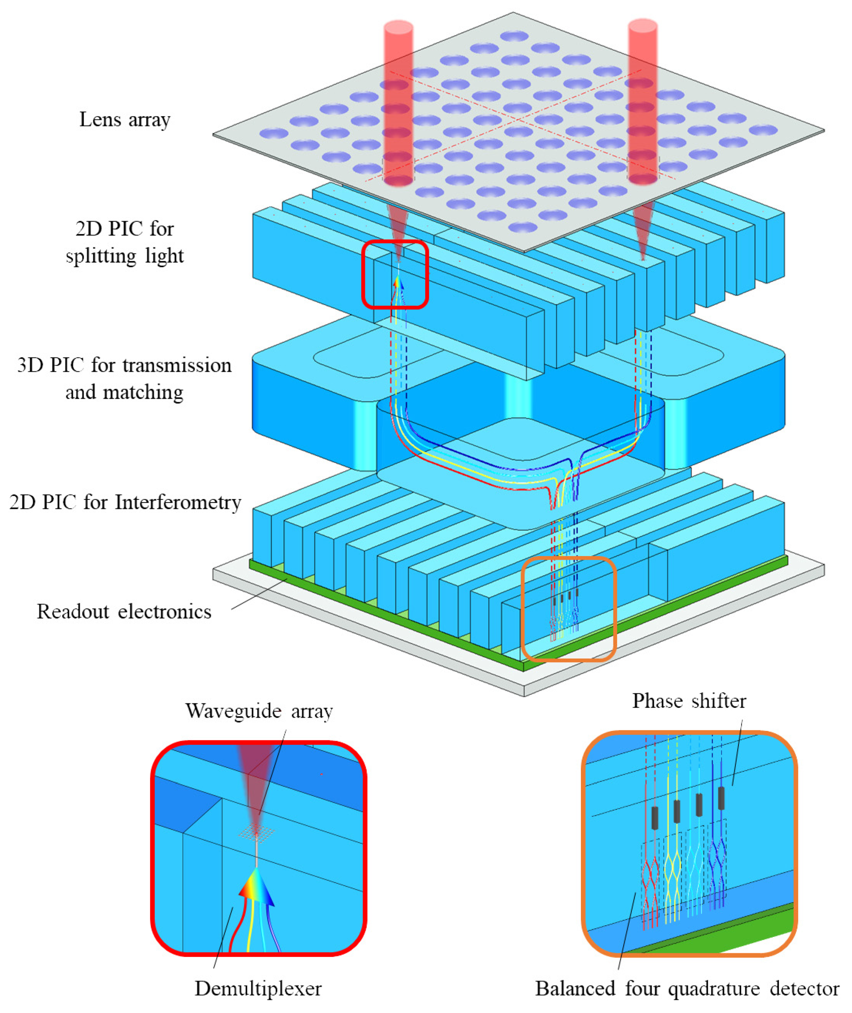
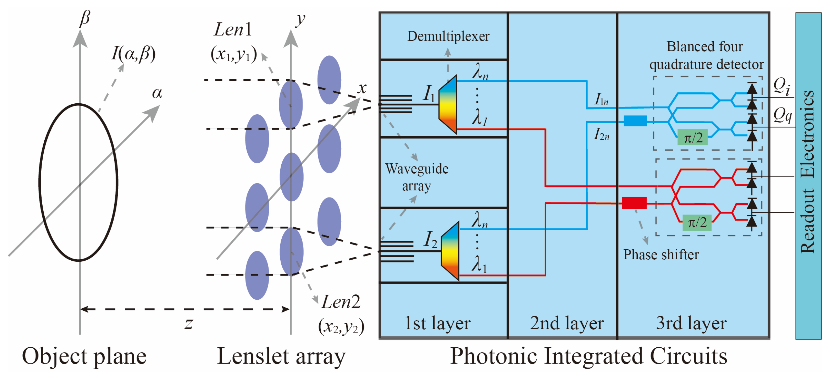
2.1. The Structure of a ‘Chessboard’ Photonic Integrated Interference Imager

The “checkerboard” imager shown in Figure 1 is a classic structure of the photonics integrated interference imaging system. The lens array of the “checkerboard” imager is set in a ( 2 N + 1 ) × ( 2 N + 1 ) square grid arrangement. These lenses are divided into four groups: N × N , N × ( N + 1 ) , ( N + 1 ) × N , and ( N + 1 ) × ( N + 1 ) . The lenses in each group are paired according to the central symmetry. This arrangement and pairing method can achieve uniform spatial frequency sampling in two orthogonal array directions and has better imaging results [25]. The imager uses three layers of PIC arrays. The first layer of 2D PIC after the lens array is designed with waveguide arrays and demultiplexers to split light. The second layer of 3D PIC is designed with phase shifters and balanced four quadrature detectors to transmit and match the light of each pair of lenses, bands, and sub-field. The third layer of 2D PIC is used for interferometry.
The 2D PICs with waveguide arrays in the “checkerboard” imager are parallel, so the rotation of the waveguide array required for the radial structure imager is avoided. It is only necessary to design and fabricate two PICs for the first layer, which are suitable for lens sequences with a length of N and N + 1 . The splitting and transmission of the hexagonal imager are completed by a 3DPIC [24], and its design and fabrication are difficult. Even if the system is designed to resemble the structure of three layer PICs in this paper, it is necessary to make 2D PICs with different lengths. The “checkerboard” imager has a more convenient design and manufacture than the radial imager and hexagonal imager. Therefore, the theoretical method of a passive 3D imaging scheme based on a photonics integrated interference computational imaging system is discussed according to the “checkerboard” image.

2.2. The Relationship between the Complex Coherence Factor Collected by the System and the Target Spatial Frequency, Distance and Working Parameters

The 2D schematic diagram of the imager is shown in Figure 2. Note that the coordinates of a pair of lenses forming an interference baseline on the plane of the lens array are ( x 1 , y 1 ) and ( x 2 , y 2 ) . The light from the sub-FOV I ( α , β ) collected by the two lenses are split by a demultiplexer. The matched beams with a center wavelength of λ n produce photocurrents Q i and Q q after orthogonal interference, and the value is [33]:
Q i = I 1 n I 2 n | γ ( τ ) | cos ψ
Q q = I 1 n I 2 n | γ ( τ ) | sin ψ
where | γ ( τ ) | is the mode of the complex degree of coherence of two beams, ψ is the phase of the complex degree of coherence of two beams, and I 1 n and I 2 n are the light intensity of two beams. Thus, the complex degree of coherence can be calculated as:
γ ( τ ) = c I 2 + Q 2 exp [ j arctan ( Q I ) ]
where c = 1 / I 1 n I 2 n . Since the lens array is adequately illuminated by the light source, it can be approximated that the beam intensity in the same spectral channel after each lens is equal [33]. Therefore, c is a constant, which can be calibrated by zero frequency sampling. τ is the optical path difference of the optical paths behind the two lenses. When two optical paths are equal by adjusting the phase shifter, the complex coherence factor μ is obtained:
μ = γ ( 0 )
which is the result of normalization of the mutual intensity J : μ = J / I 1 n I 2 n .
According to the Van Cittert–Zernike theorem, the mutual intensity of the collected light is [32]:
J ( x 1 , y 1 ; x 2 , y 2 ) = exp ( j φ ) ( λ ¯ z ) 2 I ( α , β ) × exp { j 2 π λ z ( Δ x α + Δ y β ) } d α d β
where λ ¯ is the working center wavelength, z is the target distance, I ( α , β ) is the light intensity distribution of the target, and Δ x = x 2 x 1 and Δ y = y 2 y 1 are the distance between the lens pair, which is the interference baseline B . The phase factor φ in the formula is [32]:
φ = π λ ¯ z [ ( x 2 2 + y 2 2 ) ( x 1 2 + y 1 2 ) ]
The spatial frequency domain collected by this lens pair is:
( u , v ) = 1 λ ¯ z ( Δ x , Δ y )
Therefore, the complex coherence factor can be expressed as:
μ ( x 1 , y 1 ; x 2 , y 2 ) = J ( x 1 , y 1 ; x 2 , y 2 ) [ I ( x 1 , y 1 ) I ( x 2 , y 2 ) ] 1 / 2 = exp [ j 2 π ( u x m + v y m ) ] [ I ( α , β ) ] | u , v I ( α , β ) d α d β
where x m = x 1 + x 2 2 and y m = y 1 + y 2 2 are the midpoint of the lens pair, and [ I ( α , β ) ] | u , v = I ( α , β ) × exp [ j 2 π ( u α + v β ) ] d α d β is the result of the 2D Fourier transform of I ( α , β ) about spatial frequency ( u , v ) . The phase of the complex coherence factor μ calculated from the signals collected by the lens pair consists of the phase of the spatial frequency of the target and an additional phase factor φ , which varies with the midpoint position ( x m , y m ) of the lens pair, working wavelength λ ¯ , and the target distance z .
The coordinate parameters of the lens pair and working wavelength are known. To discover the actual distance z of the target from phase factor φ , we apply a reference distance z c and a correction term μ c to the acquired signal. μ c consists of the coordinates of lens pair, working wavelength, and the set reference distance z c :
μ c = exp { j π λ ¯ z c [ ( x 2 2 + y 2 2 ) ( x 1 2 + y 1 2 ) ] }
Combining Formulas (6) and (7), the corrected signal is:
μ μ c = exp [ j 2 π ( u x m + v y m ) ( 1 z z c ) ] [ I ( α , β ) ] | u , v I ( α , β ) d α d β
The complex coherence factor with correction has a phase factor related to the actual distance z , the reference distance z c , working wavelength λ ¯ , and the baseline center position ( x m , y m ) .

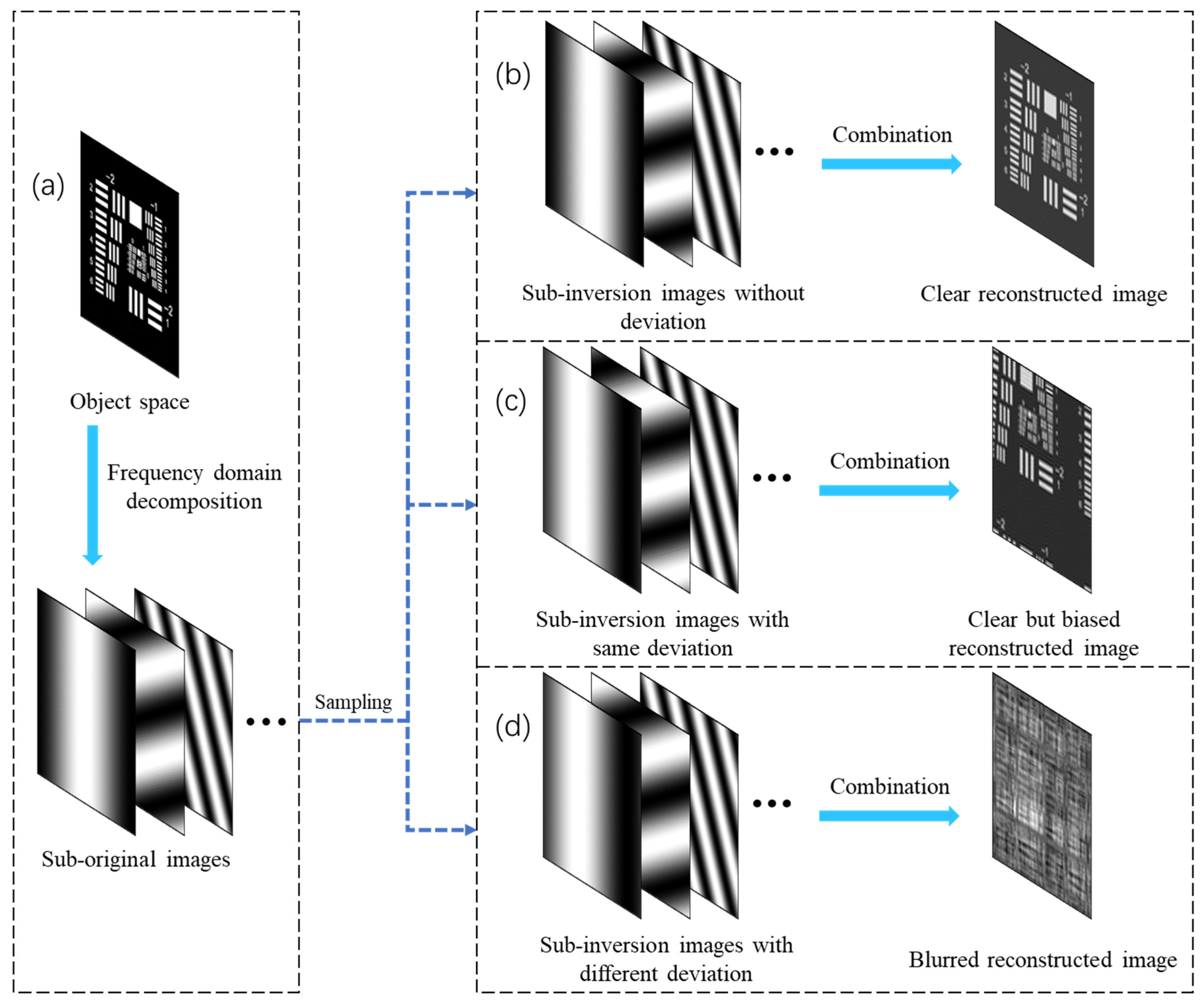
2.3. The Influence of the Phase of the Complex Coherence Factor on the Reconstructed Image

The photonics integrated interference imaging system performs discrete sampling of the spatial frequency through the acquisition signals of each interference baseline and reconstructs the image by the 2D inverse Fourier transform. For a single spatial frequency value with a frequency coordinate of ( u , v ) , the spatial domain image obtained by the 2D inverse Fourier transform is a set of sinusoidal fringes. We call it the sub-inversion image. The gray scale change direction of the stripe is: r = ( u , v ) = ( Δ x , Δ y ) . According to the linearity of the Fourier transform, the reconstructed image can be regarded as the superposition of the sub-inversion images obtained by the 2D inverse Fourier transform of the acquisition signal of each interference baseline. According to the displacement of the 2D Fourier transform, μ μ c [ I [ α + x m ( 1 z z c ) , β + y m ( 1 z z c ) ] ] | u , v , which is the result of the 2D Fourier transform of the object space with translation. Therefore, the phase change of the complex coherence factor causes the sub-inversion image corresponding to the spatial frequency ( u , v ) of this interference baseline to have a translation of s 0 , whose direction is r s = ( x m , y m ) . Considering the periodicity of the two-dimensional inverse Fourier transform, the translation of this interference baseline is:
s 0 = ( x m ( 1 z z c ) + a T x , y m ( 1 z z c ) + b T y )
where T x = 1 / u = λ ¯ z / Δ x and T y = 1 / v = λ ¯ z / Δ y are the period of sub-inversion image, and a and b are arbitrary integers.
As shown in Figure 3a, the object space can be regarded as the superposition of sinusoidal fringes after frequency domain decomposition. The imaging process of the imaging system is equivalent to the discrete sampling of these sinusoidal fringes; calculate the sub-inversion image with displacement and superimpose them to form a reconstructed image.
To measure the influence of the translation of the sub-inversion image on the reconstructed image, the image deviation, which is the ratio of the translation s 0 to the size of the reconstructed image, can be used. The size of the reconstructed image is the size of the FOV, which is calculated as L x = λ ¯ z / B min x , L y = λ ¯ z / B min y , where B min x and B min y are the shortest baseline in two orthogonal directions. Therefore, the image deviation of the sub-inversion image of this interference baseline is:
s = ( x m L x ( 1 z z c ) + a T x L x , y m L y ( 1 z z c ) + b T y L y )
The image deviation s decreases with the size of the FOV, and it increases with the midpoint deviation, which is the distance between the center of the interference baseline and the center of the optical axis. In addition, it is also related to the value of the reference distance z c . For different interference baseline configurations and reference distances, s have different values, and the corresponding sub-inversion images have different deviations. The value and dispersion of image deviations affect the sharpness of the reconstructed image.
If the coordinates of the midpoints of all interference baselines are equal to zero, such as the radial pairing method of the hexagonal imager [24], all image deviation s of the sub-inversion image can be zeros. Moreover, if the distance between the optical axis and two lenses of the interference baseline are equal, such as the lateral pairing method of the hexagonal imager [24], x 1 2 + y 1 2 = x 2 2 + y 2 2 , then r s r , which means the translation direction of the corresponding sinusoidal fringe is perpendicular to the gray change direction. The sub-inversion image is the same as the original sinusoidal fringe. Moreover, if the distance of the target is very far, the size of FOV will be much larger than the midpoint deviation. L x x m , L y y m , and all s will be close to ( a T x L x , b T y L y ) , which is equivalent to (0,0) according to the periodicity. In these cases, all sub-inversion images are in the correct position and the reconstructed image is clear, as shown in Figure 3b.
If the coordinates of the midpoints of each interference baseline are the same but not zero, all s can have the same value. All sub-inversion images have the same deviation, and the reconstructed image is clear but has deviation, as shown in Figure 3c. However, this situation does not occur for complex lens arrangements.
For an imager with an interference baseline configuration that does not meet the above conditions, it is possible to change the value and dispersion of image deviation s by adjusting the value of z c . When z c = z , 1 z z c = 0 and all s can take the same value ( a T x L x , b T y L y ) , which is equivalent to (0,0) according to the periodicity. The reconstructed image is currently clear. In addition, when z c is near z but z c z , all s are discrete. The image deviation of each inversion image is discrete, and the reconstructed image is blurred, such as when printing newspapers with misaligned colors, as shown in Figure 3d. Therefore, within the range near the actual distance z of target, the reconstructed image is clear only when z c = z . As z c moves away from z , the reconstructed image will become increasingly blurred. If the image evaluation function is used to evaluate the sharpness of reconstructed images with different z c values, a peak will appear near z .

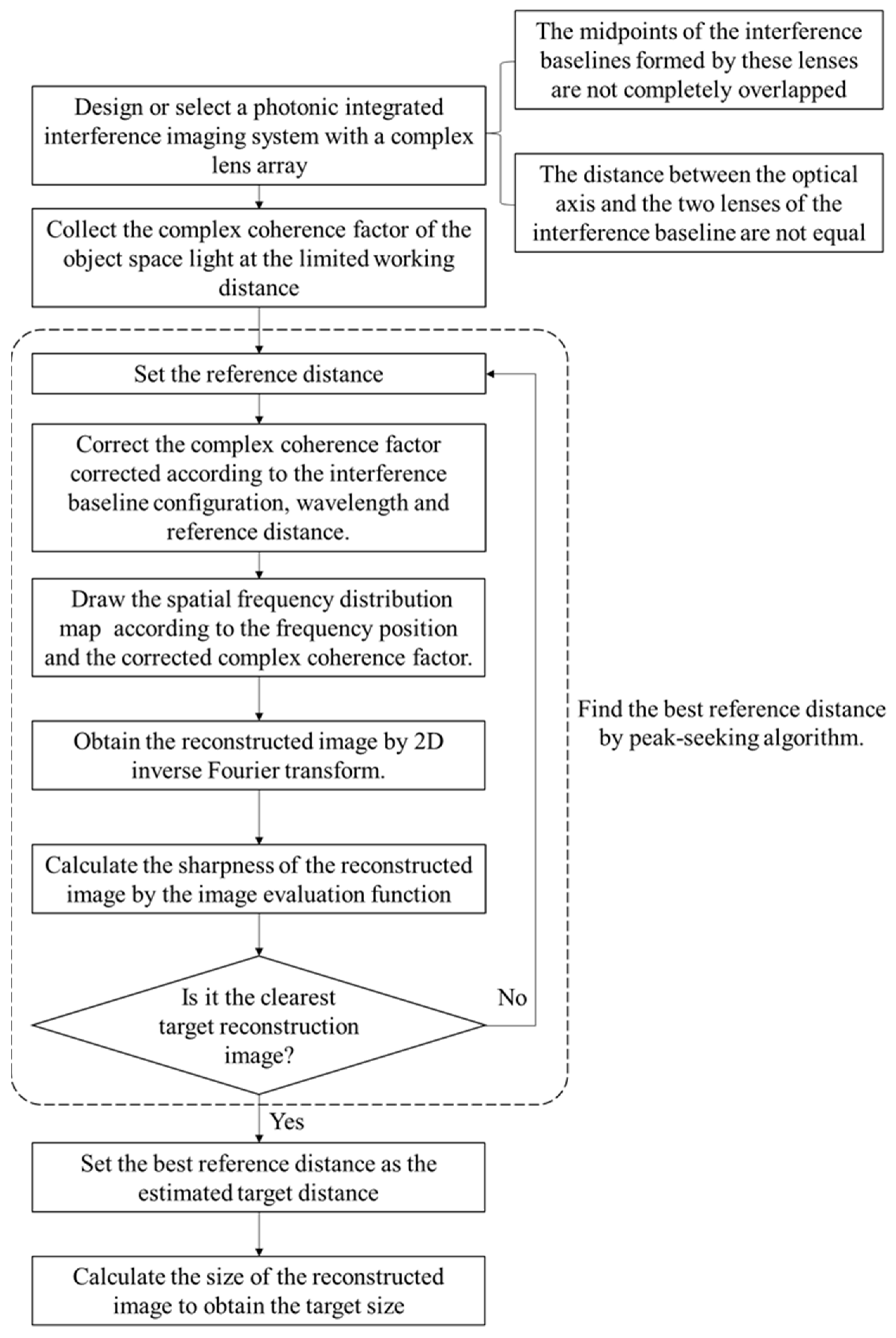
2.4. The Workflow of Three-Dimensional Positioning Imaging Method

According to the previous analysis, we can use a photonics integrated interference imaging system with a complex lens array to collect the complex coherence factor of the object space light at the limited working distance. The midpoints of the interference baselines formed by these lenses are not completely overlapped. The distance between the optical axis and the two lenses of the interference baseline are not equal. Thus, we use the image evaluation function to analyze the relationship between the sharpness of the target image and the reference distance. Next, we set the best reference distance to make the target reconstructed image clearest as the distance of target and calculate the size of the sub-FOV: L x c = λ ¯ z c / B min x , L y c = λ ¯ z c / B min y . We take them as the actual size of the reconstructed image and calculate the target size according to the relative position of the target in the reconstructed image. The size accuracy is positively related to the positioning accuracy of the distance. The working flow chart of the 3D positioning imaging is shown in Figure 4. This method is a passive visual 3D imaging method with a single camera and single exposure.

2.5. Performance Analysis

2.5.1. Working Range

The working range of the system is an important performance index. The target distance and the deviation between the midpoint of the interference baseline, as well as the optical axis, cause the phase changes of the complex coherence factor. To satisfy the interference theorem, the optical path changes corresponding to the phase changes cannot exceed the coherence length of the interference measurement, that is, λ ¯ φ / 2 π L c λ ¯ 2 / Δ λ . Δ λ is the bandwidth of each wavelength channel. According to Formula (6),
x m Δ x + y m Δ y z λ ¯ 2 Δ λ
The vector of the interference baseline length is expressed as B = ( Δ x , Δ y ) . The vector of the baseline midpoint coordinates is expressed as P m = ( x m , y m ) . Thus, x m Δ x + y m Δ y = B P m | B | | P m | = B d m . d m = x m 2 + y m 2 is the distance between the optical axis and midpoint of interference baseline. The value of x m Δ x + y m Δ y is the largest when the baseline direction is radial. Therefore, the minimum working distance of the system is:
z max ( B d m ) Δ λ λ ¯ 2 .
The far distance between the optical axis and the midpoint of the interference baseline, as well as the large working bandwidth, will limit the minimum working distance.
In addition, the uncorrected image deviation, which can be obtained by setting the reference distance to infinity, determines the sharpness of the reconstructed image without using the reference distance. According to Formula (12), the increase in the distance makes the image uncorrected deviation decrease until its influence can be ignored. To estimate the distance, the uncorrected image deviation | s | should be greater than κ . κ is the minimum value of image deviation when the displacement of the inversed image without correction makes the reconstructed image blurred, which can be estimated by simulation. According to Formula (12), | s | a has a minimum value d m / L , where L = λ ¯ z / B is the period corresponding to this interference baseline. Thus, the maximum working distance is calculated as:
z min ( B d m ) κ λ ¯
Reducing the working wavelength, increasing the length of the interference baseline, and increasing the distance between the midpoint of the baseline and the optical axis can improve the maximum working distance.

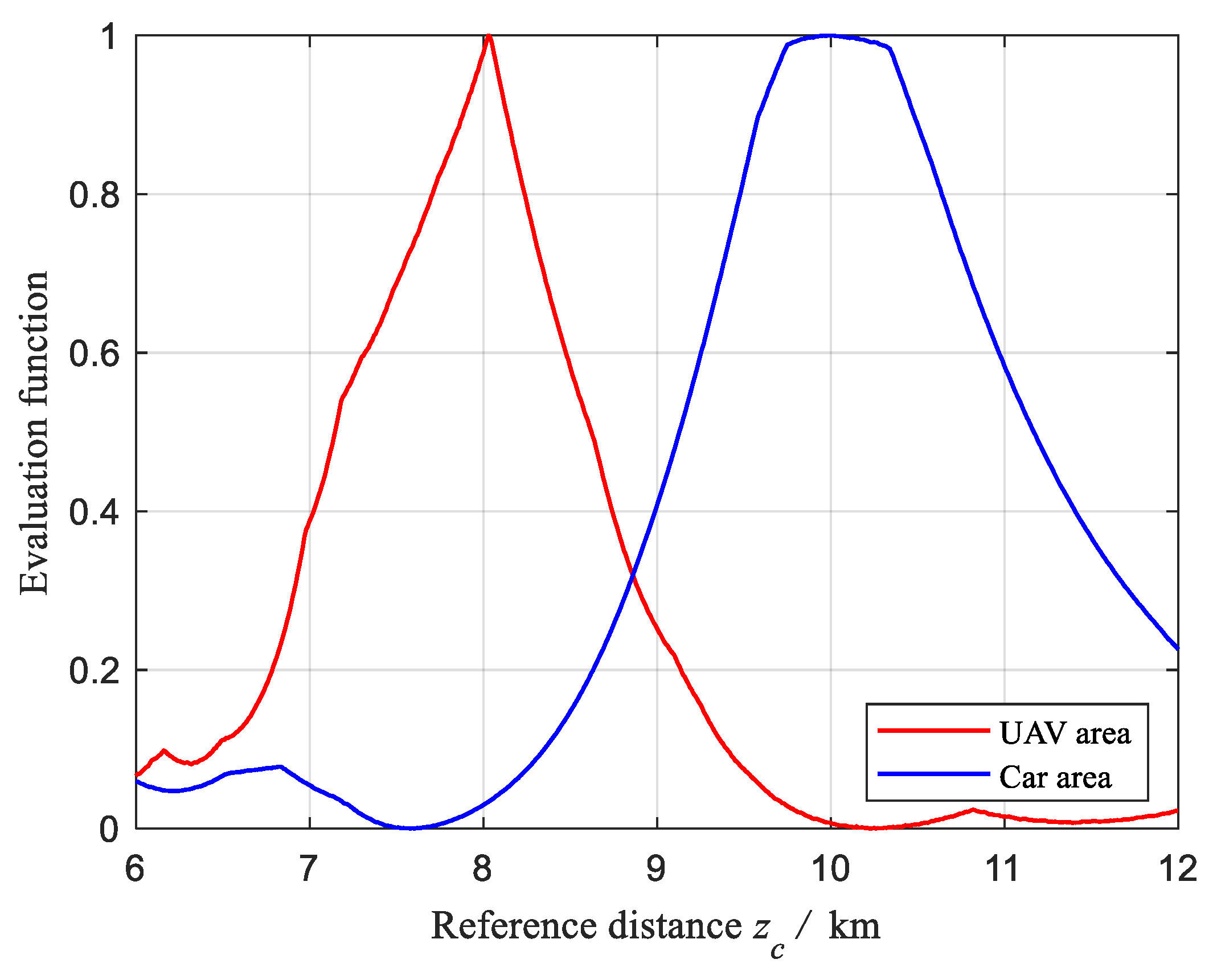
2.5.2. Influencing Factors of Positioning Accuracy

Positioning accuracy is an important indicator of 3D positioning imaging. The number and distribution of interference baselines in the photonic integrated interference imaging system directly determine the sampling range of the spatial frequency. More numbers and a more reasonable interference baseline configuration can obtain clearer optimal reconstructed images and a higher positioning accuracy. The blur of the reconstructed image is caused by the displacement of the sub-inversion image relative to the ideal fringe position. The process of finding the reference distance that makes the reconstructed image the clearest is the process of finding the reference distance that makes the image deviation zero. The larger and discrete image deviation makes the effect of adjusting the reference distance on the reconstructed image more significant, which helps to obtain a higher positioning accuracy. According to Formula (12), when the length and direction of the interference baseline are determined, increasing the distance between the midpoints of the interference baselines and the optical axis can increase the image deviation of the system, thus improving the positioning accuracy while ensuring the imaging quality.
The 3D positioning imaging method relies on the sharpness of the reconstructed image. The reconstructed image, when the reference distance is equal to the target distance, is called the best reconstructed image. The measurement errors of the complex coherence factor affect the spatial frequency value used for calculation and analysis, which in turn affects the quality of the best reconstructed image. The phase measurement error has the greatest influence on the reconstructed image [33], which also affects the accuracy of the positioning work.
The spatial scale resolution of the photonic integrated interference imaging system is calculated as Δ L = λ ¯ z / B max , which is the maximum baseline length of the system. Combined with Formula (12), for a fixed-size target, it can obtain a clearer best reconstructed image and higher positioning accuracy at a smaller working wavelength and a closer distance. The larger working bandwidth reduces the value of the mode of the complex coherence factor measured by the interference baseline with the midpoint deviating from the optical axis. The smaller working bandwidth improves the imaging quality and positioning accuracy. For targets with different textures, targets with more textures can obtain a better definition evaluation function response and a higher positioning accuracy than targets with less texture.
In addition, the image sharpness evaluation function also affects the accuracy of the estimated distance. Two no-reference image sharpness evaluation functions were selected in this paper. One is an image sharpness evaluation function based on the Laplace gradient function [34]. According to the characteristics of interference imaging, the spatial period corresponding to low frequency is larger high frequency. When the reference distance is far away from the actual distance of the target, the blurring of the image mainly comes from the deviation of the low frequency fringes. When the reference distance is close to the actual distance of the target, the blurring of the reconstructed image is mainly caused by high frequency fringes. Therefore, the other evaluation function based on the negative value of the structural similarity (SSIM) [35] of the reconstructed image and the filtered image after removing the highest frequency. The larger the value of the two evaluation functions, the closer the reference distance to the target distance.

3. Results

3.1. Simulation Subsection

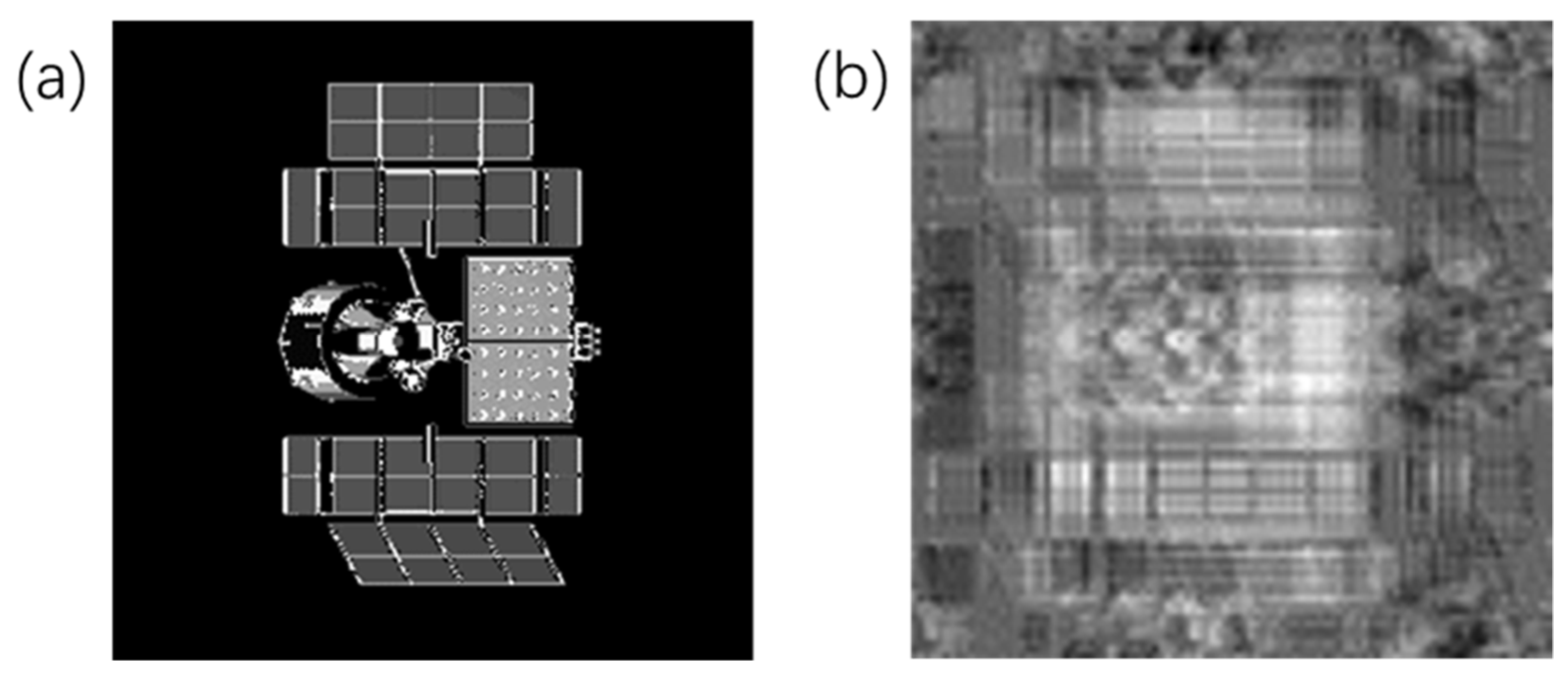
3.1.1. 3D Imaging Results of Single-Distance Target

The light collection and interference process of the photonics integrated interference imaging system was simulated and analyzed through the simulation program. The “checkerboard” imager, using a ( 2 N + 1 ) × ( 2 N + 1 ) square grid lens arrangement, was chosen, and the satellite shown in Figure 5a was chosen as the target image. The parameters of the imager and target are listed in Table 1, and the size of the target was selected as the size of FOV at this distance. The simulation process follows: the lights from the target are coupled into the optical waveguide array by the lens array and split by the demultiplexer. After passing the phase shifter, the lights are converted into a photocurrent by the balanced four quadrature detector. The corrected acquisition signal is calculated using photocurrent and reference distance, and the reconstructed image is obtained after the inverse Fourier transform.
The midpoint deviation of interference baseline is scattered in the center of four parts: (0.051 m, 0.051 m), (0.051 m, −0.050 m), (−0.050 m, 0.051 m), and (−0.050 m, −0.050 m). The reconstructed image when z c takes infinity is shown in Figure 5b, which is the result based on the signals without the correction term related to reference distance. The reconstructed image without correction has overlapping fringes due to the deviations of sub-inversion images, which leads to blur and distortion.
The reconstructed image when z c = 1500   m is shown in Figure 6a. The reconstructed image with correction using the actual distance as reference distance is clear because the deviation of each sub-inversion image is eliminated. Then, changed z c from 500 m to 2500 m to obtain the corresponding reconstructed images, and the reconstructed images when the value of z c is set to 1000 m, 1475 m, and 1550 m, respectively, are shown in Figure 6b–d. The normalized result of evaluating each reconstructed image using the evaluation function of sharpness based on the Laplace gradient function is shown by the dotted blue line in Figure 7. The normalized result of evaluating each reconstructed image using the evaluation function of sharpness based on the negative value of SSIM of the reconstructed image and the filtered image after removing the highest frequency is shown by the solid red line in Figure 7. Two evaluation functions show good unimodality. Set a search region with a certain step length near the peak, calculate the maximum value position within this region, and then set a smaller region and step near the maximum position of this region. Repeat the search process until the region length is less than 0.01 m to obtain the best reference distance. The best reference distance of evaluation functions based on gradient and SSIM are 1501.91 m and 1496.48 m, respectively. Taking 1501.91 m as the estimated distance of the target, combined with the working wavelength and the minimum baseline, the size of the reconstructed image is L c = λ z c / B min = 0.4507   m .

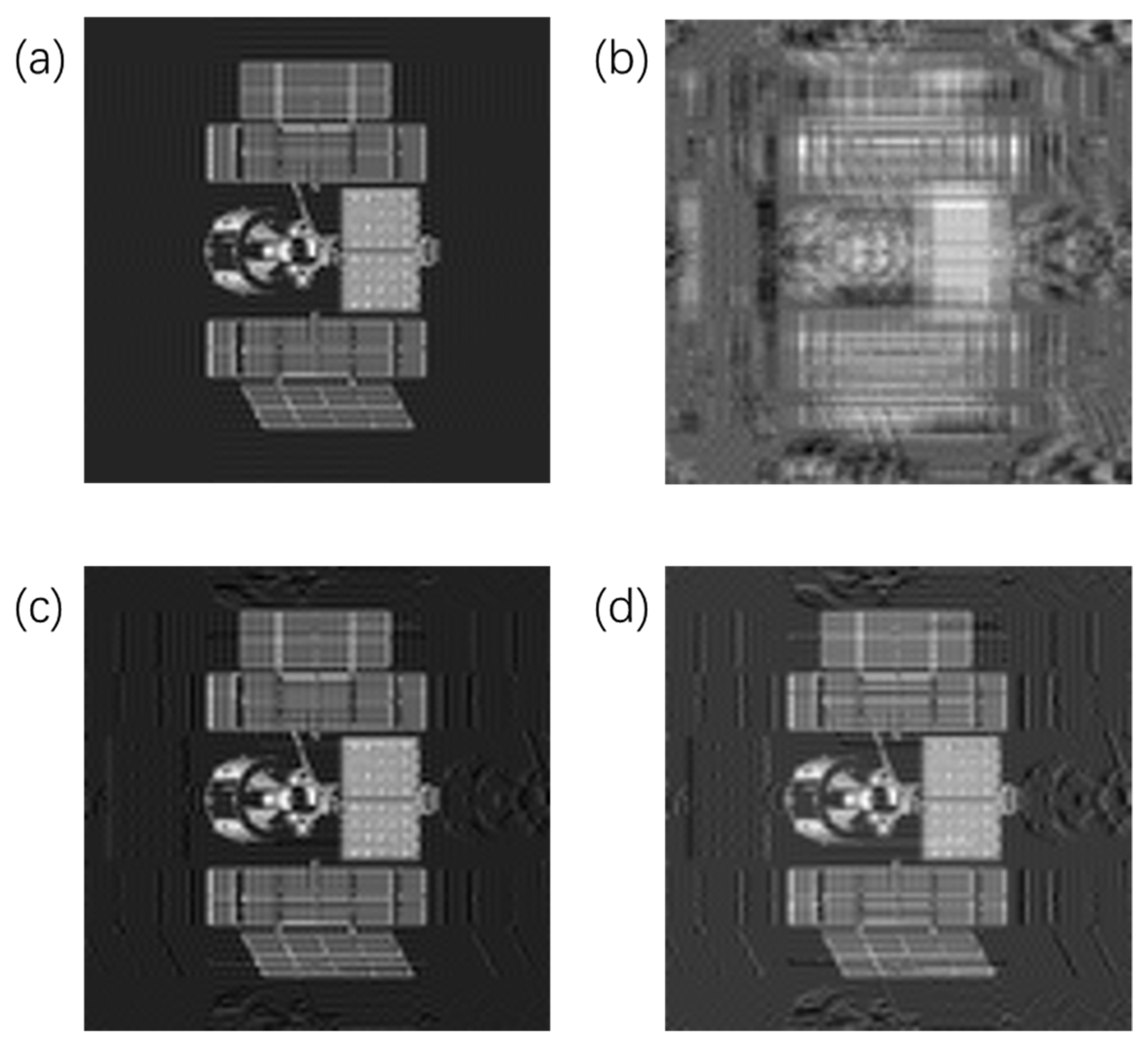
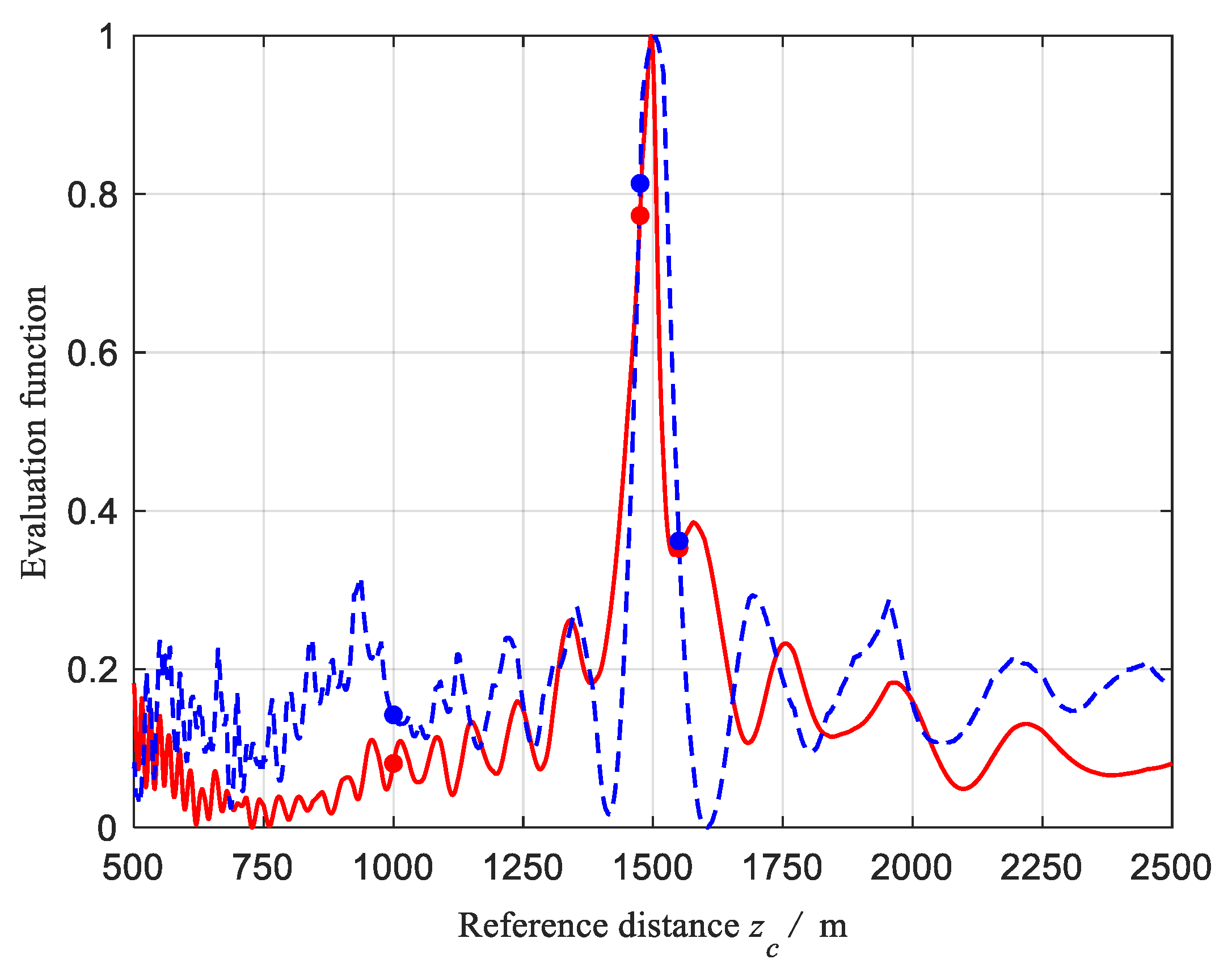
3.1.2. 3D Imaging Results of the Targets at Different Distances

The “checkerboard” lens arrangement method is still used, and the parameter N is unchanged. Select the parameters of the imager shown in Table 2, and then the midpoint deviation of interference baseline is scattered in the center of four parts: (0.0765 m, 0.0765 m), (0.0765 m, −0.0750 m), (−0.0750 m, 0.0765 m), (−0.0750 m, −0.0750 m). To verify the 3D imaging ability of this method at different working wavelengths, the working wavelength is changed to 800 nm. Set up a scene where the distances of targets occluded in the FOV are not unique. As shown in Figure 8a, the imager installed on a reconnaissance aircraft at the attitude of z 1 = 10   km is imaging a road area. The coordinate of the imager is (0 m, 0 m, 0 m) and the swath of ground is L = F O V z 1 = 24   m . An UAV flies over the road, its flying attitude is 2 km, its shape is shown in Figure 8b, its size is 1.79 m × 1.43 m, and the coordinate of its center point is (−2.19 m, −4.00 m, 8000 m). Therefore, the distance between the UAV and the imager is z 2 = 8   km . The image of the road area is shown in Figure 8c, where the red area is the projection of UAV on the ground. The “car” area used for comparison is shown in Figure 8d, where the coordinate of its center point is (3.96 m, 9.83 m, 10,000 m), and the length of the car is 2.83 m.
Following the same simulation process, the reconstructed images are obtained based on the reference distance z c varying from 6 km to 12 km. The reconstructed images of the UAV area and the “car” area are evaluated based on the Laplace gradient function, and the results are shown in Figure 9. Use interval search algorithm and take 1 m as the target precision. The best reference distances for them are 8.034 km and 9.997 km, respectively. The reconstructed images when the reference distance z c is 8.034 km and 9.997 km are shown in Figure 10a and Figure 11a, respectively. When the reference distance is set to 8.034 km, the reconstructed image of the ground part is blurry and has fringes, which is caused by the incorrect correction of the collected signals. When the reference distance is set to 9.997 km, the ground part is clear, and only the UAV are is affected. Figure 10b and Figure 11b show the reconstructed image of the “car” area. Figure 10c and Figure 11c show the reconstructed image of the UAV area. The UAV in the reconstructed image is clear, but the car is not clear when the corrected distance is close to the actual distance of UAV. In addition, the car in the reconstructed image is clear, but the UAV part is not clear when the corrected distance is close to the actual distance of the ground. Take 8.034 km as the distance of UAV. According to the relative position of the UAV in reconstructed image, its size is calculated as 1.80 m × 1.44 m, and the coordinate of its center point is calculated as (−2.20 m, −4.02 m, 8034 m). Take 9.997 km as the distance of the ground. According to the relative position of the “car” area in the reconstructed image, the coordinate of its center point is calculated as (3.96 m, 9.82 m, 9997 m), and the length of the car is calculated as 2.83 m.

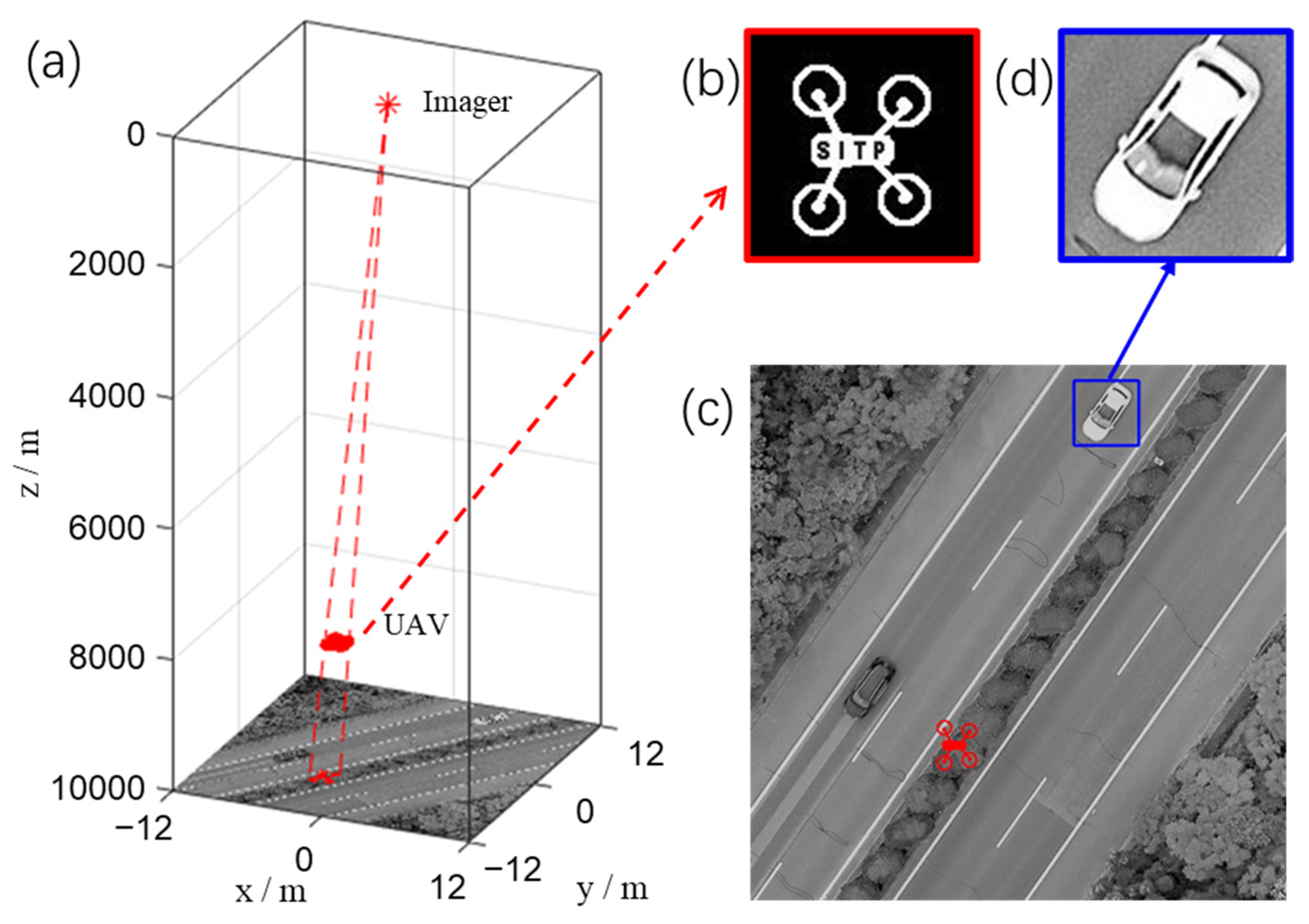
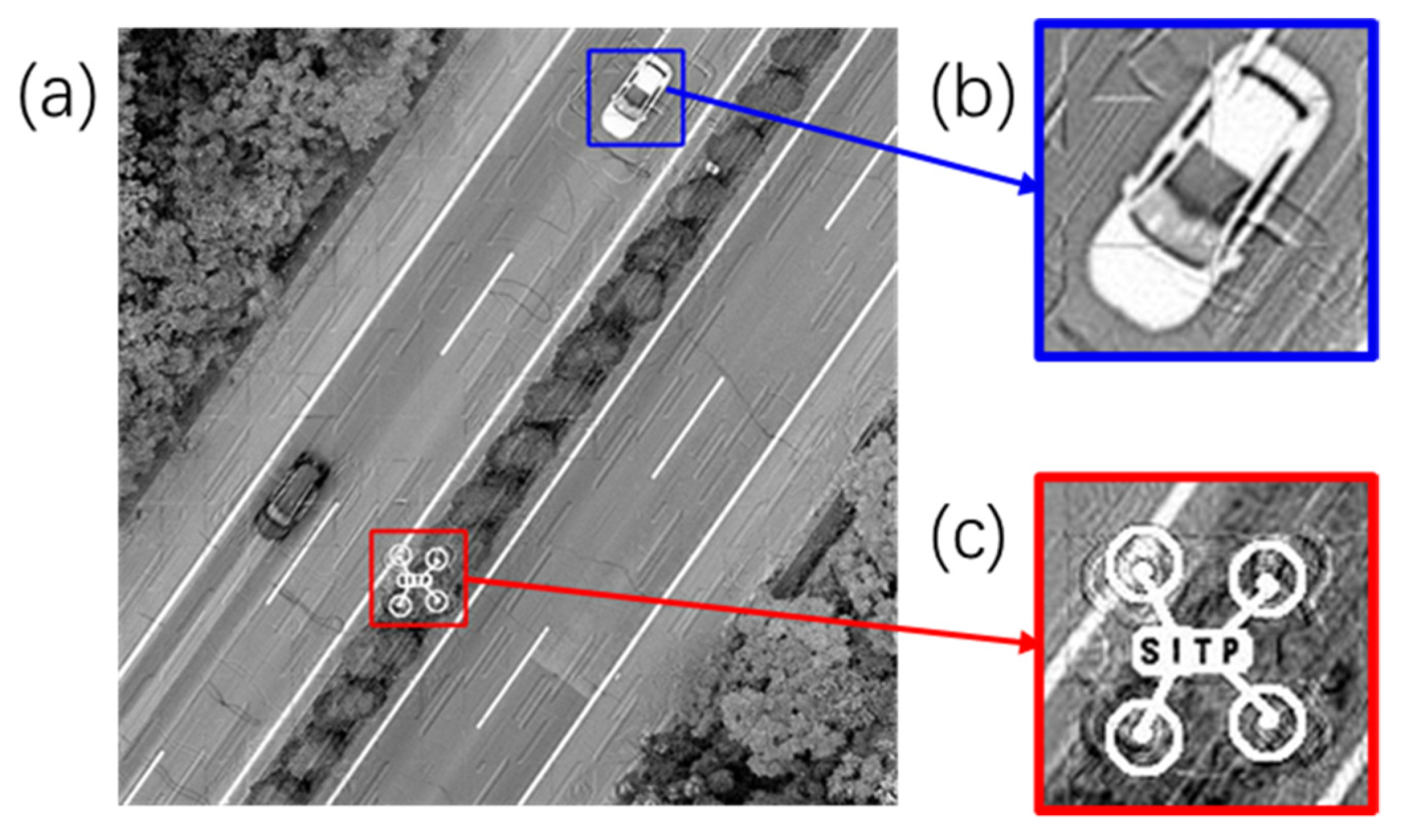
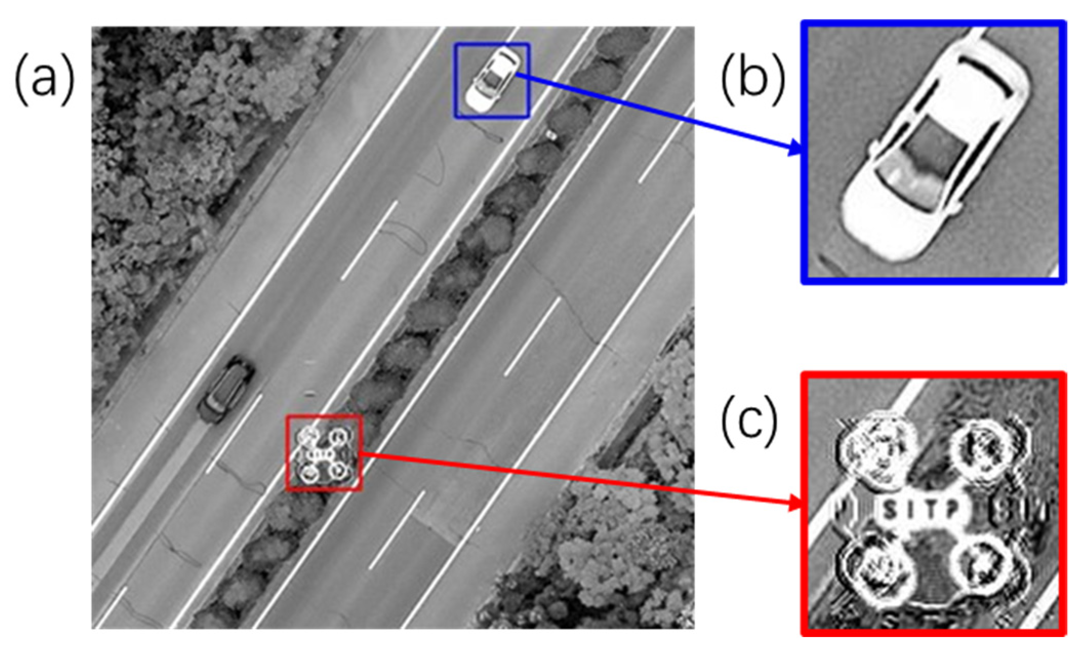
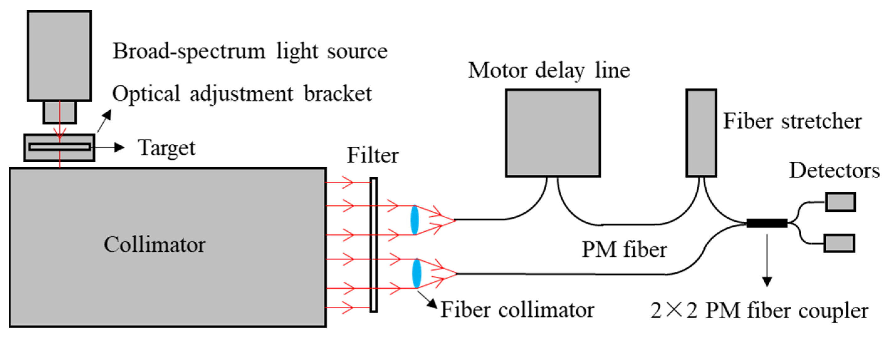
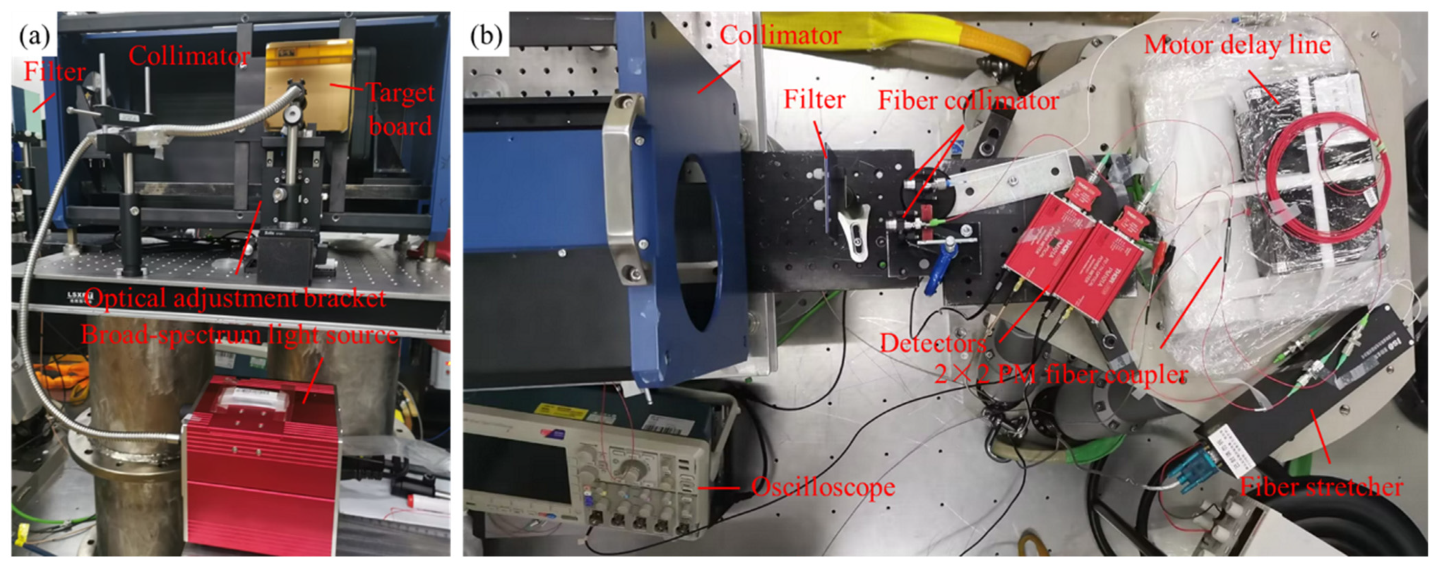
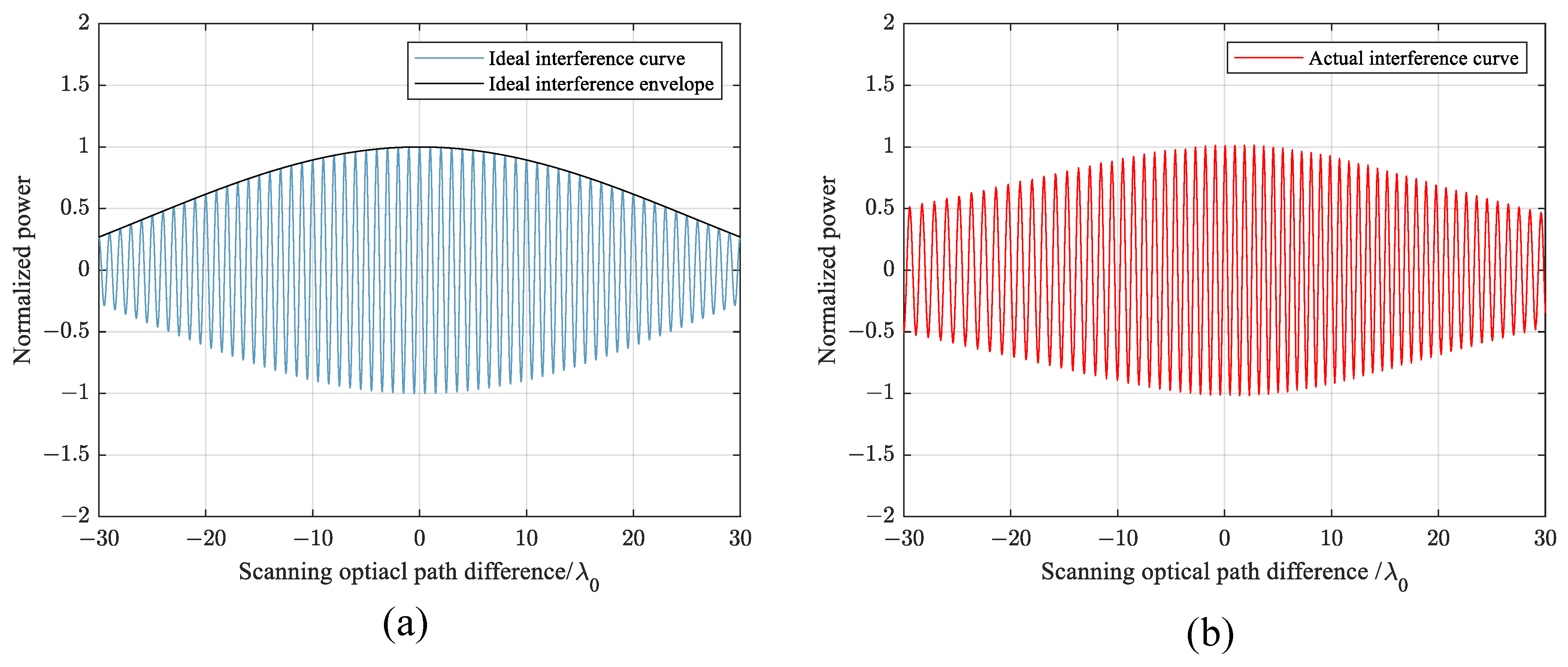
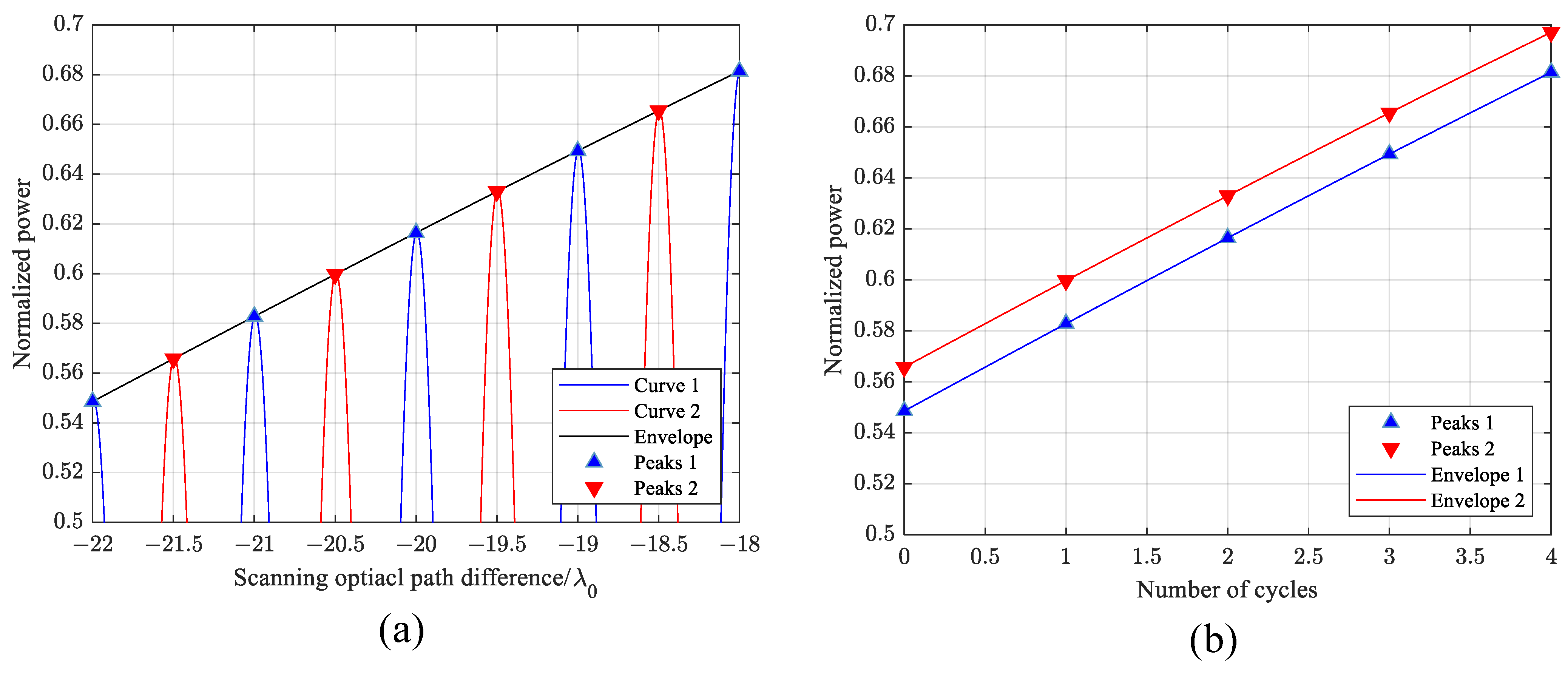
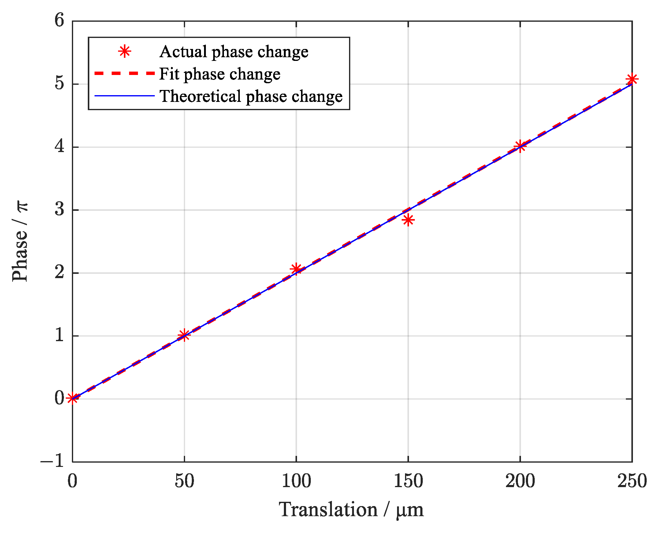
3.2. Experimental Results

In the process of optical interference imaging, the deviation of the midpoint of the interference baseline relative to the optical axis causes the phase change Δ φ = 2 π B d / λ ¯ z of the complex coherence factor, where B = ( x 2 x 1 , y 2 y 1 ) is the interference baseline, and d is the displacement of the midpoint position of the lens relative to the center of the target. The phase change of the complex coherence factor causes the spatial fringes corresponding to the interference baseline to shift in the reconstructed image, which affects the sharpness of the reconstructed image. This is the theoretical basis of the passive 3D positioning imaging method based on the photonic integrated interference imaging system. We set up an interference experiment of the broad-spectrum light and a grating composed of fixed spacing stripes as the target to verify the relationship between the relative displacement of the spatial fringe target and the center of the lens, the target distance, and the phase of the complex coherence factor, which verifies the correctness of the basic theoretical of the 3D spatial positioning imaging method proposed in this paper.
The optical fiber system is used for a verification experiment. As shown in Figure 12, the lights emitted by a broad-spectrum light source (Thorlabs OSL2IR) pass through the target. Then, the lights are collimated by the collimator with a focal length of 2.27 m and filtered by the filter with a filtering range of 1550 nm ± 20 nm. Two fiber collimators with a distance of d collected the lights. One ray of lights passes through the motor delay line and the fiber stretcher, and then interferes with the other ray of lights through 2 × 2 optical fiber coupler. The fiber stretcher with large range and step length is used to initially find the equal optical path position, and the motor delay line with small range and step length is used to scan the interference curve near the equal optical path position. Finally, the detectors are used to collect two interference signals with opposite phase after interference. The image of the experimental equipment is shown in Figure 13.
A grating pattern with a side length of 2 mm and the light and dark stripe width of 50 μm respectively is used as the target. The fiber collimators are set with a distance of B = 3.5   cm and obtain a distance of z = 2.27   m from the target. Translate the target in the direction parallel to the interference baseline by Δ d to change the distance between the midpoint of fiber collimators and the optical axis. The phase change caused by the translation is:
Δ φ = 2 π λ z Δ d B .
This means that the phase will change one period when the target is moved by λ z / B = 100   μ m .
The target is translated from 0 to 250 μm through an optical adjustable mount, and the interference curve of each position is measured four times by adjusting the motor delay line. The interference curve of ideal light distribution is:
I = I b g Δ ν { 1 + η sin c ( Δ ν τ ) cos [ arg ( μ ) + 2 π ν 0 τ ] } .
where I b g = I 1 + I 2 is the light intensity of the two rays of lights, η = 2 I 1 I 2 | μ | I 1 + I 2 is fringe visibility, and τ is the optical path difference between two rays of lights. As shown in Figure 14a, the ideal interference envelope is a sinc curve after removing the direct current component.
In the actual experiment, the non-ideal light intensity distribution, the dispersion effect caused by long optical fiber, the vibration of the optical fiber, and the noise change the shape of the interference curve, as shown in Figure 14b. The non-ideal light source and dispersion effect reduce the extreme value of the envelope and increase the distance of the first zero point. The vibration of the optical fiber introduces additional random phase difference changes, resulting in the scanning time no longer linearly corresponding to the actual optical path difference changes. The phase difference between each peak in the curve is a period, so this paper calculates the phase difference between different interference curves using the peaks of the interference curve after low pass filtering and normalization.
As shown in Figure 15, the peaks of two interference curves with different phases of complex coherence factors fall on the same interference envelope. Reassign the peaks of the two curves with the number of cycles as the abscissa, then the interference envelope formed by the two groups of peaks has translation. The translation amount is the phase difference of the complex coherence factor of two curves. The phase change of each position is analyzed based on the initial position, and the relationship between the unwrapped phase and the translation is shown in Figure 16, which matches the theoretical variation.

4. Discussion

The simulation results of the single range target show that the sharpness of the reconstructed image can be changed by adjusting the reference distance. By using the image sharpness evaluation algorithm to evaluate the target reconstruction images at different reference distances, the evaluation function curve shows a good unimodality. The estimated distance and size of the target obtained by searching the peak position of the evaluation function curve through the interval search algorithm are very close to the actual distance and size. The evaluation function based on negative SSIM has smaller oscillations when the corrected distance is far from the actual distance, and has a smaller full width at half maximum (FWHM) near the actual distance, but it is only suitable for evaluating the overall image because it requires high-frequency image information. The performance of the evaluation function based on the gradient can be used to analyze local patterns. The positioning errors of the two evaluation functions are 1.91 m and 3.52 m, respectively, which can be expressed as 0.127% at 1500 m and 0.234% at 1500 m.
The simulation results of targets with different distances show that the sharpness of different target images in the reconstructed image can be changed by adjusting the reference distance. The evaluation function of each target image shows a good unimodality near its actual distance. The distance, size, and clear image of the target at different distances can be obtained by the interval search algorithm. The positioning error of the UAV target is 34 m, which can be expressed as 0.425% at 8000 m, and the positioning error of the ground car target is 3 m, which can be expressed as 0.030% at 10,000 m. Because the positioning work depends on the sharpness evaluation of the target reconstructed image, the feature texture of the target affects the sensitivity of the evaluation function. Choosing the evaluation function sensitive to gradient change and high frequency change, as well as the target with complex texture, will improve the positioning accuracy to a certain extent.
The accuracy of the passive 3D imaging method proposed in this paper cannot match an active imaging method, such as lidar. However, it is close to 0.833% at 60 m [6] of monocular estimation method, 0.140%, 0.095%, and 0.049% at 200 m [7] and 2.157% at 100 cm [8] of stereo vision method, 0.034%, 0.028%, and 0.047% at 200 m [10] and 0.568~0.787% at 38.5~53.3 m [11] of the oblique photography method. Compared with the stereo vision method and oblique photography method for 3D reconstruction of point cloud, our method is to locate and image the discrete distance target, respectively. Limited by the interference principle, our method has a minimum working distance. Using the imager parameters shown in Table 1, and assuming a bandwidth of 20 nm, the theoretical minimum working distance of the system is calculated to be 283.33 m according to Formula (14). Thanks to the small size, weight, and power consumption of the photonic integrated interference imaging system due to its high integration, our method can also choose UAV, airship, and satellite as the carrying platform.
The research on the photonic integrated interferometric imaging system is still in the primary stage. Only a few studies have reported the PIC chip with interferometer elements [14,29,30,31], and no prototype has been fabricated. The imaging of complex targets is still very difficult. Therefore, we selected the simplest fringe target for basic principle verification, which was based on the relationship between the relative displacement of the spatial fringe and the midpoint of the interference baseline, the target distance, and the phase of the complex coherence factor. We measured the wide-spectrum optical interference signal curves of different fringe target translations. By analyzing the phase difference of the complex coherence factor corresponding to each interference curve, we calculated the phase of the complex coherence factor measured by the interference baseline with a length of 3.5 cm change π for 50 μm movement of the fringe target at an imaging distance of 2.27 m. It shows that the variation of spatial translation, target distance, and complex coherence factor phase is consistent with the theory: Δ φ = 2 π B d / λ ¯ z , which indirectly verifies the correctness of the basic theory of the proposed method. However, due to the limitations of the experimental conditions, we do not have the conditions to directly obtain the phase of the complex coherence factor measured by the interference baseline, so that the reconstructed image of the target cannot be obtained directly, which is a key problem to be solved.

5. Conclusions

3D positioning imaging methods are an important part of planetary, lunar, and deep space exploration. Various 3D imaging methods have been proposed, and all traditional passive 3D imaging methods are based on diffraction imaging technology. The photonics integrated interference imaging system based on interference imaging collects the complex coherence factor of object light, which is closely related to object distance, and gives passive 3D imaging method new enlightenment. This paper discusses the conditions for reconstructing clear images from the complex coherence factor collected by the photonics integrated interference imaging system at the limited working distance and shows that adjusting the reference distance can significantly affect the sharpness of the reconstructed image when using an imager with a complex lens array. The midpoints of the interference baselines formed by these lenses are not completely overlapped. The distance between the optical axis and the two lenses of the interference baseline are not equal. Based on this, a single exposure passive 3D imaging method is proposed in this paper. The positioning accuracy of this method is related to the value and dispersion of the “image deviation”. Increasing the parameters of the lens array, increasing the distribution distance of the midpoints of the interference array, reducing the target distance, and working wavelength can improve the positioning accuracy.
This article proves that the photonics integrated interference imaging system can acquire 3D information of the target, which may provide a new method and idea for the design of the imagers. This paper provides a new passive 3D positioning and imaging scheme with higher integration, that is faster and more convenient for the field of planetary, lunar, and deep space exploration.

Author Contributions

Conceptualization, B.G. and Q.Y.; methodology, B.G. and Q.Y.; software, B.G.; validation, B.G. and J.C.; formal analysis, B.G.; investigation, B.G.; resources, Q.Y.; data curation, B.G. and Q.Y.; writing—original draft preparation, B.G.; writing—review and editing, Q.Y. and S.S.; visualization, B.G.; supervision, Q.Y.; project administration, Q.Y. and S.S.; funding acquisition, Q.Y. All authors have read and agreed to the published version of the manuscript.

Funding

This study was funded by National Natural Science Foundation of China (No. 62105350) and the Youth Innovation Promotion Association of the Chinese Academy of Sciences (No. Y201951).

Data Availability Statement

Not applicable.

Acknowledgments

We express our sincere thanks to Chuang Zhang, He Yan and other fellow students at Shanghai Institute of Technical Physics of Chinese Academy of Sciences, who reviewed the original paper and provided valuable comments.

Conflicts of Interest

The authors declare no conflict of interest.

References

  1. Geng, J. Structured-Light 3D Surface Imaging: A Tutorial. Adv. Opt. Photonics 2011, 3, 128. [Google Scholar] [CrossRef]
  2. Hu, Y.; Chen, Q.; Feng, S.; Zuo, C. Microscopic Fringe Projection Profilometry: A Review. Opt. Lasers Eng. 2020, 135, 106192. [Google Scholar] [CrossRef]
  3. Zhang, M.; Chen, Q.; Tao, T.; Feng, S.; Hu, Y.; Li, H.; Zuo, C. Robust and Efficient Multi-Frequency Temporal Phase Unwrapping: Optimal Fringe Frequency and Pattern Sequence Selection. Opt. Express 2017, 25, 20381. [Google Scholar] [CrossRef]
  4. Li, Z.-P.; Huang, X.; Jiang, P.-Y.; Hong, Y.; Yu, C.; Cao, Y.; Zhang, J.; Xu, F.; Pan, J.-W. Super-Resolution Single-Photon Imaging at 8.2 Kilometers. Opt. Express 2020, 28, 4076. [Google Scholar] [CrossRef] [PubMed]
  5. Li, Z.-P.; Ye, J.-T.; Huang, X.; Jiang, P.-Y.; Cao, Y.; Hong, Y.; Yu, C.; Zhang, J.; Zhang, Q.; Peng, C.-Z.; et al. Single-Photon Imaging over 200 Km. Optica 2021, 8, 344. [Google Scholar] [CrossRef]
  6. Zhe, T.; Huang, L.; Wu, Q.; Zhang, J.; Pei, C.; Li, L. Inter-Vehicle Distance Estimation Method Based on Monocular Vision Using 3D Detection. IEEE Trans. Veh. Technol. 2020, 69, 4907–4919. [Google Scholar] [CrossRef]
  7. Wang, Y.; Wang, X. On-Line Three-Dimensional Coordinate Measurement of Dynamic Binocular Stereo Vision Based on Rotating Camera in Large FOV. Opt. Express 2021, 29, 4986. [Google Scholar] [CrossRef]
  8. Adil, E.; Mikou, M.; Mouhsen, A. A Novel Algorithm for Distance Measurement Using Stereo Camera. CAAI Trans. Intell. Technol. 2022, 7, 177–186. [Google Scholar] [CrossRef]
  9. Xingyu, Y.; Yanduo, Z.; Yuechao, Z.; Yuan, Z.; Alang, L.; Xiao, C.; Chunhui, P.; Jianchao, Z.; Yakun, Z.; Xianglan, D. Research on Multi Baseline Large Depth 3D Imaging. In Proceedings of the 2022 International Conference on Computer Engineering and Artificial Intelligence (ICCEAI), Shijiazhuang, China, 22–24 July 2022; pp. 339–343. [Google Scholar]
  10. Xi, W.; Zuo, X.; Xiao, B.; Zhu, J.; Zhou, D. The Construction and Precision Analysis of the Three—Dimensional Oblique Photogrammetry Model. In Proceedings of the 2021 28th International Conference on Geoinformatics, Nanchang, China, 3 November 2021; pp. 1–5. [Google Scholar]
  11. Qiu, Y.; Jiao, Y.; Luo, J.; Tan, Z.; Huang, L.; Zhao, J.; Xiao, Q.; Duan, H. A Rapid Water Region Reconstruction Scheme in 3D Watershed Scene Generated by UAV Oblique Photography. Remote Sens. 2023, 15, 1211. [Google Scholar] [CrossRef]
  12. Kendrick, R.L.; Duncan, A.; Ogden, C.; Wilm, J.; Stubbs, D.M.; Thurman, S.T.; Su, T.; Scott, R.P.; Yoo, S. Flat-Panel Space-Based Space Surveillance Sensor. In Proceedings of the Advanced Maui Optical and Space Surveillance Technologies (AMOS) Conference, Maui, HI, USA, 10–13 September 2013. [Google Scholar]
  13. Thurman, S.T.; Kendrick, R.L.; Duncan, A.; Wuchenich, D.; Ogden, C. System Design for a SPIDER Imager. In Proceedings of the Frontiers in Optics, San Jose, CA, USA, 18–22 October 2015; p. FM3E.3. [Google Scholar]
  14. Su, T.; Liu, G.; Badham, K.E.; Thurman, S.T.; Kendrick, R.L.; Duncan, A.; Wuchenich, D.; Ogden, C.; Chriqui, G.; Feng, S.; et al. Interferometric Imaging Using Si3N4 Photonic Integrated Circuits for a SPIDER Imager. Opt. Express 2018, 26, 12801. [Google Scholar] [CrossRef]
  15. Kendrick, R.L.; Duncan, A.; Ogden, C.; Wilm, J.; Thurman, S.T. Segmented Planar Imaging Detector for EO Reconnaissance. In Proceedings of the Imaging and Applied Optics, Arlington, VI, USA, 23–27 June 2013; p. CM4C.1. [Google Scholar]
  16. Duncan, A.; Kendrick, R.; Thurman, S.; Wuchenich, D.; Scott, R.P.; Yoo, S.; Su, T.; Yu, R.; Ogden, C.; Proiett, R. SPIDER: Next Generation Chip Scale Imaging Sensor. In Proceedings of the Advanced Maui Optical and Space Surveillance Technologies Conference, Maui, HI, USA, 15–18 September 2015; p. 27. [Google Scholar]
  17. Chu, Q.; Shen, Y.; Yuan, M.; Gong, M. Numerical Simulation and Optimal Design of Segmented Planar Imaging Detector for Electro-Optical Reconnaissance. Opt. Commun. 2017, 405, 288–296. [Google Scholar] [CrossRef]
  18. Debary, H.; Mugnier, L.M.; Michau, V. Aperture Configuration Optimization for Extended Scene Observation by an Interferometric Telescope. Opt. Lett. 2022, 47, 4056. [Google Scholar] [CrossRef]
  19. Gao, W.P.; Wang, X.R.; Ma, L.; Yuan, Y.; Guo, D.F. Quantitative Analysis of Segmented Planar Imaging Quality Based on Hierarchical Multistage Sampling Lens Array. Opt. Express 2019, 27, 7955. [Google Scholar] [CrossRef] [PubMed]
  20. Gao, W.; Yuan, Y.; Wang, X.; Ma, L.; Zhao, Z.; Yuan, H. Quantitative Analysis and Optimization Design of the Segmented Planar Integrated Optical Imaging System Based on an Inhomogeneous Multistage Sampling Lens Array. Opt. Express 2021, 29, 11869. [Google Scholar] [CrossRef]
  21. Lv, G.; Chen, Y.; Feng, H.; Xu, Z.; Li, Q. System Design for an Improved SPIDER Imager. In Proceedings of the 6th China High Resolution Earth Observation Conference (CHREOC 2019); Wang, L., Wu, Y., Gong, J., Eds.; Lecture Notes in Electrical Engineering; Springer: Singapore, 2020; Volume 657, pp. 241–259. ISBN 9789811539466. [Google Scholar]
  22. Ming, Z.; Liu, Y.; Li, S.; Zhou, M.; Du, H.; Zhang, X.; Zuo, Y.; Qiu, J.; Wu, J.; Gao, L.; et al. Optimal Design of Segmented Planar Imaging System Based on Rotation and CLEAN Algorithm. Photonics 2023, 10, 46. [Google Scholar] [CrossRef]
  23. Yong, J.; Feng, Z.; Wu, Z.; Ye, S.; Li, M.; Wu, J.; Cao, C. Photonic Integrated Interferometric Imaging Based on Main and Auxiliary Nested Microlens Arrays. Opt. Express 2022, 30, 29472. [Google Scholar] [CrossRef]
  24. Ding, C.; Zhang, X.; Liu, X.; Meng, H.; Xu, M. Structure Design and Image Reconstruction of Hexagonal-Array Photonics Integrated Interference Imaging System. IEEE Access 2020, 8, 139396–139403. [Google Scholar] [CrossRef]
  25. Yu, Q.; Ge, B.; Li, Y.; Yue, Y.; Chen, F.; Sun, S. System Design for a “Checkerboard” Imager. Appl. Opt. 2018, 57, 10218. [Google Scholar] [CrossRef]
  26. Chen, T.; Zeng, X.; Zhang, Z.; Zhang, F.; Bai, Y.; Zhang, X. REM: A Simplified Revised Entropy Image Reconstruction for Photonics Integrated Interference Imaging System. Opt. Commun. 2021, 501, 127341. [Google Scholar] [CrossRef]
  27. Ding, C.; Zhang, X.; Liu, X.; Meng, H.; Xu, M. High-Resolution Reconstruction Method of Segmented Planar Imaging Based on Compressed Sensing. In Proceedings of the Advanced Optical Imaging Technologies II, Hangzhou, China, 21–23 October 2019; Carney, P.S., Yuan, X.-C., Shi, K., Somekh, M.G., Eds.; SPIE: Hangzhou, China, 2019; p. 4. [Google Scholar]
  28. Zhang, Z.; Li, H.; Lv, G.; Zhou, H.; Feng, H.; Xu, Z.; Li, Q.; Jiang, T.; Chen, Y. Deep Learning-Based Image Reconstruction for Photonic Integrated Interferometric Imaging. Opt. Express 2022, 30, 41359. [Google Scholar] [CrossRef]
  29. Chen, H.; On, M.B.; Lee, Y.J.; Zhang, L.; Proietti, R.; Ben Yoo, S.J. Photonic Interferometric Imager with Monolithic Silicon CMOS Photonic Integrated Circuits. In Proceedings of the Optical Fiber Communication Conference (OFC), San Diego, CA, USA, 6–10 March 2022; Optica Publishing Group: San Diego, CA, USA, 2022; p. Tu2I.2. [Google Scholar]
  30. Zhang, Y.; Wang, K.; An, Q.; Hao, Y.; Meng, H.; Liu, X. High-Accuracy Online Calibration Scheme for Large-Scale Integrated Photonic Interferometric Measurements. IEEE Photonics J. 2022, 14, 1–5. [Google Scholar] [CrossRef]
  31. Liu, S.; Chen, Z.; Ye, Z.; Qi, Y.; Zhao, H.; Qu, Z.; Lu, J.; Wang, Y.; Han, C. Optical Direction-Finding Based on Silicon Photonic Integrated Circuits. J. Light. Technol. 2023, 41, 2650–2656. [Google Scholar] [CrossRef]
  32. Yu, Q.; Wu, D.; Chen, F.; Sun, S. Design of a Wide-Field Target Detection and Tracking System Using the Segmented Planar Imaging Detector for Electro-Optical Reconnaissance. Chin. Opt. Lett. 2018, 16, 071101. [Google Scholar] [CrossRef]
  33. Chen, J.; Ge, B.; Yu, Q. Influence of Measurement Errors of the Complex Coherence Factor on Reconstructed Image Quality of Integrated Optical Interferometric Imagers. Opt. Eng. 2022, 61, 105108. [Google Scholar] [CrossRef]
  34. Hui, L.; Chengyu, F. An Improved Focusing Algorithm Based on Image Definition Evaluation. In Proceedings of the 2011 2nd International Conference on Artificial Intelligence, Management Science and Electronic Commerce (AIMSEC), Dengfeng, China, 8–10 August 2011; pp. 3743–3746. [Google Scholar]
  35. Wang, Z.; Bovik, A.C.; Sheikh, H.R.; Simoncelli, E.P. Image Quality Assessment: From Error Visibility to Structural Similarity. IEEE Trans. Image Process. 2004, 13, 600–612. [Google Scholar] [CrossRef] [PubMed]
Figure 1. The structure of the “checkerboard” imager.
Remotesensing 15 02333 g001
Figure 2. 2D schematic diagram of the imager.
Remotesensing 15 02333 g002
Figure 3. The principle of obtaining a reconstructed image. (a) The object space can be decomposed into a series of sub-original images. (b) The sub-inversion images without deviation constitute a clear reconstructed image. (c) The sub-inversion images with same deviation constitute a clear but biased reconstructed image. (d) The sub-inversion images with different deviation constitute a blurred reconstructed image.
Remotesensing 15 02333 g003
Figure 4. Flow chart of the method described in this paper.
Remotesensing 15 02333 g004
Figure 5. (a) Target image of computer simulation. (b) The reconstructed image without correction (The reference distance takes infinity).
Remotesensing 15 02333 g005
Figure 6. The reconstructed image when the reference distance is (a) 1500 m, (b) 1000 m, (c) 1475 m, and (d) 1550 m respectively.
Remotesensing 15 02333 g006
Figure 7. The relationship between the sharpness of the reconstructed image and the value of the reference distance, which is evaluated by the Laplacian gradient function (dotted blue line) and the negative SSIM (solid red line), respectively. The abscissa sampling step in the main drawing is 1 m, and the abscissa sampling step in the sub-drawing is 0.05 m.
Remotesensing 15 02333 g007
Figure 8. The scene of 3D imaging simulation. (a) The spatial position of the imager, UAV, and ground. (b) The shape of UAV. (c) The image of ground with a red area which is the projection of the UAV. (d) The image of the “car” area.
Remotesensing 15 02333 g008
Figure 9. The relationship between the sharpness of the reconstructed image and the value of the reference distance, which is evaluated by the Laplacian gradient function. The abscissa sampling step is 10 m.
Remotesensing 15 02333 g009
Figure 10. The simulation results of (a) the reconstructed image, (b) the “car” area and (c) the UAV area when the reference distance is 8.034 km.
Remotesensing 15 02333 g010
Figure 11. The simulation results of (a) the reconstructed image, (b) the “car” area and (c) the UAV area when the reference distance is 9.997 km.
Remotesensing 15 02333 g011
Figure 12. Schematic diagram of interference experiment device.
Remotesensing 15 02333 g012
Figure 13. The image of the experimental equipment. (a) The front optical path. (b) The backend optical path.
Remotesensing 15 02333 g013
Figure 14. (a) Ideal interference curve and envelope. (b) The interference curve obtained in actual experiment.
Remotesensing 15 02333 g014
Figure 15. Interference curve and envelope with different phases of complex coherence factor, where the phase of the complex coherence factor of the curve 1, peaks 1, envelope 1 is 0, and the phase of the complex coherence factor of the curve 2, peaks 2, envelope 2 is π. (a) The data take the value of scanning optical path difference divided by the wavelength as the abscissa. (b) The data take the number of cycles as the abscissa.
Remotesensing 15 02333 g015
Figure 16. The relationship between the unwrapped phase change and the translation.
Remotesensing 15 02333 g016
Table 1. The parameters of the imager and target for the simulation of single-distance target.
ParameterValue
Array parameter N 50
Size of the lens array101 × 101
Minimum baseline B min 0.002 m
Diameter of the d 0.002 m
Diameter of system D 0.283 m
Size of the waveguide array after each lens1 × 1
Working wavelength λ 600 nm
FOV0.0172°
Distance of target z 1500 m
Width of FOV of single waveguide L 0.450 m
Table 2. The parameters of the imager and target for the simulation of the targets at different distances.
ParameterValue
Array parameter N 50
Size of the lens array101 × 101
Minimum baseline B min 0.003 m
Diameter of the d 0.002 m
Diameter of system D 0.424 m
Size of the waveguide array after each lens9 × 9
Working wavelength λ 800 nm
FOV0.1375°
The distance of the ground and the car z 1 10 km
The length of the car2.83 m
The distance of the UAV z 2 8 km
The size of the UAV1.79 m × 1.43 m
Disclaimer/Publisher’s Note: The statements, opinions and data contained in all publications are solely those of the individual author(s) and contributor(s) and not of MDPI and/or the editor(s). MDPI and/or the editor(s) disclaim responsibility for any injury to people or property resulting from any ideas, methods, instructions or products referred to in the content.

