Thaw-Season InSAR Surface Displacements and Frost Susceptibility Mapping to Support Community-Scale Planning in Ilulissat, West Greenland

Abstract

In permafrost regions, ground surface deformations induced by freezing and thawing threaten the integrity of the built environment. Mapping the frost susceptibility of the ground at a high spatial resolution is of practical importance for the construction and planning sectors. We processed Sentinel-1 Interferometric Synthetic Aperture Radar (InSAR) data from thawing seasons 2015 to 2019, acquired over the area of Ilulissat, West Greenland. We used a least-squares inversion scheme to retrieve the average seasonal displacement (S) and long-term deformation rate (R). We secondly investigated two different methods to extrapolate active layer thickness (ALT) measurements, based on their statistical relationship with remotely sensed surface characteristics. A generalized linear model (GLM) was first implemented, but the model was not able to fit the data and represent the ALT spatial variability over the entire study domain. ALT were alternatively averaged per vegetation class, using a land cover map derived by supervised classification of Sentinel-2 images. We finally estimated the active layer ice content and used it as a proxy to map the frost susceptibility of the ground at the community scale. Fine-grained sedimentary basins in Ilulissat were typically frost susceptible and subject to average seasonal downward displacements of 3 to 8 $\mathrm{cm}$. Areas following a subsiding trend of up to 2.6 $\mathrm{cm}/\mathrm{yr}$ were likely affected by permafrost degradation and melting of ground ice below the permafrost table. Our approach enabled us to identify frost-susceptible areas subject to severe seasonal deformations, to long-term subsidence induced by degrading permafrost, or to both. Used in combination with traditional site investigations, InSAR maps provide valuable information for risk management and community planning in the Arctic.

1. Introduction

Building on frozen ground entails many geotechnical implications related to the properties and thermal regime of the ground [1]. Ground heave and subsidence induced by seasonal freezing and thawing of the active layer (AL) generate stresses on infrastructures that can lead to damage and failures. In permafrost terrain, climate change, in conjunction with anthropogenic disturbances, has furthermore caused an increase in ground temperature and deepening of the active layer [2,3]. As a result, loss of bearing capacity [4,5,6,7], seasonal and long-term ground subsidence, e.g., [8,9,10], have been observed across the Arctic due to melting of the ground ice and soil consolidation. These changes severely threaten the integrity of the built environment and increasingly expose Arctic communities to hazards [11,12]. It is therefore paramount to adapt construction designs and mitigation solutions to frost conditions and thermal regime changes. In this context, the monitoring of ground surface deformations can serve as a powerful tool to manage permafrost-induced risks and to support community planning.

The occurrence and magnitude of surface deformations is primarily controlled by the frost susceptibility of the ground, defined as the proneness of the ground (soil or rock) to form segregated ice (causing frost heave) under the required conditions of moisture supply and temperature [13]. Frost susceptibility, soil particle size and ground ice content thereby strongly interrelate. Yet, assessing the spatial distribution of frost-susceptible soils remains very complex. Determining ground properties and quantifying ground ice content typically require drilling and retrieving soil material for analyses. Such geotechnical investigations are costly, labor intensive, and logistically challenging in Arctic environments. Furthermore, sample extraction only provides punctual information in space and time and hence is limited in portraying the complex spatial heterogeneity and temporal evolution of subsurface properties under climate change [14].

Remote sensing techniques provide continuous spatial information in areas where the acquisition of in situ data remains challenging. In this context, the potential of Interferometric Synthetic Aperture Radar (InSAR) has been extensively explored in the past years to monitor surface deformations in permafrost environments with a high spatial resolution [15]. Prior research has primarily been dedicated to develop InSAR techniques for the comprehension of freezing/thawing dynamics of the AL and identification of driving factors explaining the magnitude of ground movements [9,16,17,18,19,20,21,22,23]. It is worth mentioning the approach proposed by Liu et al. [16] and Schaefer et al. [24] who developed an active layer thickness (ALT) retrieval algorithm, based on the relationship between the thaw depth and InSAR-derived surface displacement. By using synthetic aperture radar (SAR) scenes covering several thawing seasons, the authors were able to identify a seasonal and a long-term component in the remotely sensed displacement signal. Seasonal subsidence was attributed to thaw settlement, caused by phase and volume changes occurring in the AL upon thawing, while long-term subsidence was explained by permafrost degradation and melting of the ice at the top of permafrost. Under the assumption that the seasonal subsidence can be related to the volume of melted ice in the AL, they finally estimated ALT from the InSAR measurements by modeling the vertical distribution of the pore water within the AL.

Despite these advances, little work has been undertaken to map subsurface properties—such as the frost susceptibility or ground ice content—that are of practical interest to actors from the construction and planning sectors. In their paper, Zwieback and Meyer [14] notably explained the difficulty of deriving permafrost ground ice from remote sensing data and stressed the limitations of traditional mapping techniques, currently relying on expert knowledge and surface indicators of excess ice [25]. In an attempt to overcome these challenges, the authors assessed the suitability of late-season subsidence derived from InSAR, to identify the presence of ice-rich materials at the top of permafrost [14]. They hypothesized that ice melting under the permafrost table occurs when the thaw front penetrates frozen material toward the end of a warm summer season. Consequently, the thawing of ice-rich top-of-permafrost would induce a peculiar acceleration of the InSAR late-season subsidence. Their methodology proved to be most successful in the case of exceptionally warm and wet summers, but the separability of late-season subsidence signals from ice-rich versus ice-poor areas was reduced under cooler conditions. Those findings agree with Bartsch et al. [20], which documented higher-than-average subsidence in an exceptionally warm summer in regions known for the presence of tabular ground ice at the base of the active layer. Differences between landcover types (representing differences in soil properties) were, however, found.

Overall, InSAR techniques have rarely been used in an engineering context to prevent the occurrence of infrastructure failures [10,26] and to help governmental and planning entities make informed decisions. Arctic communities could benefit from multi-disciplinary approaches combining remote sensing and geotechnical data, at a time when adaptation strategies are urgently needed in response to climate change [27,28].

Many Greenland settlements are facing the challenges previously mentioned. Due to limited resources and logistical constraints, detailed site investigations are rarely performed prior to construction projects. Available geotechnical information is hence scarce or not easily accessible, and construction designs are not sufficiently adapted to local sub-surface conditions [27]. As a result, stability issues frequently affect existing infrastructure and particularly roads crossing ice-rich sedimentary basins. Like in other regions of the Arctic, stakeholders have expressed their interest in reliable decision support tools to guide urban planning on sensitive permafrost terrain and to identify suitable mitigation solutions.

In order to address Greenlandic stakeholders’ needs, we revisited the methodology of Liu et al. [16] and used InSAR data to map surface deformation trends in Ilulissat, West Greenland. Previous tests for Illulisat indicated applicability for seasonal as well as for long-term change monitoring applications [6,15]. We combine the InSAR results with local information to prepare a frost susceptibility index (FSI) map of the region.

2. Study Area

Our study area is the settlement of Ilulissat (Figure 1a), which is centrally located on the west coast of Greenland (69.2198${}^{\circ }$ N, 51.0986${}^{\circ }$ W) and is the seat of the Avannaata municipality. Ilulissat is the third largest town in Greenland and is an attractive tourist destination due to its proximity to the UNESCO World Heritage Site Ilulissat Icefjord. For these reasons and due to the current construction of an international airport, an extensive expansion strategy has been planned for the town [29]. Reliable and lasting facilities will therefore be needed in the coming years to sustain the development of economic activities and possible demographic growth.

Over the past 20 years, mean annual air temperatures (MAAT) have increased by 4–5 ${}^{\circ }\mathrm{C}$, reaching −1.8 ${}^{\circ }\mathrm{C}$ in the particularly warm year of 2019 [30]. The area of Ilulissat is underlain by continuous and relatively warm permafrost, characterized by average ground temperatures around −3 ${}^{\circ }\mathrm{C}$ [31,32]. 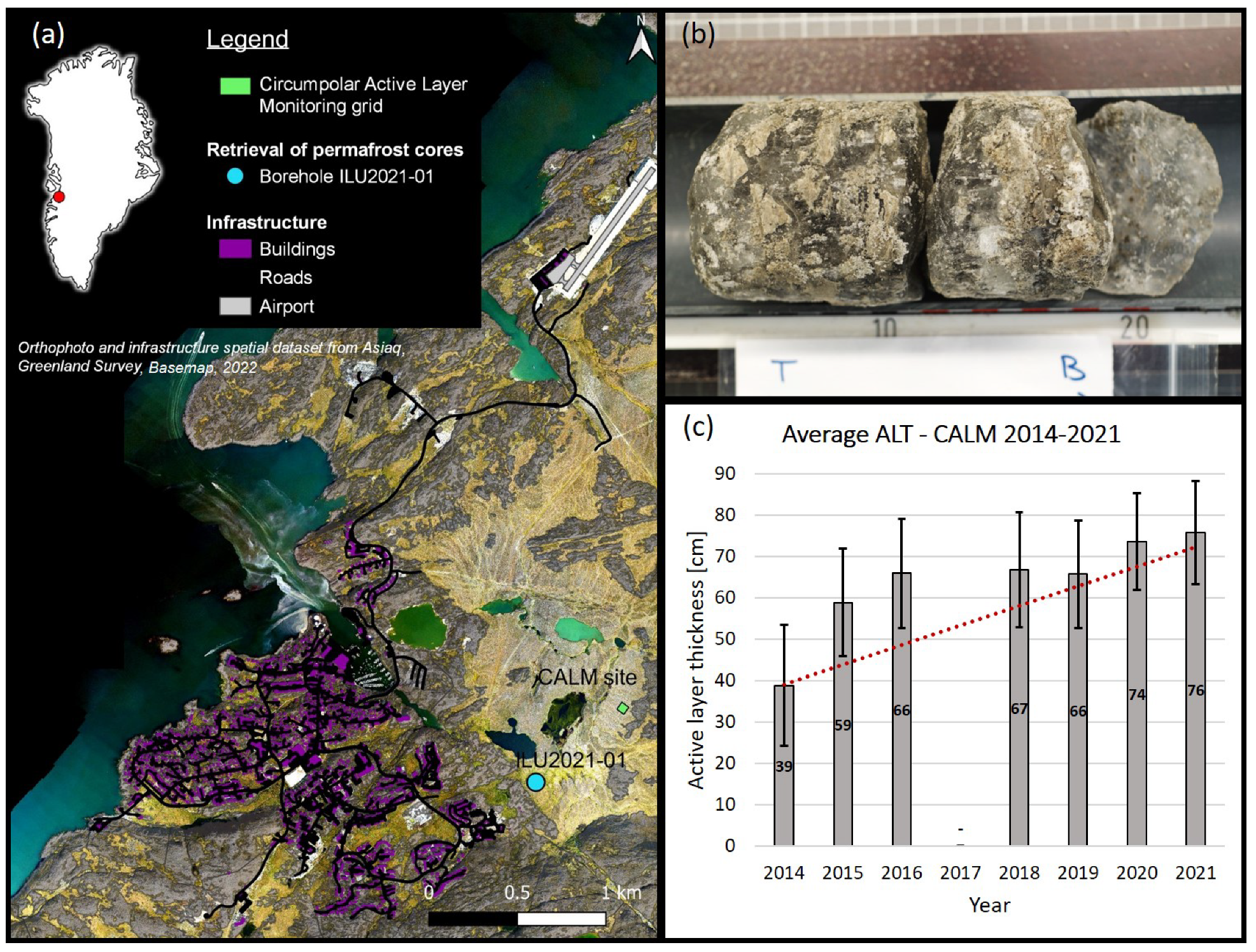ALTs are highly variable spatially, ranging from 30 $\mathrm{cm}$ to more than 2 $\mathrm{m}$, and follow an increasing trend (Figure 1c). During the Holocene deglaciation, fine-grained marine sediments were deposited as a result of marine transgression. The sedimentary deposits gradually became subaerial and exposed to precipitation and percolation due to isostatic uplift. Very ice-rich material (Figure 1b), depleted of salts, is typically found at the permafrost table today. The ground ice content decreases with depth as the pore water salinity increases [32], and for these reasons, permafrost is highly sensitive to climatic changes and surface disturbances.

The landscape is characterized by the presence of these fine-grained marine deposits, lying between gentle bedrock outcrops and interspersed with a system of lakes and small drainage channels. Periglacial features are relatively homogeneous across the area and are primarily dominated by frost boils, which are indicative of the presence of frost-susceptible sediments [25]. Natural water drainage channels and microtopographic depressions form mire zones, becoming wet to inundated during the thawing season, and are colonized by graminoids, bryophytes, and low Salix shrubs. In contrast, frost boil patches are vegetated by dwarf-shrub cryptogam tundra or remain mainly barren, being more exposed to winds.

In this scenery, bedrock outcrops often offer a stable substrate for construction. However, roads and other linear infrastructure extending through sedimentary basins tend to be more heavily affected by seasonal frost/thaw surface deformations and permafrost thaw-induced damages.

Figure 1. Study area and local permafrost conditions. (a) Map of Ilulissat (69.2198${}^{\circ }$ N, 51.0986${}^{\circ }$ W) town area. The map contains an orthophoto and infrastructure spatial data from Asiaq, Greenland Survey, Basemap, 2022 [33]. (b) Permafrost core retrieved in the main sedimentary basin, showing ice-rich fine-grained sediments. (c) Temporal evolution in average active layer thicknesses (ALT), measured at the Ilulissat Circumpolar Active Layer Monitoring (CALM) grid. The red dotted line represents the linear increase in the annually averaged ALT.

Figure 1. Study area and local permafrost conditions. (a) Map of Ilulissat (69.2198${}^{\circ }$ N, 51.0986${}^{\circ }$ W) town area. The map contains an orthophoto and infrastructure spatial data from Asiaq, Greenland Survey, Basemap, 2022 [33]. (b) Permafrost core retrieved in the main sedimentary basin, showing ice-rich fine-grained sediments. (c) Temporal evolution in average active layer thicknesses (ALT), measured at the Ilulissat Circumpolar Active Layer Monitoring (CALM) grid. The red dotted line represents the linear increase in the annually averaged ALT.

3. Materials and Methods

The methodology applied in this study included two main steps outlined in Figure 2. The first step consisted of processing SAR scenes from 2015 to 2019 and modeling InSAR thaw season displacements to retrieve seasonal and long-term trends from the remotely sensed signal (left side of the flowchart in Figure 2). Secondly, we assumed the average seasonal displacement measured by InSAR to be related to the ALT and amount of melted ice in the AL. Statistical–empirical relationships between in situ ALT measurements and surface characteristics (land cover and topography) were investigated with the aim of extrapolating ALT over the study area (methods A and B in Figure 2). The average seasonal displacement and up-scaled ALT were finally used as inputs in our model to estimate the amount of ice present in the AL (right side of the flowchart in Figure 2), which serves as an indicator of the frost susceptibility of the ground.

3.1. Surface Displacement Model

3.1.1. InSAR Observations and Generation of Ground Surface Displacement Maps

Ground surface displacement can be measured and mapped from two SAR images, acquired at different times over the same area, by calculating interferograms of the phase difference between the radar signals. With the aim of mapping ground displacements over the study area, available L1 Single Look Complex Data (SLC) scenes from the ESA/Copernicus Sentinel-1 Constellation were acquired between May and September, spanning thawing seasons from 2015 to 2019. Acquisitions were available following a 6-to-12-day revisit-cycle schedule. Repeat pass interferometry was used on interferometric wide-swath acquisition mode (IW-Mode), which is optimized for interferometric processing.

GAMMA software [34] was used to perform the interferometric processing chain consisting of the co-registration of the images to a common master scene, generation of the interferograms via multi-baseline InSAR [6] and geocoding to a nominal resolution (pixel spacing) set to 10 $\mathrm{m}$. For the orbital correction, geocoding, and interferometric modeling, surface elevation information from the ArcticDEM [35] was used. Short temporal intervals of 12 days in 2015 and 2016, and 6 days since 2017, were mostly picked for the creation of the interferograms. Short intervals were specifically chosen in order to account for the spatial heterogeneity of AL surface deformations and to prevent drops of coherence, typically observed over low-land permafrost areas with pronounced subsidence and significant changes in vegetation and soil moisture conditions, notably at the beginning of the thawing season. In the few cases of missing acquisitions, 24- and 12-day temporal intervals were considered. After removing the topographic, tropospheric and residual geometric phases [6], the interferograms were unwrapped with a minimal cost-flow approach [36] within masked areas using coherence thresholds above 0.8 for spatially filtered and above 0.6 for unfiltered interferograms. During this process, a point located on bedrock (69.2295${}^{\circ }$ N, 51.0184${}^{\circ }$ W) and in close vicinity of the main sedimentary basins was taken as reference. The aforementioned reference point was assumed to be relatively stable with respect to the observed subsidence of the adjacent sedimentary basins and considering that other locations on bedrock did not show deformation.

Although ground thaw begins in early May in Ilulissat, parts of the area may still be snow-covered. In order to avoid de-correlation and phase anomalies from the snow cover, SAR scenes acquired from October to May were removed from the stacks. Gaps that resulted from de-correlated scenes had to be filled by bridging interferometric pairs that would form coherent interferograms again. This implies that the onset of thawing may not be covered by the temporal InSAR stack and is thus not included in the time series of total cumulative displacement. As a result, the displacement is underestimated [20,23], and corrections need to be applied. Offset correction based on Accumulative Degree Days of Thawing (ADDT) has been suggested and demonstrated as applicable [20].

The temporal InSAR stacks of the unwrapped interferograms were finally used to calculate time series of the total cumulative displacements on an annual basis (sign convention positive up, meaning that subsidence is negatively valued). Raster maps of thaw season surface displacement amplitude were generated by taking the maximum cumulative displacement (minimum negative value) observed in the time series at each pixel location. Rasters of thaw season surface displacements were finally converted from radar line-of-sight (LOS) to vertical displacements, using a correction factor of 1.27, which accounts for incidence and elevation angles.

3.1.2. Modeling Approach

At the onset of the thaw season, the active layer is fully frozen. As the soil starts to thaw (Figure 3), the AL progressively deepens (dH). Melting of the ice in the AL gives rise to volume changes and associated subsidence ($\delta$), until the AL has finally reached its maximum thickness (referred to in our paper as the ALT or H). Assuming surface deformations are caused exclusively by pore water phase changes in the soil column, and that lateral exchanges of water do not occur, the total subsidence reached at the end of one thaw season (${\delta }_{max}$) can be correlated to the amount of ice melted. The latter consists of ice formed during the previous year’s winter freeze-up of the AL and possibly ice contained in the transient layer at the top of permafrost, in the case of permafrost degradation.

Liu et al. [16] formulated the following relationship based on the vertical distribution of the pore water in the AL:

$$\delta \left(t\right)={\int }_0^{H\left(t\right)}\varphi ·S_r·\frac{{\rho }_w-{\rho }_i}{{\rho }_i}dH=\varphi ·S_r·\frac{{\rho }_w-{\rho }_i}{{\rho }_i}·H\left(t\right),$$

(1)

where $\delta \left(t\right)$ ($\mathrm{m}$) is the subsidence at time t ($\mathrm{s}$) (with t spanning from the onset of thawing to the time of maximum ALT), $H\left(t\right)$ ($\mathrm{m}$) is the thaw depth at time t, dH ($\mathrm{m}$) is the incremental thickness of thawed soil column, $\varphi$ (-) is the soil porosity, $S_r$ (-) is the total soil water saturation, ${\rho }_w$ ($\mathrm{g}/{\mathrm{cm}}^3$) is the density of pure water, and ${\rho }_i$ ($\mathrm{g}/{\mathrm{cm}}^3$) is the density of ice.

The porosity and saturation could be variable with depth but are considered constant in our analysis, i.e., the ice content is considered homogeneous throughout the AL.

As further evidenced by Liu et al. [16], when measuring surface deformations by InSAR over several thaw seasons, the total measured displacement can be modeled as the combination of an average seasonal component, S, and a long-term displacement rate, R (Figure 3). The seasonal component S is assumed to be representative of surface heave and subsidence induced by freezing and thawing of the AL and the associated ice/water phase and volume changes. The long-term rate is related to changes in the depth of the permafrost table—shallowing or deepening in the case of permafrost aggradation or degradation, respectively. The magnitude of the seasonal component S is consequently strongly correlated with the ice content in the frozen AL and therefore to the frost susceptibility of the soil material. On the other hand, the long-term change component R is related to the ice content at the top of the permafrost (Figure 3).

3.1.3. Adjustment for Partial Temporal Coverage

As previously mentioned, InSAR-measured thaw season surface displacements may not span the entire thawing seasons (Figure 4) and therefore may need adjustment for any additional settlements occurring outside the time span of the temporal InSAR stacks (cf. Section 3.1.1).

The Stefan equation [37] is an analytical solution originally developed to describe sea ice formation, later applied to the freezing of soils by Berggren [38] and to the estimation of thaw depths by, e.g., Hinkel and Nicholas [39]. Widely used as a first approximation, the thaw depth at time t, $H\left(t\right)$, may be estimated using the Stefan equation as follows:

$$H\left(t\right)=\alpha ·\sqrt{\mathrm{ADDT}\left(\mathrm{t}\right)},$$

(2)

where $\alpha$ is a quasi-constant, depending on the thermal properties of the thawed soil, and ADDT is the accumulated degree days of thawing (${}^{\circ }\mathrm{C}·\mathrm{day}$). The ADDT is a time-temperature integral calculated in practice by summing average daily temperatures [40]:

$$\mathrm{ADDT}\left(t\right)=\sum _{i=t_1}^t\overline{T_i}·1\mathrm{day},t_1\le t\le t_2,$$

(3)

where t is an integer representing the day of the year, $t_1$ and $t_2$ represent the start and end of the thawing season (Figure 4), and $\overline{T_i}$ (${}^{\circ }\mathrm{C}$) is the average temperature on day i.

Based on Equation (1) and assuming the relationship in Equation (2) is valid, the surface deformation at any time t is proportional to the square root of ADDT(t).

$$\delta \left(t\right)\sim \sqrt{\mathrm{ADDT}\left(\mathrm{t}\right)}.$$

(4)

In our case, ADDT time series were computed from daily averages of air temperature records [30] and are normalized such that the maximum value is one at the end of the thawing season:

$$\frac{\delta \left(t\right)}{\delta \left(t_2\right)}=\frac{H\left(t\right)}{H\left(t_2\right)}=\sqrt{\frac{\mathrm{ADDT}\left(t\right)}{\mathrm{ADDT}\left(t_2\right)}}=\sqrt{\mathrm{NADDT}\left(t\right)},$$

(5)

resulting in, hereinafter,

$$\delta \left(t\right)=\delta \left(t_2\right)·\sqrt{\mathrm{NADDT}\left(t\right)},t_1\le t\le t_2,$$

(6)

where $\delta \left(t\right)$ ($\mathrm{m}$) and $H\left(t\right)$ ($\mathrm{m}$) are, respectively, the surface deformation and thaw depth at time t, ${\delta }_s\left(t_2\right)$ ($\mathrm{m}$) and $H\left(t_2\right)$ ($\mathrm{m}$) are, respectively, the maximum surface deformation and maximum thaw depth reached at time $t_2$ (the end of the thawing season). $\mathrm{NADDT}\left(t\right)$ is the normalized accumulated degree days of thawing (-).

Using Equation (6), we describe the partial thaw season surface displacement obtained from the temporal InSAR stack by:

$$\Delta {\delta }_s={\delta }_s\left(t_b\right)-{\delta }_s\left(t_a\right)=\delta \left(t_2\right)·\left(\sqrt{\mathrm{NADDT}\left(t_b\right)}-\sqrt{\mathrm{NADDT}\left(t_a\right)}\right),$$

(7)

where $\Delta {\delta }_s$ ($\mathrm{m}$) is the partial thaw season surface displacement observed between time $t_a$ and $t_b$ (time of acquisition of the first and last SAR scene used in the temporal stack, represented as integer day-of-year), subscript s represents values obtained from the InSAR analysis, $\delta \left(t_2\right)$ ($\mathrm{m}$) represents the actual maximum thaw season displacement, which is reached at the end of the thawing season (time $t_2$), and $NADDT\left(t_a\right)$ (-) and $NADDT\left(t_b\right)$ (-) are normalized ADDT at time $t_a$ and $t_b$.

The corrected total thaw season displacement, D ($\mathrm{m}$), is finally derived as:

$$D=\delta \left(t_2\right)=\frac{\Delta {\delta }_s}{\sqrt{\mathrm{NADDT}\left(t_b\right)}-\sqrt{\mathrm{NADDT}\left(t_a\right)}}.$$

(8)

3.1.4. Inversion Methodology

To model the thaw season surface displacement, we use the following relationship:

$$D_i=\left(R·d{Y}_i+S\right),$$

(9)

where $D_i$ ($\mathrm{m}$) is the total thaw season surface displacement in year i, S ($\mathrm{m}$) is the average seasonal displacement over the period of study (the seasonal component), and R ($\mathrm{m}/\mathrm{yr}$) is the average rate of increase in surface displacement amplitude over the period of study. $d{Y}_i$ is the time span (in decimal years) from year i to the midpoint of the InSAR dataset and is calculated as:

$$d{Y}_i=y_i-\frac{y_0+y_N}{2},$$

(10)

where $y_0$ and $y_N$ are, respectively, the first and last year in the InSAR dataset, and $y_i$ represents the integer value of year i.

For multiple years of observations, this constitutes a set of linear equations expressed as follows:

$$\left[\begin{array}{c}{D}_{1,1}\\ ⋮\\ D_{N,1}\\ ⋮\\ D_{1,P}\\ ⋮\\ D_{N,P}\end{array}\right]=\left[\begin{array}{ccccc}d{Y}_1& 1& \cdots & 0& 0\\ ⋮& ⋮& & ⋮& ⋮\\ d{Y}_N& 1& \cdots & 0& 0\\ ⋮& ⋮& \ddots & ⋮& ⋮\\ 0& 0& \cdots & d{Y}_1& 1\\ ⋮& ⋮& & ⋮& ⋮\\ 0& 0& \cdots & d{Y}_N& 1\end{array}\right]·\left[\begin{array}{c}{R}_1\\ S_1\\ ⋮\\ R_P\\ S_P\end{array}\right],$$

(11)

where N is the number of seasons/years in the InSAR temporal stack, and P is the number of pixels in the dataset. Finally, in matrix notation, the system of equations may be reduced to:

$$D=M·RS,$$

(12)

where D is the vector of yearly observed thaw season displacement for every pixel (corrected for partial coverage using Equation (8)), M is the model matrix of time spans and ones, and $RS$ is the vector of R and S parameters per pixel.

We finally solved Equation (9) for R and S using a constrained linear least squares inversion. The seasonal component S was constrained to negative values only, using a modified version of the non-negativity-constrained linear least squares algorithm by Bro and De Jong [41]. The long-term rate R, on the other hand, was allowed to take either negative or positive values depending on the permafrost evolution trends of the area.

The available InSAR dataset was limited to five years, and relatively few data were available to constrain the estimates of R and S for each pixel. To reduce noise, we chose to include information from neighboring pixels in the inversion of R and S for each pixel, effectively representing a spatial smoothing of the parameter estimates. This was carried out by augmenting the system of linear equations with a set of constraining equations as follows:

$$\left[\begin{array}{c}D\\ O\end{array}\right]=\left[\begin{array}{c}M\\ K\end{array}\right]·RS,$$

(13)

where K is a matrix of constraints, with each row representing the constraint of the R or S parameter of one pixel to the R or S parameter of another pixel. O is a vertical vector of zeros with the same number of elements as there are rows in K.

In practice, a 7 × 7 pixel moving window was used, and each pixel was constrained to the 48 surrounding pixels. After inversion, only the parameters derived for the center pixel were stored, and the window was moved to the center on the next pixel. A land cover mask (cf. Section 3.2.2) was used to exclude non-vegetated pixels from the moving window to limit the inversion to sedimentary deposits. In order to assess the least-squares inversion’s performance, the coefficient of determination ($R^2$) was computed for each pixel by calculating the residual sum of squares and total sum of squares, based on the information from the pixels included in the inversion window.

3.1.5. Ice Content Estimation and Frost Susceptibility Index

Compared to geotechnical investigations, ALT measurements are cost and time effective, especially when conducted in the close surroundings of Arctic settlements. For this reason, by taking the reverse approach to that of Liu et al. [16] and Schaefer et al. [24], we estimated the AL ice content at the end of one thawing season by using ALT measurements and the average seasonal displacement (S). Our model therefore assumes homogeneous soil properties and ice content within the AL and at the top of permafrost. Based on Equation (1), we estimated the average AL ice content at each pixel location over the period of study as follows:

$$\varphi ·S_r=\frac{{\rho }_i}{{\rho }_w-{\rho }_i}·\frac{\mid S\mid }{H},$$

(14)

where $\varphi$ (-) is the soil porosity, $S_r$ (-) is the total soil water saturation, and ${\rho }_i$ ($\mathrm{g}/{\mathrm{cm}}^3$) is the density of ice, ${\rho }_w$ ($\mathrm{g}/{\mathrm{cm}}^3$) is the density of liquid water. On a pixel-by-pixel basis, S ($\mathrm{m}$) is the average seasonal displacement measured by InSAR over the period of study 2015–2019, and H ($\mathrm{m}$) is the active layer thickness. Based on prior site investigations conducted in the area, fully saturated soil conditions can generally be assumed ($S_r\approx 1$) at the onset of winter freezing [32], and we assume this to be true throughout the winter until the onset of thawing. The term $\varphi ·S_r$ thus reflects the average AL ice content estimated from the surface deformation caused by the thawing of the AL, assuming no lateral water exchange.

Finally, since the frost susceptibility of a soil is related to its proneness to build up segregated ice, we used the AL ice content as a proxy to map the frost susceptibility of the ground at the community scale. The derived frost susceptibility index, FSI, therefore corresponds to the value of the product:

$$FSI=\varphi ·S_r.$$

(15)

3.2. Data Collection and Processing

Several studies, e.g., [42,43,44,45,46,47], demonstrated the influence of topography and environmental factors (hydrology, vegetation cover, landforms, snow cover) on ALT. Vegetation first strongly influences the surface energy balance, snow cover, soil moisture, and organic content [47]. Vegetation composition and canopy height may consequently provide valuable information on permafrost properties and ALT [42]. In addition, biophysical and physiological properties of plants confer singular spectral reflectance signatures to distinct vegetation units [48]. Topography and microtopography secondly influence vegetation distribution and snow accumulation. As demonstrated in previous studies [43,45,49,50], terrain attributes can therefore be used as an alternative or complement to land cover maps to extrapolate ALT.

Both optical and radar satellite data have been tested for statistical and empirical relationships [15]. They were notably used to model ALT based on correlations with surface characteristics, e.g., [43,44,45,47,51]. We therefore investigated the spatial distribution of ALT and its relationship with vegetation and topographic variables derived from remote sensing. Based on established correlations, ALT measurements conducted over the study domain were extrapolated and finally used as inputs in Equation (14) to estimate the AL ice content and to derive FSI values. We finally validated the InSAR displacement and FSI maps with geotechnical data collected during the study period.

3.2.1. Ground Truth Data

Active Layer Thicknesses

Active layer probing was undertaken every year from 2015 to 2021 (except for 2017) at Ilulissat’s Circumpolar Active Layer Monitoring (CALM) site. The CALM site is a 50 × 50 m grid of 111 points located in a homogeneous zone of frost boils dominated by cryptogams and dwarf shrubs. ALT was additionally measured in 2020 and 2021 at 36 locations spread across the study area. In order to better understand the influence of surface characteristics on the ALT distribution, six transects crossing different landforms and vegetation units were probed in 2020 and 2021. AL probing was always conducted at the end of thawing seasons (when the AL had reached its maximum) with a 110 cm graduated metal rod (ALT probe). The measurement was generally repeated from two to five times at each location, and the values were averaged. The accuracy of the measurements is on the order of 1 cm.

In order to preserve the greatest number of observations, ALT locations that had been exclusively measured in 2021 were recalculated for 2020. To this end, a linear regression was fitted on measurements undertaken both in 2020 and 2021 (Figure 5). In the rest of the paper, we refer to this dataset as ${\mathrm{ALT}}_{20/21}$.

Finally, points located at the transition between distinct vegetation units were discarded from the analysis to reduce ambiguity. A resulting dataset of 335 points was used in the further analysis.

Floristic Surveys and Surface Characteristics

As a way to map local vegetation, floristic surveys were conducted at distributed locations and concurrently along ALT transects. Due to time constraints, the floristic composition (species identification) and Braun–Blanquet (BB) indices of abundance–dominance [52,53] were assessed only once per surveyed homogeneous vegetation unit. At each location, the vegetation was photographed and sampled within a 20 by 20 cm quadrat (September 2020) or 50 by 50 cm quadrat (September 2021). BB indices were converted to percent cover for each of the main plant functional types (PFT) [54], categorized as: non-vegetated (NV), shrubs (S), graminoids (G) including the subcategories grasses (GG), tussock sedges (GTS), non-tussock sedges (GS) and rushes (GR), forbs (F), bryophytes (B), lichens (L) and pteridophytes (P) (Figure A2, Appendix A.2). Periglacial and geomorphological features were described at each survey location, and surface drainage conditions were qualitatively assessed with a scale ranging from very dry to partly inundated.

Agglomerative hierarchical clustering (AHC) using Ward’s method [55,56] was applied to regroup survey locations based on their similarities in PFT percent cover. Clustered data were depicted with a dendogram and plotted in a 2D space using the non-metric multidimentional scaling (NMDS) ordination method [57,58] (Figure A1, Appendix A.1).

Ten main geomorphological and vegetation units, illustrated in Figure 6 and described in

Table 1. Vegetation class descriptions.

Vegetation Class Abbreviation	Description
SLST	Salix-dominated low shrub tundra
EBDST	Empetrum and Betula-dominated dwarf shrub tundra
BSBFB	Betula shrub-dominated, partially bare frost boils
BSVFB	Betula shrub-dominated vegetated frost boils
BSFB	Betula shrub-dominated frost boils
SGCBFB	Shrub, graminoid and cryptogam-dominated, partially bare
	frost boils
SGCVFB	Shrub, graminoid and cryptogam-dominated vegetated frost
	boils
SGCFB	Shrub, graminoid and cryptogam-dominated frost boils
LBFB	Lichen-dominated, partially bare frost boils
LVFB	Lichen-dominated vegetated frost boils
TSGT	Tussock sedge-dominated graminoid tundra
BRSGT	Bryophyte, rush and sedge-dominated graminoid tundra
GGT	Grass-dominated graminoid tundra
SGBT	Shrub, graminoid and bryophyte-dominated tundra

, were identified based on the clustering results and knowledge of the area.

Geotechnical Data

Site investigations were conducted in Ilulissat at 24 locations from 2016 to 2021. Drilling operations, retrieval of soil material, and installation of thermistor strings were notably undertaken in August 2016 and 2018 and in April 2021.

Ground temperatures (GT) were recorded at seven borehole locations established in 2016. As part of the SAR scene processing, GT time series were used to determine the onsets and ends of the thawing seasons. In situ observations showed that the AL typically starts to thaw in May and that the maximum thaw depth (ALT) is reached before or at the onset of freezing (mid-August). Based on this information, the InSAR time series of total cumulative displacements could be adjusted to the actual evolution of the thaw front. The timing of maximum AL development and maximum thaw season displacement were thereby well aligned. GT records were secondarily used to assess the performance of the surface displacement model (based on the Stefan equation), in reproducing the progression of the thaw front depth.

Soil classification experiments and laboratory analyses were conducted on AL samples and permafrost cores in order to validate S, R, and FSI maps [59]. As described in Chamberlain [13], the most common criteria used to evaluate the frost susceptibility of soils rest upon the characterization of particle size. The frost susceptibility classification system developed by Berg and Johnson [60] consists of (i) the determination of the soil type according to the Unified Soil Classification System (USCS) [61], (ii) percentage of particles finer than 0.02 $\mathrm{mm}$, (iii) and laboratory frost heave testing. The ice content, porosity, grain size distribution, and Atterberg plasticity limits were therefore determined on samples collected within the first three meters below the ground surface (AL and top of permafrost). Using the grain size distributions and Atterberg plasticity limits, the samples were then classified based on the USCS [61]. Frost heave experiments were not conducted as part of this study. The frost groups of the samples were finally derived from determined soil properties based on the frost susceptibility classification system mentioned hereinabove [60].

3.2.2. Geospatial Dataset and Environmental Predictors

Vegetation

In our study, spectral information was derived from pre-processed multi-temporal Sentinel-2 bands, acquired during the summers of 2016 and 2017 and resampled to 10 m spatial resolution (

Table 2. Sentinel-2 optical image specifications.

Optical Images	Available Bands	Acquisition Dates	Spatial Resolution
Sentinel-2	B02—BLUE	13 August 2016	10 m
S2A_MSIL2A	B03—GREEN	8 August 2017	10 m
	B04—RED	15 August 2017	10 m
	B05—RED1		20 m
	B06—RED2		20 m
	B07—RED3		20 m
	B08—NIR		10 m
	B08A—NIR2		20 m
	B11—SWIR1		20 m
	B12—SWIR2		20 m

). The spatial resolution differs between the bands. Super-resolution processing (DSen2, [62]) was applied to obtain 10 m for all bands. Further pre-processing steps encompassed sen2cor atmospheric correction, cloud, shadows, snow masking as well as fusion of different image acquisitions (as detailed in [63]). In order to investigate the correlation between spectral data and in situ ALT measurements, several vegetation indices (i.e., normalized difference vegetation index, enhanced vegetation index, etc.), as summarized in

Table A1. List of environmental predictors investigated to spatially extrapolate ALT.

Variable Classes	Abbreviations	Computation Tools or Formulas
Topography
Elevation (m)	DEM	Elevation values from the digital elevation model (DEM) [35]
Slope (degree)	Slope	Tool Slope, Aspect, Curvature, SAGA-GIS [78]
Aspect (degree)	Aspect
Slope height	Slope_height
Mid-slope position	MSP	Tool Relative Heights and Slope Positions, SAGA-GIS [79,80]
Valley depth	Valley_depth
Topographic Position Index	TPI	Tool Topographic Position Index (TPI), SAGA-GIS [81,82,83]
Topographic Wetness Index	TWI	Tool Topographic Wetness Index’ (TWI), SAGA-GIS [78,79]
Accumulated flow	FLOW_D8	Tool Flow Accumulation (Top-Down), deterministic 8 method [78,84,85]
Vegetation
Clay minerals	CLAY_INDEX_SWIR	$SWIR1/SWIR2$
Normalized Difference Vegetation Index	NDVI	$(NIR-RED)/(NIR+RED)$
Green Normalized Difference Vegetation Index	GNDVI	$(NIR-GREEN)/(NIR+GREEN)$
Enhanced Vegetation Index	EVI	$2.5\times (NIR-RED)/(NIR+6\times RED-7.5\times BLUE+1)$
Normalized Difference Water Index	NDWI	$(GREEN-NIR)/(GREEN+NIR)$
Normalized Difference 819/1600 Index	NDII	$(NIR-SWIR1)/(NIR+SWIR1)$
Tasseled Cap—Vegetation	TCV	$-0.2848\times BLUE-0.2435\times GREEN-0.5436\times RED+0.7243\times NIR+0.0840\times SWIR1-0.1800\times SWIR2$
Tasseled Cap—Wetness	TCW	$0.1509\times BLUE+0.1973\times GREEN+0.3279\times RED+0.3406\times NIR-0.7112\times SWIR1-0.4572\times SWIR2$
Principal components	pc1, 2, 3	Principal components from the principal component analysis (PCA) conducted on the ten Sentinel-2 bands

, Appendix B, were firstly derived from the set of ten optical bands.

A principal component analysis (PCA) [64] was performed to remove possibly redundant spectral information in the Sentinel-2 imagery. Concurrently, K-means unsupervised classification [65] was applied to the bands to predetermine the best number of spectral classes to use for the classification process.

Training and validation samples were secondly prepared by extracting representative pixels of non-vegetated and vegetated units within each image band. On average, 80 to 100 pixels were picked for each class of the training dataset, while 40 to 60 were picked for each class of the validation dataset. The previously defined vegetation classes were used to inform the selection process. Spectral distances and signatures of the training samples were computed to ensure sufficient spectral separability between the classes. Classes with low separability were merged, resulting in seven final classes (described in Table 1 and

Table 3. The left column shows vegetation classes originally identified from ground truth data (described in Table 1). To the right, ground-truth classes are regrouped based on their spectral separability and form the final classes used for the classification of the remote-sensing (r-s) data. Cross symbols indicate classes that could not be spectrally distinguished and that were discarded from the classification procedure.

Vegetation Classes	Vegetation Classes
(Ground-Truth)	(r-s Land Cover Classification)
GGT	GGT
TSGT	TSGT
BRSGT	BRSGT
SGBT	X
SLST	X
EBDST	EBDST
BLDST	BLDST
BSBFB	BSFB
BSVFB
SGCBFB	SGCFB
SGCVFB
LBFB
LVFB

).

Different supervised classifiers were finally trained on the training samples and applied to: (i) the three principal components (PC) derived from the PCA, (ii) the set of ten Sentinel-2 image bands, and (iii) the Sentinel-2 bands combined with the PC (13 bands in total). The classification results were individually assessed with the validation dataset by computing the overall accuracy, Kappa coefficient and confusion matrix. The best scores were achieved by using a random forest classifier (RFC) [10,66] on the ten Sentinel-2 bands. Misclassified pixels were reduced by using ancillary data such as elevation and slope rasters presented in the following paragraph. Finally, all non-vegetated classes were merged into one class, representing areas that are not sedimentary deposits in the study area.

Topography

A subset of the ArcticDEM [35], characterized by a spatial resolution of 2 $\mathrm{m}$, was used in this study to derive terrain parameters. Terrain and hydrological variables derived from elevation data were computed in QGIS [67] with SAGA-GIS tools [68] and are summarized in Table A1, Appendix B.

3.2.3. ALT Extrapolation Techniques

Two different methods were tested to extrapolate ALT measurements over the study domain: (A) a statistical model based on relevant predictor variables from among the remotely sensed vegetation and topographic indices; and (B) ALT measurements averaged per vegetation unit and redistributed over the area using the land cover classification raster. The most successful approach was selected to predict and map ALT.

Method A: Statistical Modeling

Hypothesizing that the environmental predictors computed from remote sensing data control the ALT across the study area, we used the ${\mathrm{ALT}}_{20/21}$ as the dependent variable and retrieved the corresponding set of predictor values for each ALT measurement location by sampling the predictor rasters. Correlations between the dependent and predictor variables were then investigated with bivariate regression plots. A reduced subset of predictors appearing correlated with ALT was selected and further investigated.

Due to the limited number of observations ($n=335$), we used a simple generalized linear model (GLM) to predict ALT. Compared to more complex statistical models that may result in overfitting, the GLM is advantageous due to its transparency and interpretability [69,70]. The model, consisting of a multiple linear regression and using topographic and vegetation predictors as inputs, is expressed as follows (Equation (16)) and is fitted by ordinary least squares.

$$y={\beta }_0+{\beta }_1{X}_1+{\beta }_2{X}_2+...+{\beta }_n{X}_n+ϵ,$$

(16)

where y is the predicted ALT ($\mathrm{m}$) (dependent variable), $X_i$ (i varying from 1 to n) are the environmental predictors (independent variables), ${\beta }_i$ (i varying from 1 to n) are the regression coefficients associated with the independent variables, n is the number of independent variables, and $ϵ$ is the model’s error term.

In order to select the best environmental predictors from the subset, a stratified K-fold cross-validation (ten folds) was implemented to assess the model’s predictive performance on all possible combinations of predictors. The Akaike information criterion (AIC) and coefficient of determination ($R^2$) were used as performance metrics. Stratified cross-validation techniques help to randomly split the model’s inputs into training and validation sets while preserving the number of samples in a given class. Here, the land cover classification (cf. Section 3.2.2) was used to ensure an equitable distribution of observations per homogeneous terrain unit.

In our study, multiple environmental predictors were derived from the same data sources (Sentinel-2 images and DEM); therefore, correlations may exist between them. Our final selection was based, on one hand, on the results of the cross-validation (performance metrics), and on the other hand, on bivariate regression plots of the predictors, ensuring a low degree of correlation between the latter. The green normalized difference vegetation index (GNDVI), slope, and flow accumulation (computation detailed in Table A1, Appendix B) were selected as predictors in the final model.

Stratified K-fold cross-validation was lastly repeated (with 5 and 10 folds) to evaluate the final model performance. The average performance of the model was calculated on predictions from all cross-validation test sets.

Method B: Averaging per Vegetation Class

All ALT measurements from the ${\mathrm{ALT}}_{20/21}$ dataset were averaged per vegetation class. In order to assess the significance of the differences between the ALT averages, we performed pairwise statistical t tests. As the distribution of our observations was close to normal, but the size and variance of the class samples were strongly variable, Welch’s t tests were specifically conducted [71]. Finally, averaged ALT values were spatially distributed over the study domain using the land cover classification map. Due to the surface and subsurface conditions, ALT measurements were relatively scarce or unreliable within some of the vegetation units such as EBDST and TSGT (Table 1). In this case, borehole logs and ground temperature records (cf. Section 3.2.1) were used as complementary information to estimate an ALT value for these vegetation units.

4. Results

4.1. InSAR-Derived Surface Displacement Maps

4.1.1. Average Seasonal Displacement and Long-Term Displacement Rate

Figure 7a,b show the derived average seasonal thaw displacement (S) and long-term displacement rate (R) for the study period (2015–2019). Negative values correspond to downward displacement, or in other words, to subsidence of the ground surface. Conversely, positive values indicate surface heave. The average seasonal thaw displacement, S, has a minimum value of −7.5 $\mathrm{cm}$, and S is −2.7 ± 2.0 $\mathrm{cm}$ ($\mu \pm 1\sigma$) on average over the sedimentary areas. R is −0.6 ± 0.5 $\mathrm{cm}/\mathrm{yr}$ and shows a general subsidence of the sedimentary basins. The maximum subsidence rate observed in the area is −2.6 $\mathrm{cm}/\mathrm{yr}$. Our results indicate that permafrost is globally degrading over the study domain, and the ground surface is subsiding due to ice melting near the permafrost table. These observations are supported by AL probing at the CALM site (Figure 1c), which show an increase of around 5 $\mathrm{cm}/\mathrm{year}$ of the AL over the period of study. However, the range of R values obtained (−1 $\mathrm{cm}/\mathrm{year}$ in average) at the same location seems to indicate that the long-term subsidence rate is likely underestimated by our model.

The coefficient of determination ($R^2$), calculated based on the pixels included in the moving window inversion, is mapped in Figure 7c. The $R^2$ was 0.15 ± 0.32 ($\mu \pm 1\sigma$) on average over sedimentary areas (non-vegetated areas excluded). Furthermore, 38.5 and 12.5% of the $R^2$ pixels were larger than 0.25 and 0.5, respectively. The lowest values often occurred in the close vicinity of bedrock, wetlands, surface water, and densely vegetated areas where the InSAR signal may be mixed. Removing pixels located within 50 $\mathrm{m}$ from bedrock increased the average $R^2$ value to 0.25 ± 0.28.

According to the S and R maps, sedimentary deposits in small depressions between bedrock outcrops typically exhibit lower seasonal displacement and long-term subsidence than those observed in larger sedimentary basins (Figure 7a,b). The former areas are usually characterized by relatively dry surface conditions and by the presence of coarse sediments such as sand and stones. In comparison, clays and silts are the most frost-susceptible sediments and expectedly display high S and R values.

Table 4. Comparison of S and R values at borehole locations characterized by different soil types.

Borehole Name	ILU2021-03	ILU16002T	ILU16010T
Dominant AL soil type	SILT	CLAY	SAND
USCS † soil type	ML or MH	CL	SP or SW
S ($\mathrm{m}$)	−0.041	−0.031	−0.016
R ($\mathrm{m}/\mathrm{yr}$)	−0.010	−0.008	−0.003
Ice content below the AL * (%)	80–90	30–40	10–15

† Unified Soil Classification System [61]. * The ice content was visually assessed on permafrost cores retrieved below the permafrost table, based on the Standard Practice For Description Of Frozen Soils [72].

summarizes the S and R values observed at three borehole locations characterized by different soil types.

4.1.2. Assessment of Surface Displacement Model Performance

Our approach to correcting the InSAR-derived subsidence amplitudes is based on a model of AL development as a function of air temperature. In order to assess the ability of our model to reproduce the evolution of the thaw front, we used ground temperature records from seven local boreholes (cf. Section 3.2.1) to calculate time series of the depth of the zero-degree isotherm in 2018 and compared these to the AL evolution modeled with the Stefan equation (Equation (2)). Each time series is normalized to the maximum thaw depth to reduce the dependency on local geological and microclimatic conditions and to mimic the approach taken in the InSAR correction. These time series are illustrated in Figure 8 and show that the onset of thaw is modeled accurately, while the maximum thaw occurs in late August, somewhat earlier than predicted by the model. The discrepancy in the time of maximum thaw depth is inherent to the Stefan equation, which solely takes into account thaw season air temperatures, rather than the full surface energy balance, to predict thaw depths. During most of the thawing season, the model slightly underestimates the normalized thaw depth (by up to 18% in mid-July). This means that the correction factor applied to the InSAR amplitudes is typically underestimated, resulting in conservative estimates of the total thaw season deformations.

4.2. ALT Spatial Distribution and Land Cover

4.2.1. Spatial Variability of Measured ALT

The ALT database compiled as part of this study demonstrated the high spatial and temporal variability of ALT over the study domain, e.g., ALT ranged from 0.30 $\mathrm{m}$ to more than 2 $\mathrm{m}$ in 2020.

At the CALM site, where the vegetation and landforms are homogeneous, ALT measurements conducted from 2015 to 2021 were characterized by standard deviations of 10 to 13 $\mathrm{cm}$ and coefficients of variation of 15 to 20%. However, differences in thaw depths could be identified between distinct vegetation and landform units. Figure 9 illustrates the distribution of ALT along one of the transects probed in 2021 across different terrain units.

Small mounds and terrain patches dominated by higher and denser Betula shrubs (BLDST) were characterized by shallower ALT, in the order of 0.40–0.50 $\mathrm{m}$. Vegetated and partially bare frost boils, colonized by cryptogams (LBFB and LVFB), mixed plant functional types (SGCBFB and SGCVFB), or shrubs (BSBFB and BSVFB) had average ALT between 0.60 and 0.80 $\mathrm{m}$. Finally, the deepest ALT (often more than 1 $\mathrm{m}$) were measured across ponds and natural water drainage channels, which are typically classified as tussock sedges and bryophytes (BRSGT and TSGT). Manual probing and ground temperatures recorded in vegetation units EBDST and TSGT showed that ALT values varied in the approximate range from 1.0 to 2.5 $\mathrm{m}$. These areas are often drier, partially bare or are covered by dwarf shrubs such as Betula nana and Empetrum hermaphroditum (EBDST). These results are generally consistent with ALT measurements conducted in other regions of the Arctic. Rönkkö and Seppälä [73] and Cao et al. [74] both found that a dense and high vegetation cover, notably dominated by low Betula shrubs, may reduce heat losses due to more significant snow accumulation. Rönkkö and Seppälä [73] also reported thicker ALT in the case of drier and coarser soil conditions.

Overall, our observations support the existence of interrelations between the thaw depths, vegetation composition, soil moisture and landforms across the study area.

4.2.2. Supervised Land Cover Classification Results

The overall accuracy of the land cover classification produced by supervised learning from Sentinel-2 optical images was 82.51%, and the Kappa coefficient was 81.40%. At the exception of wetland areas, vegetation units were successfully separated from non-vegetated areas. As illustrated by Figure 10, the spectral signatures of some of the classes were similar. Within non-vegetated classes, many bedrock pixels were erroneously classified as wetlands. Built-up surfaces, gravel, barren areas, and bedrock pixels were also often mistaken. Some of these pixels could nonetheless be reclassified with the help of ancillary data such as topographic indices.

Regrouping vegetation classes according to Table 3 contributed to increasing their spectral distances and separability. However, as expected, vegetation units with resembling species composition and PFT percent cover remained difficult to dissociate. Pixel confusion was considerable for areas covered by a relatively high percentage of shrubs (EBDST, BLDST, BSFB and SGCFB). Similarly, pixels dominated by graminoids and bryophytes were sometimes erroneously divided between the predefined graminoid classes (GGT, BRSGT and TSGT).

4.3. ALT Extrapolation

4.3.1. ALT Extrapolation Based on Method A: Statistical Modeling

Following the approach detailed in Section 3.2.3, we investigated the relationships between the entire ${\mathrm{ALT}}_{20/21}$ dataset and the remotely sensed environmental variables. As a result, the correlations between the ALT and the predictors were found to be weak. The GNDVI, NDVI, OSAVI, slope, mid-slope position, aspect and flow accumulation (Table A1, Appendix B) were slightly correlated to the ALT and were thereby considered the most relevant vegetation and topographic predictors.

A linear regression was firstly fitted onto the ${\mathrm{ALT}}_{20/21}$ and GNDVI data only (Figure 11), for which the highest $R^2$ was obtained (0.10).

Secondly, using the GNDVI, slope, and flow accumulation as inputs in our GLM was still not successful in improving the model performance. Fluctuating and poor cross-validation accuracies ($R^2$ and AIC) were obtained when testing the model on randomly generated training and validation datasets. Even though the respective relationship between the ${\mathrm{ALT}}_{20/21}$ and the predictors was statistically significant (p < 0.05), the model was not able to fit the data and thereby was not representative of the ALT spatial distribution over the entire study domain. Moreover, the GNDVI, which seemed to be the strongest predictor, was inversely correlated to the ${\mathrm{ALT}}_{20/21}$ (Figure 11). This result was in contradiction to ground-truth ALT measurements notably observed over water channels (Figure 9).

The statistical extrapolation of ALT, using a combination of vegetation and topographic indices derived from remote sensing, was not successful in our study area. This method was therefore excluded from predicting ALT and mapping the frost susceptibility.

4.3.2. ALT Extrapolation Based on Method B: Vegetation Classes

Figure 12 presents the average ALT values that were allocated to each vegetation class of the land cover classification raster shown in Figure 13a. The extrapolation procedure resulted in the largest errors for: (i) vegetation classes characterized by an extensive range of ALT values, and (ii) misclassified pixels inherited from the supervised land cover classification (cf. Section 4.2.2). The map in Figure 13b presents the ${\mathrm{ALT}}_{20/21}$ extrapolated over the study domain and used to compute the FSI.

Based on the results of the Welch’s pairwise t tests, the ALT means of most of the vegetation classes were found to be statistically different (p < 0.05). p values superior to 0.05 were obtained when comparing the pairs BSFB-SGCFB, BLDST-GGT, SGCFB-BRSGT and SGCFB-GGT (Table 1), indicating the lack of statistical difference between these classes. The similarity in ALT means of BSFB and SGCFB is inherent to the actual ALT of these frost boil units, although characterized by different floristic compositions. The vegetation class BRSGT often occurs between frost boils or at the transition between distinct land cover units. For this reason, ALT values were significantly variable within this class, and the average ALT turned out to be similar to that of SGCFB. Similarly, few measurements were available for the class GGT, which was also characterized by a wide range in ALT.

Finally, as mentioned in Section 3.2.3, an approximate ALT value of 1.5 $\mathrm{m}$ was attributed to the pixels classified as EBDST. This approximation was used as a proxy to discern areas with the thickest AL, which often correspond to coarse sedimentary deposits (Table 4).

4.4. Frost Susceptibility Index Mapping

Figure 13c shows the FSI derived from extrapolated ALT and S component. The FSI ranges from 0 to 1.7 (unitless).

As a first step toward validating the potential of the FSI, we used AL and permafrost soil properties to assess the frost susceptibility of the ground at different borehole locations (cf. Section 3.2.1). Borehole sites were classified based on the dominant soil type present in the AL or in the first 3 $\mathrm{m}$ below the ground surface. Coarse deposits, categorized as sands (SW and SP in the USCS), gravels and gravel–sand mixtures (GW and GP in the USCS), belong to non-frost susceptible (NFS) to low-frost susceptible soils (S2) according to the United States Army Corps of Engineers Frost Design Soil Classification System (FDSCS) described in Berg and Johnson [60]. These deposits, identified at five borehole locations, were associated with average FSI values of 0.21 ± 0.10 ($\mu \pm 1\sigma$). The rest of the borehole sites were characterized by clays and silts (CL and ML in the USCS). These sediments are highly to very highly frost susceptible (F3–F4) according to the FDSCS [60]. The FSI for this group ranged from 0.14 to almost 0.96, with an average of 0.55 ± 0.25.

Table 5. Comparison of FSI values at borehole locations characterized by different soil types.

Borehole Name	ILU2021-03	ILU16002T	ILU16010T
Dominant AL soil type	SILT	CLAY	SAND
USCS ${}^a$ soil type	ML or MH	CL	SP or SW
FSI (-)	0.63	0.48	0.11
Frost group ${}^b$	F4 ${}^c$	F3 ${}^d$–F4	PFS e–F2 ${}^f$

${}^a$ Unified Soil Classification System [61]. ${}^b$ The frost groups were determined using the US Army Corps of Engineers Frost Design Soil Classification System described in Berg and Johnson [60] based on grain size distribution and Atterberg limits of AL and permafrost samples. ${}^c$ F4 corresponds to very highly frost susceptible soil types. ${}^d$ F3 corresponds to highly frost-susceptible soil types. ^e PFS corresponds to possibly frost-susceptible soil types. ${}^f$ F2 corresponds to moderately frost-susceptible soil types.

shows typical FSI values encountered at borehole locations characterized by different soil types.

As expected, FSI values are higher for fine-grained deposits, suggesting that our approach successfully detected frost-susceptible areas. The degree of frost susceptibility of a given soil type can be relatively broad and controlled by parameters other than the grain size [13]. In addition, the FSI inherited uncertainties and inaccuracies from the processing of the InSAR signal and extrapolation of ALT from the landcover classification. We notably demonstrated that sedimentary deposits surrounded by or located in the close vicinity of bedrock outcrops were subject to poorer inversion performances (Figure 7). These arguments may explain the higher variability of the FSI within sedimentary deposits described as fine-grained (clays and silts).

5. Discussion

5.1. InSAR Surface Displacement Model and Maps

In this study, we modified the algorithm of Liu et al. [8] and applied it to Sentinel-1 SAR scenes acquired between 2015 and 2019. Maps of average seasonal displacement (S) and long-term displacement rate (R) were successfully produced for the community of Ilulissat with a nominal resolution of 10 $\mathrm{m}$. The magnitude of the seasonal deformations was found to be predominantly related to the soil type and moisture conditions. Compared to fine-grained sedimentary deposits that exhibited severe surface displacements, less subsidence was observed in coarser and drier areas. These observations, which were substantiated by soil properties measured at borehole locations [59], corroborate the findings of Schaefer et al. [24]. The R map also highlighted zones of larger downward displacement trends that were interpreted as degrading permafrost areas. Our results generally confirmed the measured increase in AL over the study time frame but underestimated the magnitude of the long-term subsidence.

Overall, our surface displacement model was able to explain up to 25% of the InSAR data variation over the sedimentary basins. The model performance was considerably reduced over high shrubs, inundated areas, and in the close vicinity of bedrock. In their studies, Jia et al. [75], Strozzi et al. [6] and Zwieback and Meyer [14] experienced similar errors characteristic of the use of InSAR over low-land permafrost, densely vegetated, barren, and rocky areas. As discussed by the authors and by Ansari et al. [76], changes in ionospheric, vegetation, and soil moisture conditions exert an influence on radar penetration and may introduce biases in the InSAR signal (notably drop of coherence) and measured surface displacement. This phenomenon partly explains our inversion results and the positive R values specifically observed at a few locations and indicating a decreasing trend in ALT. These areas typically align with wetlands, where ponds and water accumulation may have affected the coherence of the InSAR signal. Anthropogenic modifications may also have resulted in heave or mixed signals in the derived S and R maps at specific locations. Future work could investigate and quantify the impacts of vegetation density and surface drainage conditions on the coherence of the InSAR signal.

The main contribution of our approach lied in the implementation of a moving-windowed constrained linear least-squares inversion. In order to compensate for the lack of points in the temporal InSAR dataset and assuming that spatial variations were smooth, several pixel values were used in the inversion, providing more information from neighboring areas and reducing the noise in the data. However, this technique may not have been sufficient to entirely balance out the fact that only five years of InSAR images could be processed. For this reason, the R component, which represented the “long-term” trend in surface deformations and was interpreted as changes in the permafrost table depth, should still be considered cautiously. The robustness of the inversion and estimation accuracy of the R component could be improved if longer InSAR time series of surface displacements were available, therefore providing more points to constrain the inversion and to reduce the uncertainty in the estimated parameters. The inversion could additionally be weighted based on the land cover classes.

Secondly, the generation of the displacement time series and variations in the temporal coverage of the InSAR stacks (and therefore in the measured thaw season vertical displacement) may have also lessened the inversion capability of our algorithm. Our model notably relied on the Stefan equation to reproduce the evolution of the thaw front. By validating the evolution of the thawing front with ground temperature measurements, we demonstrated that the Stefan approximation is well suited to model the onset of thawing but that predicted thaw depths are somewhat underestimated. The correction factor applied to the InSAR amplitudes was therefore also underestimated, and the final S and R products should thus be considered as conservative estimates. In our dataset, the 2015 time series notably started very late in the thawing season, which may have contributed to a larger variation in the observations and to poorer regression fits. Such effects especially impact relatively short stacks (study periods) such as ours.

In our model, we also assumed that vertical displacements of the ground surface would only be caused by volume changes induced by the freezing and thawing of the AL. Assuming that there were no lateral water exchanges was appropriate for the area of Ilulissat where the topography is flat. Nonetheless, as mentioned by Liu et al. [8,16], secondary driving mechanisms such as erosion, clay contraction, inundation, and other changes in soil properties may contribute to ground movements but were not accounted for in our model.

In comparison, sinusoidal models have been tested by Li et al. [17] and Jia et al. [75] and have generally proved performant. However, many physical processes influencing the occurrence and magnitude of surface deformations do not follow sinusoidal trends [17,75]. Further modeling efforts are required to improve the representation of ground movements occurring in permafrost regions.

The S and R values retrieved from the inversion were assessed against AL and top-of-permafrost soil properties determined at borehole locations. Even though our results were coherent with subsurface conditions at these locations, measurements of the surface displacements are still needed to quantitatively validate seasonal and long-term deformation trends. To this aim, subsidence sticks could be deployed in the study area, as described in Antonova et al. [9] and Bartsch et al. [20].

5.2. ALT Extrapolation Techniques

We investigated the correlations between a set of remotely sensed environmental predictors and ALT probed in 2020 and 2021 (${\mathrm{ALT}}_{20/21}$). Field measurements conducted in Ilulissat evidenced the strong spatial variability of ALT across the study domain. Our observations are in line with previous studies that reported large variations in ALT within study sites across the Arctic, e.g., [16,45,75].

Weak linear correlations were found between ${\mathrm{ALT}}_{20/21}$ and a subset of predictors. Therefore, we first attempted to extrapolate ${\mathrm{ALT}}_{20/21}$ with a GLM whose predictive capability was evaluated by cross-validation. The model performed poorly and was unstable when fitted and validated on randomly generated samples. With this approach, we were not able to reproduce the variability in ALT across the study domain. Other researchers have experienced similar challenges when statistically predicting ALT from geospatial datasets. Karjalainen et al. [12], who used an ensemble model at the pan-Arctic scale, notably reported relatively large uncertainties associated with the predictions of present and past ALT (adjusted $R^2$ of, respectively, 0.37 and 0.57). The geographically weighted regression approach implemented by Mishra and Riley [45] over the state of Alaska was also characterized by a moderate predictive capability.

The poor performance of our model could be attributed to the combination of ALT measurements, predictors, and algorithms selected for this study. Before 2020, ALT measurements were scarce and relatively localized. Averaging ALT values over the study period of 2015–2019 (cf. Equation (14)) was not possible in our case since the dataset would not have been representative of the natural spatial variability of ALT. In order to maximize the spatial distribution of our dataset and the robustness of the extrapolation procedure, ALT measured in 2020 and 2021 was used instead. However, as field protocols changed with our understanding of the area throughout the project, ALT probing was conducted inconsistently across vegetation and landform units in 2020 and 2021. Final sample sizes were therefore larger among certain vegetation classes, while others remained underrepresented. For the same reason, our dataset did not entirely and evenly span the spectrum of values of the environmental predictor rasters, which were sampled at the ALT probing locations only. We recommend that the density and distribution of ALT measurements for validation purposes are carefully considered to appropriately represent different terrain units in future studies.

Furthermore, the area of Ilulissat is characterized by a gentle relief and by homogenous periglacial features (frost boils). Floristic, hydrological, and geomorphological disparities evidently exist, but their spatial gradients are relatively small. Within a homogeneous terrain unit, intra-variations in vegetation composition, soil moisture, microtopography, and ALT additionally occur. However, the resolution of the remotely sensed datasets acquired for this study was likely insufficient in grasping such nuances. Statistical models applied at smaller scales (hundreds of meters) and using high-resolution surface elevation and multi-spectral data were generally successful in predicting ALT [43]. In this context, Anderson et al. [77] showed that hyperspectral imaging can be more suitable in relation to statistical extrapolations. Acquiring predictors with a higher resolution could contribute to improving our ${\mathrm{ALT}}_{20/21}$ predictions.

Finally, a different statistical model could be tested on our datasets, provided that more observations are collected. In our case, a GLM was chosen due to the reduced number of measurements and ease of interpretability [69]. Relationships between the ALT and surface characteristics may not all be linear. For this reason, generalized additive models (GAM), which present the advantage of accounting for non-linear effects, could be a more flexible alternative to the GLM.

To overcome these difficulties, we exploited the correlation between the thaw depths and vegetation zonation revealed by ALT probing along transects. ALT measurement sites were categorized based on their sampled floristic composition and averaged per-spectral vegetation class ensuing from the supervised land cover classification map. This method was substantially more successful and representative of the ALT spatial distribution than the statistical model. Prediction errors were tied to vegetation misclassifications and class intra-variability in ALT. Floristic surveys were conducted relatively late (September) compared to the vegetation growing season peak (mid-July to mid-August). It is plausible that the species richness was not fully captured in our data, but species abundance and PFT percent covers were expected to represent distinct vegetation types. The RFC-supervised algorithm produced satisfactory classification results (82.51% overall accuracy). Nonetheless, vegetation classes identified from ground truth data were not always spectrally separable, resulting in pixel confusion and misclassifications. These errors may have led to the wrong allocation of ALT values in some locations. Lastly, t tests revealed overlaps and statistical similarities in ALT averages computed for two pairs of vegetation classes. These results were coherent with the natural variability of thaw depths measured within these units. Our study confirms the conclusions of Mishra and Riley [45], stating that using vegetation zonation as an indicator of ALT does involve uncertainties but is applicable when more complex statistical models can not be implemented.

The distribution of ALT is influenced by many factors, the relative importance of which is scale-dependent. Previous studies have shown that air temperature is the primary control of ALT over large scales [43]. Land cover types and topography also exert a strong influence on ALT. At microscales, Gangodagamage et al. [43] and Anderson et al. [77] demonstrated that microtopography, vegetation, and soil moisture become predominant driving factors. In our study areas, land cover units proved to be the best predictor of ALT. Due to the lack of strong topographic gradients, the effects of terrain parameters investigated in this study could not be asserted. The significant spatial variability of ALT is still not fully understood. The suitability of different extrapolation techniques and predictors remains considerably site-dependent. More robust approaches that could be extended to different permafrost environments must be developed. Additional monitoring, remote sensing, and modeling efforts remain needed to bridge the gap between micro- and regional scales.

5.3. Frost Susceptibility Mapping

Mapping ground ice traditionally relies on geomorphological expertise and the identification of periglacial features [25]. Using remote sensing techniques would be highly advantageous in Arctic regions where drilling and soil sampling are logistically challenging and costly. However, to this day, the possibilities to derive ice content from remotely sensed signals are limited [14]. Liu et al. [16] were able to link changes in surface subsidence to the thawing of the AL. Using a similar approach, we estimated the AL ice content from 2015 to 2019 average seasonal displacements (S) and extrapolated field observations (${\mathrm{ALT}}_{20/21}$). Since thaw depths follow an increasing trend in Ilulissat, the ${\mathrm{ALT}}_{20/21}$ dataset we applied may be overestimating the ALT averaged over the study period 2015–2019. Referring to Equation (14), we can infer that the resulting AL ice content represents a conservative estimate (underestimated). Furthermore, homogeneous porosity and saturation of the AL had to be assumed. These simplifications and errors intrinsic to the retrieval of the S component and predicted ${\mathrm{ALT}}_{20/21}$ introduced additional uncertainty in our results. We named the final product a frost susceptibility index (FSI) to underpin that it does not represent an exact quantification.

Despite reaching an accurate quantification of the AL ice content, we qualitatively compared obtained FSI values to frost susceptibility classification of sediment samples based on the FDSCS [60]. The frost susceptibility of AL and permafrost samples corroborated the InSAR-derived FSI, thereby supporting the validity of our mapping approach.

Our efforts are presented here as a first step toward developing remote sensing techniques for ground ice retrieval. Further research could consist in investigating the relevance of extreme year analyses [14,20] for our study area. Using late-season subsidence signals to distinguish ice-rich from ice-poor areas proved effective under the following conditions: (i) exceptionally warm summers (ii) and initial melting of excess ice at the top of permafrost. In the case of Ilulissat, the derived R map indicated locations that may be subject to ongoing permafrost degradation. Secondly, 2019 was a particularly warm year, with mean annual air temperature reaching −2 ${}^{\circ }\mathrm{C}$ and thawing degree days exceeding 1000. Testing this method for this year, in particular, could provide complementary information with respect to the localization of vulnerable ice-rich areas.

5.4. Potential of InSAR-Derived Maps to Support Infrastructure Maintenance and Planning

In remote Arctic areas, geotechnical data are relatively rare and challenging to acquire. However, site investigations remain essential to adapt construction practices to permafrost conditions and to prevent failures. In this context, remote sensing techniques provide high-resolution and continuous spatial information that can be validated with relatively reduced ground-truth datasets.

InSAR measurements notably provide insightful information regarding AL dynamics and permafrost degradation where surface deformations severely or repeatedly affect the built environment. Used as a complement to site investigations and local knowledge, InSAR maps, therefore, have the potential to support the construction and planning sectors. Such tools are especially valuable in the context of risk management and Arctic urban sprawl. Possible causes of infrastructure deterioration can first be identified, and maintenance operations be more judiciously prioritized. In this study, we implemented a multidisciplinary mapping framework with the aim to map the frost susceptibility of the ground at the community scale. Our work contributed to identifying hazardous frost-susceptible areas currently subject to large seasonal surface displacements and/or long-term subsidence. FSI maps derived from our approach may secondly be helpful in informing construction planning in unbuilt areas with limited geotechnical data, such as in Ilulissat (Figure 14).

6. Conclusions

We processed Sentinel-1 SAR scenes acquired between 2015 and 2019 to map ground surface displacements over the community of Ilulissat, West Greenland. Average seasonal displacements (S) and long-term subsidence rates (R) were derived from the interferogram stack. Active layer thickness (ALT) measurements were extrapolated using remotely sensed surface characteristics to retrieve a frost susceptibility index. The resulting maps were validated against soil properties. Our main conclusions are listed hereinafter:

• In Ilulissat, fine-grained sedimentary basins were subject to significant downward seasonal deformations of the ground surface during the study period, in the order of 3 to 8 $\mathrm{cm}$. Several locations also seem to follow a subsiding trend in the long term, indicating permafrost degradation and possible melting of excess ice below the permafrost table. Coarse-grained and drier sedimentary deposits were found to be more stable. The surface deformations’ severity generally seemed to be correlated to the soil type and moisture.
• The surface displacement model applied in this study was able to explain up to 25% of the observed data variation over sedimentary basins. Densely vegetated, rocky or inundated areas were subject to a higher degree of uncertainty, likely inherited from anomalies in the InSAR signal. Surface deformation models currently based on the Stefan equation or sinusoidal functions require further research.
• At the micro- and community scales, the distribution of ALT is very variable in Ilulissat, ranging from 0.3 $\mathrm{m}$ to more than 2 $\mathrm{m}$. Despite evident correlations with surface characteristics such as vegetation cover, the extrapolation of ALT measurements was challenging. A statistical model (GLM), using remotely sensed vegetation and topographic parameters as inputs, failed to reproduce the spatial variability of ALT over the entire study area. The density and distribution of ALT measurements, and the spatial resolution of remotely sensed predictors, likely need to be improved to obtain more reasonable predictions. Averaging ALT per vegetation unit and distributing the values over the study domain, based on a supervised land cover classification of Sentinel-2 images, proved to be the most successful technique in our case.
• Extrapolated ALT and average seasonal displacements were used as inputs to derive an indicator of the frost susceptibility of the ground. Although uncertainties inherent to assumptions and inherited errors in ALT and S were associated with the retrieval of the frost susceptibility index (FSI), the latter was in good agreement with soil properties determined from AL and permafrost samples. Locations classified for the presence of fine-grained and coarse sedimentary deposits were respectively characterized by average FSI values of 0.55 and 0.21.
• Our approach enabled us to identify frost-susceptible and ice-rich areas, subject to severe seasonal surface deformations and/or long-term subsidence from degrading permafrost. We demonstrated the potential of InSAR-derived maps in combination with geotechnical information to support infrastructure maintenance and planning in permafrost environments.

References

1. Andersland, O.B.; Ladanyi, B. Frozen Ground Engineering; John Wiley & Sons: Hoboken, NJ, USA, 2003. [Google Scholar]
2. Jorgenson, M.T.; Shur, Y.L.; Pullman, E.R. Abrupt increase in permafrost degradation in Arctic Alaska. Geophys. Res. Lett. 2006, 33. [Google Scholar] [CrossRef]
3. Romanovsky, V.E.; Smith, S.L.; Christiansen, H.H. Permafrost thermal state in the polar Northern Hemisphere during the international polar year 2007–2009: A synthesis. Permafr. Periglac. Process. 2010, 21, 106–116. [Google Scholar] [CrossRef] [Green Version]
4. Doré, G.; Zubeck, H.K. Cold Regions Pavement Engineering; Mcgraw-Hill Education: Berkshire, UK, 2009. [Google Scholar]
5. Shiklomanov, N.I.; Streletskiy, D.A.; Swales, T.B.; Kokorev, V.A. Climate change and stability of urban infrastructure in Russian permafrost regions: Prognostic assessment based on GCM climate projections. Geogr. Rev. 2017, 107, 125–142. [Google Scholar] [CrossRef]
6. Strozzi, T.; Antonova, S.; Günther, F.; Mätzler, E.; Vieira, G.; Wegmüller, U.; Westermann, S.; Bartsch, A. Sentinel-1 SAR interferometry for surface deformation monitoring in low-land permafrost areas. Remote Sens. 2018, 10, 1360. [Google Scholar] [CrossRef] [Green Version]
7. Streletskiy, D.A.; Suter, L.J.; Shiklomanov, N.I.; Porfiriev, B.N.; Eliseev, D.O. Assessment of climate change impacts on buildings, structures and infrastructure in the Russian regions on permafrost. Environ. Res. Lett. 2019, 14, 025003. [Google Scholar] [CrossRef]
8. Liu, L.; Zhang, T.; Wahr, J. InSAR measurements of surface deformation over permafrost on the North Slope of Alaska. J. Geophys. Res. Earth Surf. 2010, 115, F03023. [Google Scholar] [CrossRef]
9. Antonova, S.; Sudhaus, H.; Strozzi, T.; Zwieback, S.; Kääb, A.; Heim, B.; Langer, M.; Bornemann, N.; Boike, J. Thaw subsidence of a yedoma landscape in northern Siberia, measured in situ and estimated from TerraSAR-X interferometry. Remote Sens. 2018, 10, 494. [Google Scholar] [CrossRef] [Green Version]
10. Mohammadimanesh, F.; Salehi, B.; Mahdianpari, M.; English, J.; Chamberland, J.; Alasset, P.J. Monitoring surface changes in discontinuous permafrost terrain using small baseline SAR interferometry, object-based classification, and geological features: A case study from Mayo, Yukon Territory, Canada. GIScience Remote Sens. 2019, 56, 485–510. [Google Scholar] [CrossRef]
11. Hjort, J.; Karjalainen, O.; Aalto, J.; Westermann, S.; Romanovsky, V.E.; Nelson, F.E.; Etzelmüller, B.; Luoto, M. Degrading permafrost puts Arctic infrastructure at risk by mid-century. Nat. Commun. 2018, 9, 5147. [Google Scholar] [CrossRef] [Green Version]
12. Karjalainen, O.; Aalto, J.; Luoto, M.; Westermann, S.; Romanovsky, V.E.; Nelson, F.E.; Etzelmüller, B.; Hjort, J. Circumpolar permafrost maps and geohazard indices for near-future infrastructure risk assessments. Sci. Data 2019, 6, 190037. [Google Scholar] [CrossRef] [Green Version]
13. Chamberlain, E.J. Frost Susceptibility of Soil, Review of Index Tests. Technical report; Cold Regions Research and Engineering Lab: Hanover, NH, USA, 1981. [Google Scholar]
14. Zwieback, S.; Meyer, F.J. Top-of-permafrost ground ice indicated by remotely sensed late-season subsidence. Cryosphere 2021, 15, 2041–2055. [Google Scholar] [CrossRef]
15. Bartsch, A.; Strozzi, T.; Nitze, I. Permafrost Monitoring from Space. Surv. Geophys. 2023, 1–35. [Google Scholar] [CrossRef]
16. Liu, L.; Schaefer, K.; Zhang, T.; Wahr, J. Estimating 1992–2000 average active layer thickness on the Alaskan North Slope from remotely sensed surface subsidence. J. Geophys. Res. Earth Surf. 2012, 117, F01005. [Google Scholar] [CrossRef]
17. Li, Z.; Zhao, R.; Hu, J.; Wen, L.; Feng, G.; Zhang, Z.; Wang, Q. InSAR analysis of surface deformation over permafrost to estimate active layer thickness based on one-dimensional heat transfer model of soils. Sci. Rep. 2015, 5, 15542. [Google Scholar] [CrossRef] [PubMed] [Green Version]
18. Daout, S.; Doin, M.P.; Peltzer, G.; Socquet, A.; Lasserre, C. Large-scale InSAR monitoring of permafrost freeze-thaw cycles on the Tibetan Plateau. Geophys. Res. Lett. 2017, 44, 901–909. [Google Scholar] [CrossRef]
19. Wang, C.; Zhang, Z.; Zhang, H.; Zhang, B.; Tang, Y.; Wu, Q. Active layer thickness retrieval of Qinghai–Tibet permafrost using the TerraSAR-X InSAR technique. IEEE J. Sel. Top. Appl. Earth Obs. Remote Sens. 2018, 11, 4403–4413. [Google Scholar] [CrossRef]
20. Bartsch, A.; Leibman, M.; Strozzi, T.; Khomutov, A.; Widhalm, B.; Babkina, E.; Mullanurov, D.; Ermokhina, K.; Kroisleitner, C.; Bergstedt, H. Seasonal Progression of Ground Displacement Identified with Satellite Radar Interferometry and the Impact of Unusually Warm Conditions on Permafrost at the Yamal Peninsula in 2016. Remote Sens. 2019, 11, 1865. [Google Scholar] [CrossRef] [Green Version]
21. Rouyet, L.; Lauknes, T.R.; Christiansen, H.H.; Strand, S.M.; Larsen, Y. Seasonal dynamics of a permafrost landscape, Adventdalen, Svalbard, investigated by InSAR. Remote Sens. Environ. 2019, 231, 111236. [Google Scholar] [CrossRef]
22. Chen, J.; Wu, Y.; O’Connor, M.; Cardenas, M.B.; Schaefer, K.; Michaelides, R.; Kling, G. Active layer freeze-thaw and water storage dynamics in permafrost environments inferred from InSAR. Remote Sens. Environ. 2020, 248, 112007. [Google Scholar] [CrossRef]
23. Rouyet, L.; Liu, L.; Strand, S.M.; Christiansen, H.H.; Lauknes, T.R.; Larsen, Y. Seasonal InSAR Displacements Documenting the Active Layer Freeze and Thaw Progression in Central-Western Spitsbergen, Svalbard. Remote Sens. 2021, 13, 2977. [Google Scholar] [CrossRef]
24. Schaefer, K.; Liu, L.; Parsekian, A.; Jafarov, E.; Chen, A.; Zhang, T.; Gusmeroli, A.; Panda, S.; Zebker, H.A.; Schaefer, T. Remotely sensed active layer thickness (ReSALT) at Barrow, Alaska using interferometric synthetic aperture radar. Remote Sens. 2015, 7, 3735–3759. [Google Scholar] [CrossRef] [Green Version]
25. Allard, M.; Lemay, M.; Barrette, C.; L’Hérault, E.; Sarrazin, D.; Bell, T.; Doré, G. Permafrost and climate change in Nunavik and Nunatsiavut: Importance for municipal and transportation infrastructures. In Nunavik and Nunatsiavut: From Science to Policy. An Integrated Regional Impact Study (IRIS) of Climate Change and Modernization; ArcticNet Inc.: Quebec City, QC, Canada, 2012; pp. 171–197. [Google Scholar]
26. Short, N.; LeBlanc, A.M.; Sladen, W.; Oldenborger, G.; Mathon-Dufour, V.; Brisco, B. RADARSAT-2 D-InSAR for ground displacement in permafrost terrain, validation from Iqaluit Airport, Baffin Island, Canada. Remote Sens. Environ. 2014, 141, 40–51. [Google Scholar] [CrossRef]
27. Ingeman-Nielsen, T.; Lemay, M.; Allard, M.; Barrette, C.; Bjella, K.; Brooks, H.; Carbonneau, A.S.; Doré, G.; Foged, N.; Lading, T.; et al. Built infrastructure. In Adaptation Actions for a Changing Arctic: Perspectives from the Baffin Bay/Davis Strait Region; Arctic Monitoring and Assessment Programme (AMAP): Oslo, Norway, 2018; pp. 261–306. [Google Scholar]
28. European Commission. Forging a Climate-Resilient Europe—The New EU Strategy on Adaptation to Climate Change; European Commission: Brussels, Belgium, 2021; Available online: https://eur-lex.europa.eu/legal-content/EN/TXT/PDF/?uri=CELEX:52021DC0082&from=EN (accessed on 11 May 2023).
29. Avannaata Kommunia. Byudvikling Ilulissat Nord. 2021. Available online: https://www.avannaata.gl/nyheder/2021/03/31_strukturplan (accessed on 11 May 2023).
30. Cappelen, J. Weather Observations from Greenland 1958–2020. Observation Data with Description; Technical Report 21-08; Danish Meteorological Institute: Copenhagen, Denmark, 2021; Available online: https://www.dmi.dk/fileadmin/Rapporter/2021/DMIRep21-08.pdf (accessed on 11 May 2023).
31. Christiansen, H.H.; Etzelmüller, B.; Isaksen, K.; Juliussen, H.; Farbrot, H.; Humlum, O.; Johansson, M.; Ingeman-Nielsen, T.; Kristensen, L.; Hjort, J.; et al. The thermal state of permafrost in the nordic area during the international polar year 2007–2009. Permafr. Periglac. Process. 2010, 21, 156–181. [Google Scholar] [CrossRef] [Green Version]
32. Tomaškovičová, S.; Ingeman-Nielsen, T. Quantification of freeze-thaw hysteresis of unfrozen water content and electrical resistivity from time lapse measurements in the active layer and permafrost. Permafr. Periglac. Process. 2023, submitted.
33. Asiaq Greenland Survey. Asiaq Map Supply Service. 2022. Available online: https://kortforsyning.asiaq.gl/ (accessed on 11 May 2023).
34. Werner, C.; Wegmüller, U.; Strozzi, T.; Wiesmann, A. Gamma SAR and interferometric processing software. In Proceedings of the Ers-Envisat Symposium, Gothenburg, Sweden, 16–20 October 2000; Volume 1620, p. 1620. [Google Scholar]
35. Porter, C.; Morin, P.; Howat, I.; Noh, M.J.; Bates, B.; Peterman, K.; Keesey, S.; Schlenk, M.; Gardiner, J.; Tomko, K.; et al. ArcticDEM, Version 3. 2018. Available online: https://www.pgc.umn.edu/data/arcticdem/ (accessed on 11 May 2023). [CrossRef]
36. Costantini, M. A novel phase unwrapping method based on network programming. IEEE Trans. Geosci. Remote Sens. 1998, 36, 813–821. [Google Scholar] [CrossRef]
37. Stefan, J. Über die Theorie der Eisbildung, insbesondere über die Eisbildung im Polarmeere. Ann. Phys. 1891, 278, 269–286. [Google Scholar] [CrossRef] [Green Version]
38. Berggren, W. Prediction of temperature-distribution in frozen soils. Eos Trans. Am. Geophys. Union 1943, 24, 71–77. [Google Scholar] [CrossRef]
39. Hinkel, K.M.; Nicholas, J.R. Active layer thaw rate at a boreal forest site in central Alaska, USA. Arct. Alp. Res. 1995, 27, 72–80. [Google Scholar] [CrossRef]
40. Lunardini, V.J. Heat Transfer in Cold Climates; Van Nostrand Reinhold Company: New York, NY, USA, 1981. [Google Scholar]
41. Bro, R.; De Jong, S. A Fast Non-negativity-Constrained Least Squares Algorithm. J. Chemom. 1997, 11, 393–401. [Google Scholar] [CrossRef]
42. Duguay, C.R.; Zhang, T.; Leverington, D.W.; Romanovsky, V.E. Satellite remote sensing of permafrost and seasonally frozen ground. Geophys. Monogr.-Am. Geophys. Union 2005, 163, 91. [Google Scholar]
43. Gangodagamage, C.; Rowland, J.C.; Hubbard, S.S.; Brumby, S.P.; Liljedahl, A.K.; Wainwright, H.; Wilson, C.J.; Altmann, G.L.; Dafflon, B.; Peterson, J.; et al. Extrapolating active layer thickness measurements across Arctic polygonal terrain using LiDAR and NDVI data sets. Water Resour. Res. 2014, 50, 6339–6357. [Google Scholar] [CrossRef] [Green Version]
44. Li, A.; Tan, X.; Wu, W.; Liu, H.; Zhu, J. Predicting active-layer soil thickness using topographic variables at a small watershed scale. PLoS ONE 2017, 12, e0183742. [Google Scholar] [CrossRef] [PubMed]
45. Mishra, U.; Riley, W.J. Active-layer thickness across Alaska: Comparing observation-based estimates with CMIP5 Earth system model predictions. Soil Sci. Soc. Am. J. 2014, 78, 894–902. [Google Scholar] [CrossRef] [Green Version]
46. Nelson, F.; Shiklomanov, N.; Mueller, G.; Hinkel, K.; Walker, D.; Bockheim, J. Estimating active-layer thickness over a large region: Kuparuk River basin, Alaska, USA. Arct. Alp. Res. 1997, 29, 367–378. [Google Scholar] [CrossRef]
47. Pastick, N.J.; Jorgenson, M.T.; Wylie, B.K.; Minsley, B.J.; Ji, L.; Walvoord, M.A.; Smith, B.D.; Abraham, J.D.; Rose, J.R. Extending airborne electromagnetic surveys for regional active layer and permafrost mapping with remote sensing and ancillary data, Yukon Flats Ecoregion, Central Alaska. Permafr. Periglac. Process. 2013, 24, 184–199. [Google Scholar] [CrossRef] [Green Version]
48. Laidler, G.J.; Treitz, P. Biophysical remote sensing of arctic environments. Prog. Phys. Geogr. 2003, 27, 44–68. [Google Scholar] [CrossRef]
49. Peddle, D.R.; Franklin, S.E. Classification of permafrost active layer depth from remotely sensed and topographic evidence. Remote Sens. Environ. 1993, 44, 67–80. [Google Scholar] [CrossRef]
50. Gao, T.; Zhang, T.; Wan, X.; Kang, S.; Sillanpää, M.; Zheng, Y.; Cao, L. Influence of microtopography on active layer thaw depths in Qilian Mountain, northeastern Tibetan Plateau. Environ. Earth Sci. 2016, 75, 382. [Google Scholar] [CrossRef]
51. Widhalm, B.; Bartsch, A.; Leibman, M.; Khomutov, A. Active-layer thickness estimation from X-band SAR backscatter intensity. Cryosphere 2017, 11, 483–496. [Google Scholar] [CrossRef] [Green Version]
52. Westhoff, V.; Maarel, E.v.d. The braun-blanquet approach. In Classification of Plant Communities; Springer: The Hague, The Netherlands, 1978; pp. 287–399. [Google Scholar]
53. Braun-Blanquet, J. Pflanzensoziologie: Grundzüge der vegetationskunde; Springer: Wien, Austria, 1964. [Google Scholar]
54. Walker, D.A.; Raynolds, M.K.; Daniëls, F.J.; Einarsson, E.; Elvebakk, A.; Gould, W.A.; Katenin, A.E.; Kholod, S.S.; Markon, C.J.; Melnikov, E.S.; et al. The circumpolar Arctic vegetation map. J. Veg. Sci. 2005, 16, 267–282. [Google Scholar] [CrossRef]
55. Ward Jr, J.H. Hierarchical grouping to optimize an objective function. J. Am. Stat. Assoc. 1963, 58, 236–244. [Google Scholar] [CrossRef]
56. Murtagh, F.; Contreras, P. Algorithms for hierarchical clustering: An overview. Wiley Interdiscip. Rev. Data Min. Knowl. Discov. 2012, 2, 86–97. [Google Scholar] [CrossRef]
57. Kruskal, J.B. Nonmetric multidimensional scaling: A numerical method. Psychometrika 1964, 29, 115–129. [Google Scholar] [CrossRef]
58. Borg, I.; Groenen, P.J. Modern Multidimensional Scaling: Theory and Applications; Springer Science & Business Media: New York, NY, USA, 2005. [Google Scholar]
59. Scheer, J.; Ingeman-Nielsen, T. Classification of Frozen Cores from Ilulissat, Greenland: Boreholes Drilled in 2018 and 2021; Technical report; Technical University of Denmark: Kongens Lyngby, Denmark, 2023; Available online: https://orbit.dtu.dk/en/publications/classification-of-frozen-cores-from-ilulissat-greenland-boreholes (accessed on 11 May 2023).
60. Berg, R.L.; Johnson, T.C. Revised Procedure for Pavement Design under Seasonal Frost Conditions. 1983. Available online: https://erdc-library.erdc.dren.mil/jspui/bitstream/11681/11660/1/SR-83-27.pdf (accessed on 11 May 2023).
61. ASTM D2487-17; Standard Practice for Classification of Soils for Engineering Purposes (Unified Soil Classification System). American Society for Testing and Materials: Conshohocken, PA, USA, 2011.
62. Lanaras, C.; Bioucas-Dias, J.; Galliani, S.; Baltsavias, E.; Schindler, K. Super-resolution of Sentinel-2 images: Learning a globally applicable deep neural network. ISPRS J. Photogramm. Remote Sens. 2018, 146, 305–319. [Google Scholar] [CrossRef] [Green Version]
63. Bartsch, A.; Pointner, G.; Ingeman-Nielsen, T.; Lu, W. Towards Circumpolar Mapping of Arctic Settlements and Infrastructure Based on Sentinel-1 and Sentinel-2. Remote Sens. 2020, 12, 2368. [Google Scholar] [CrossRef]
64. Wold, S.; Esbensen, K.; Geladi, P. Principal component analysis. Chemom. Intell. Lab. Syst. 1987, 2, 37–52. [Google Scholar] [CrossRef]
65. Tou, J.T.; Gonzalez, R.C. Pattern Recognition Principles; Addison-Wesley Publishing Company: Reading, MA, USA, 1974. [Google Scholar]
66. Breiman, L. Random forests. Mach. Learn. 2001, 45, 5–32. [Google Scholar] [CrossRef] [Green Version]
67. QGIS Development Team. QGIS Geographic Information System; Open Source Geospatial Foundation: Beaverton, OR, USA, 2016; Available online: http://qgis.org (accessed on 11 May 2023).
68. Conrad, O.; Bechtel, B.; Bock, M.; Dietrich, H.; Fischer, E.; Gerlitz, L.; Wehberg, J.; Wichmann, V.; Böhner, J. System for automated geoscientific analyses (SAGA) v. 2.3.2. Geosci. Model Dev. 2015, 8, 1991–2007. [Google Scholar] [CrossRef] [Green Version]
69. Goetz, J.; Brenning, A.; Petschko, H.; Leopold, P. Evaluating machine learning and statistical prediction techniques for landslide susceptibility modeling. Comput. Geosci. 2015, 81, 1–11. [Google Scholar] [CrossRef]
70. Marcer, M.; Bodin, X.; Brenning, A.; Schoeneich, P.; Charvet, R.; Gottardi, F. Permafrost favorability index: Spatial modeling in the French Alps using a rock glacier inventory. Front. Earth Sci. 2017, 5, 105. [Google Scholar] [CrossRef] [Green Version]
71. Welch, B.L. The generalization of ‘STUDENT’S’problem when several different population varlances are involved. Biometrika 1947, 34, 28–35. [Google Scholar]
72. ASTM D4083-89; Standard Practice For Description Of Frozen Soils (Visual-Manual Procedure). American Society for Testing and Materials: Conshohocken, PA, USA, 2016.
73. Rönkkö, M.; Seppälä, M. Surface characteristics affecting active layer formation in palsas, Finnish Lapland. In Proceedings of the Permafrost: Proceedings of the Eighth International Conference on Permafrost. Swets and Zeitlinger, Lisse, Zurich, Switzerland, 21–25 July 2003; pp. 995–1000. [Google Scholar]
74. Cao, B.; Gruber, S.; Zhang, T.; Li, L.; Peng, X.; Wang, K.; Zheng, L.; Shao, W.; Guo, H. Spatial variability of active layer thickness detected by ground-penetrating radar in the Qilian Mountains, Western China. J. Geophys. Res. Earth Surf. 2017, 122, 574–591. [Google Scholar] [CrossRef]
75. Jia, Y.; Kim, J.W.; Shum, C.; Lu, Z.; Ding, X.; Zhang, L.; Erkan, K.; Kuo, C.Y.; Shang, K.; Tseng, K.H.; et al. Characterization of active layer thickening rate over the northern Qinghai-Tibetan plateau permafrost region using ALOS interferometric synthetic aperture radar data, 2007–2009. Remote Sens. 2017, 9, 84. [Google Scholar] [CrossRef] [Green Version]
76. Ansari, H.; De Zan, F.; Parizzi, A. Study of systematic bias in measuring surface deformation with SAR interferometry. IEEE Trans. Geosci. Remote Sens. 2020, 59, 1285–1301. [Google Scholar] [CrossRef]
77. Anderson, J.E.; Douglas, T.A.; Barbato, R.A.; Saari, S.; Edwards, J.D.; Jones, R.M. Linking vegetation cover and seasonal thaw depths in interior Alaska permafrost terrains using remote sensing. Remote Sens. Environ. 2019, 233, 111363. [Google Scholar] [CrossRef]
78. Boehner, J.; Conrad, O. SAGA-GIS Module Library Documentation (v2. 2.2). 2001. Available online: https://saga-gis.sourceforge.io/saga_tool_doc/2.2.2/a2z.html (accessed on 11 May 2023).
79. Böhner, J.; Selige, T. Spatial prediction of soil attributes using terrain analysis and climate regionalisation. Gott. Geogr. Abh. 2006, 115, 13–28. [Google Scholar]
80. Böhner, J.; Blaschke, T.; Montanarella, L. SAGA: System for an automated geographical analysis. In Hamburger Beiträge zur Physischen Geographie und Landschaftsökologie; Schickhoff, U., Böhner, J., Eds.; Institute of Geography, University of Hamburg: Hamburg, Germany, 2008. [Google Scholar]
81. Guisan, A.; Weiss, S.B.; Weiss, A.D. GLM versus CCA spatial modeling of plant species distribution. Plant Ecol. 1999, 143, 107–122. [Google Scholar] [CrossRef]
82. Wilson, J.P.; Gallant, J.C. Primary topographic attributes. In Terrain Analysis-Principles and Application; Wiley: New York, NY, USA, 2000; pp. 51–86. [Google Scholar]
83. Conrad, O.; Wichmann, V. SAGA GIS. Hamburg, Germany. 2011. Available online: www.saga-gis.org (accessed on 11 May 2023).
84. O’Callaghan, J.F.; Mark, D.M. The extraction of drainage networks from digital elevation data. Comput. Vision, Graph. Image Process. 1984, 28, 323–344. [Google Scholar] [CrossRef]
85. Grabs, T.; Jencso, K.G.; McGlynn, B.L.; Seibert, J. Calculating terrain indices along streams: A new method for separating stream sides. Water Resour. Res. 2010, 46, W12536. [Google Scholar] [CrossRef] [Green Version]
Figure 2. Workflow of the methodology used in this study. Raw data are represented by dashed boxes, intermediary products by colored boxes, and final products are highlighted in red. Step 1 consisted of the synthetic aperture radar (SAR) scene processing, production of yearly thaw season surface displacement (D) maps, and retrieval of average seasonal displacements (S) and average displacement rates (R). In step 2, ground truth data, satellite optical images, and a digital elevation model (DEM) were used for classification of the land cover and for computation of vegetation and topographic indices. These inputs were used to extrapolate ALT measurements over the study area. Finally, a frost susceptibility index (FSI) was calculated from extrapolated ALT and S.
Remotesensing 15 03310 g002
Figure 3. SAR scene processing and retrieval of a seasonal component, S, and a long-term component, R, from the temporal InSAR stack. S is the average seasonal ground displacement related to the frost susceptibility of the ground in the active layer. R is the average rate of increase in surface displacement amplitude, reflecting changes in the permafrost table depth. The thaw season subsidence δ can be related to the active layer thickness, H, and active layer (AL) ice content at the end of the thawing season.
Remotesensing 15 03310 g003
Figure 4. Schematic representation of total thaw season surface displacement versus partial temporal coverage of the InSAR stack. The thaw season displacement is initiated at the onset of thawing t 1 and reaches its maximum at time t 2 . The first scene in the InSAR dataset is acquired at time t a , after the snow melt, and the last scene is acquired at time t b , corresponding to the time of maximum surface deformation t 2 .
Remotesensing 15 03310 g004
Figure 5. Bivariate linear regression plot of ALT measured in 2020 and 2021 at the same locations (blue dots). The black dotted line represents the line of perfect fit ( A L T 2020 = A L T 2021 ).
Remotesensing 15 03310 g005
Figure 6. Main vegetation units (described in Table 1) identified from the agglomerative hierarchical clustering (AHC) and were regrouped by dominant plant functional type (PFT).
Remotesensing 15 03310 g006
Figure 7. From left to right: (a) Average seasonal thaw displacement S ( m ), and (b) long-term displacement rate R ( m ), retrieved for the period 2015–2019. (c) Coefficient of determination ( R 2 ). The map contains infrastructure spatial data from Asiaq, Greenland Survey, Basemap, 2022 [33].
Remotesensing 15 03310 g007
Figure 8. Comparison of the thaw front depth evolution derived from ground temperatures (GT) recorded at seven borehole locations (BH stands for borehole) in summer 2018, versus those modeled with the Stefan equation from air temperatures.
Remotesensing 15 03310 g008
Figure 9. Spatial variations in ALT across different vegetation and landform units (vegetation classes described in Table 1). The map contains an orthophoto from Asiaq, Greenland Survey, Basemap, 2022 [33].
Remotesensing 15 03310 g009
Figure 10. Spectral signatures of the training pixels extracted for each non-vegetated and vegetated unit (vegetation classes described in Table 1 and Table 3).
Remotesensing 15 03310 g010
Figure 11. Relationship between observed ALT 20 / 21 and the green normalized difference vegetation index (GNDVI), sampled at the ALT measurement sites (blue dots). The black dotted line represents the line of perfect fit.
Remotesensing 15 03310 g011
Figure 12. Box plots showing the average ALT and spread of the ALT measurements per vegetation class (vegetation classes described in Table 1 and Table 3). The height of each box represents the interquartile range of the underlying data, and it extends from the 25th to the 75th percentile. The horizontal bar within the box indicates the mean value, and the text above it, the number of observations (n) for the given class. The whiskers extend to the maximum and minimum values recorded for the given class, excluding outliers, which are indicated with dots.
Remotesensing 15 03310 g012
Figure 13. From left to right: (a) Supervised land cover classification of Sentinel-2 optical images, (b) extrapolated active layer thicknesses, and (c) frost susceptibility index. The map contains infrastructure spatial data from Asiaq, Greenland Survey, Basemap, 2022 [33].
Remotesensing 15 03310 g013
Figure 14. Ilulissat’s expansion strategy superimposed on an InSAR-derived FSI map. The map contains infrastructure spatial data from Asiaq, Greenland Survey, Basemap, 2022 [33]. The expansion plan spatial layers were provided by the Avannaata Municipality (pers. commun.).
Remotesensing 15 03310 g014